Nonclassical equivalence transformations associated with
a parameter identification problem Thanks: This work was partially supported by the Austrian Science Foundation FWF, Project SFB 1308 ”Large Scale Inverse Problems”.

Nicoleta Bîlă ^†^†thanks: Department of Mathematics and Computer Science, Fayetteville State University, Fayetteville, NC 28301, USA. (nbila@uncfsu.edu). Jitse Niesen ^†^†thanks: Department of Applied Mathematics, School of Mathematics, University of Leeds, Leeds LS2 9JT, United Kingdom. (jitse@maths.leeds.ac.uk).

Abstract

A special class of symmetry reductions called nonclassical equivalence transformations is discussed in connection to a class of parameter identification problems represented by partial differential equations. These symmetry reductions relate the forward and inverse problems, reduce the dimension of the equation, yield special types of solutions, and may be incorporated into the boundary conditions as well. As an example, we discuss the nonlinear stationary heat conduction equation and show that this approach permits the study of the model on new types of domains. Our MAPLE routine GENDEFNC which uses the package DESOLV (authors Carminati and Vu) has been updated for this propose and its output is the nonlinear partial differential equation system of the determining equations of the nonclassical equivalence transformations.

Keywords: classical Lie symmetries, symmetry reductions, parameter identification problems

AMS: 58J70, 70G65, 35R30, 35G30

1 Introduction

One of the fastest developing research fields in the last few years is the area of inverse problems. These problems arise frequently in engineering, mathematics, and physics. In particular, parameter identification problems deal with the identification of physical parameters from observations of the evolution of a system and especially arise when the physical laws governing the processes are known, but the information about the parameters occurring in equations is needed. In general, these are ill-posed problems, in the sense that they do not fulfill Hadamard’s postulates for all admissible data: a solution exists, the solution is unique, and the solution depends continuously on the given data. Arbitrary small changes in data may lead to arbitrary large changes in the solution [11].

Consider the following class of parameter identification problems modeled by partial differential equations (PDEs) of the form

F(x,w^{(m)},E^{(n)})=0,

(1)

where the unknown function $E=E(x)$ is called parameter, and, respectively, the arbitrary function $w=w(x)$ is called data, with $x=(x_{1},\dotsc,x_{p})\in\Omega\subset R^{p}$ a given domain, where $w^{(m)}$ denotes the function $w$ together with its partial derivatives up to order $m$ . Suppose that the parameters and data are analytical functions. The PDE (1) sometimes augmented with certain boundary conditions is called the inverse problem associated with a direct (or forward) problem. The direct problem is the same equation but the unknown function is the data (for which certain boundary conditions are imposed as well).

On the other hand, symmetry analysis theory has been widely used to study nonlinear PDEs. A remarkable number of mathematical physics models have been successfully analyzed from this point of view. There is a considerable body of literature on this topic (see, for example, [1], [4]–[6], [9], [10], [13]–[15], [18]–[20], [22]–[24] and references from there). Sophus Lie [17] introduced the notion of continuous groups of transformations (known today as Lie groups of transformations) and, subsequently, a method for finding the symmetry group associated with a PDE. This (local) group of transformations acting on the space of the independent variables and the space of the dependent variables of the equation has the property that it leaves the set of all analytical solutions of the PDE invariant. Moreover, the form or the equation remains unchanged and group-invariant solutions can be found. Lie’s method has been applied extensively to various mathematical models represented by PDEs. Consequently, new methods for seeking explicit solutions that cannot be obtained by Lie’s method have been proposed over the years. The nonclassical method introduced by Bluman and Cole [4] is a technique for determining the nonclassical symmetries (or conditional symmetries) related to a PDE. These are transformations that act on the space of the independent variables and the space of the dependent variables with the property that they leave only a subset of the set of all analytical solutions invariant. Knowledge of these classical and nonclassical symmetries allows one to reduce the dimension of the studied PDE and to determine solutions of special type. It may happen that certain group-invariant solutions cannot be found explicitly, but at least additional information about the studied model can be obtained in this case. Any classical symmetry is a nonclassical symmetry but not conversely. Ovsyannikov [20] introduced the notion of equivalence transformations for a PDE depending on an arbitrary function and these transformations have been recently generalized by Meleshko in [18]. The (generalized) equivalence transformations are groups of transformations acting on the space of the independent variables, the space of the dependent variables, and the space of the arbitrary functions with the property that they leave the differential structure of the equation unchanged. By dropping the auxiliary conditions that characterize the functional dependence, Torrisi and Tracinà introduced the notion of weak equivalence transformations [24]. These transformations have been later generalized by Romano and Torrisi in [23]. Notice that all these methods do not take into account the boundary conditions attached to a PDE. Moreover, in the equivalence transformations approach the arbitrary functions may depend on the dependent variable only. In our case, for parameter identification problems of the form (1), the data does not depend on the parameter – both data and parameter act on the space of the independent variables.

The aim of this paper is to continue the study of the parameter identification problems (1) from the point of view of symmetry analysis theory. This is a second paper in which we analyze symmetry reductions suitable for (1). Investigation of special Lie groups of transformations related to a model may allow us to reduce its dimension and further obtain information about its solutions. As discussed in [3], finding the classical Lie symmetries related to the inverse problem (1) might be a very difficult task and the success of the method depends on the nonlinearity of the equation. Therefore, considering both the parameter and data as unknown functions in (1), the classical Lie method can be applied with less difficulties (in [3] a mathematical model arising in car windshield design was analyzed using this assumption). Throughout this paper, similar to [3], we shall refer to these transformations as equivalence transformations, taking into account that $w$ was initially an arbitrary function (these transformations are different than the equivalence transformations introduced by Ovsyannikov, but in the literature they are also referred to as equivalence transformations). Furthermore, once the equivalence transformations related to (1) have been discussed, it is natural to investigate the nonclassical symmetries associated with this equation as well. These new symmetry reductions also relate the forward and inverse problems as the equivalence transformations do. To the best of our knowledge, these type of transformations have not been studied so far for parameter identification problems. Since the differential structure of the equation is preserved and $w$ is an arbitrary function, we shall call these transformations nonclassical equivalence transformations. While the equivalence transformations are found by integrating a linear PDE system, the nonclassical equivalence transformations are solutions of a nonlinear PDE system. Typically, a large amount of calculations are required and, hence, in both cases, the use of a symbolic manipulation program would represent a great advantage. Therefore, for this purpose, we have updated our Maple package GENDEFNC [2] (which uses the package DESOLV by Carminati and Vu [7]). The GENDEFNC output is the nonlinear partial differential equation system of the determining equations of the nonclassical equivalence transformations. Notice that GENDEFNC is based on a new algorithm for finding the nonclassical symmetries (see [2] for further details). Recently, Bruzón and Gandarias have extended this algorithm to a different case (see [6] for more information).

As an example, we shall consider a mathematical model arising in heat conduction, namely, the nonlinear stationary heat conduction equation given by

-\hbox{div}(E(x,y)\nabla w(x,y))=1\quad\hbox{in}\quad\Omega,

(2)

where the unknown function $E=E(x,y)$ is the parameter, the arbitrary function $w=w(x,y)$ is the data, and $(x,y)\in\Omega$ with $\Omega\subset R^{2}$ a bounded domain (here $\nabla w=(w_{x},w_{y})$ denotes the gradient of $w$ ). The data function must also satisfy the Dirichlet boundary condition

w|_{\partial\Omega}=0.

(3)

In 3D, the above problem is related to the heat conduction in a material occupying a domain $\Omega$ whose temperature is kept zero at the boundary [11]. After sufficiently long time, the temperature distribution $w$ can be modeled by

-\hbox{div}(E(x,y,z)\nabla w(x,y,z))=f(x,y,z)\quad\hbox{in}\quad\Omega,

(4)

where $E$ is the heat conductivity and $f$ represents the heat sources. For given $E$ and $f$ , the forward problem is to find the temperature distribution $w$ satisfying (4) and (3). Conversely, the inverse problem is to determine $E$ from (4) and (3) when $w$ is known. While the direct problem is an elliptic PDE for $w$ , the inverse problem is a linear PDE (with variable coefficients) for $E$ . On the other hand, in the inverse problems approach, if the solution of the forward problem is unique for each parameter $E$ , the parameter-to-solution map associates with each parameter $E$ the forward problem solution. Since for the above problem the parameter-to-output map is nonlinear, (4) and (3) is a nonlinear problem from this point of view. In addition, when $w=w(E)$ , a new dependent variable can be introduced by using the Kirchoff transformation [25, p. 113]; if the heat conductivity $E=1$ , then the equation (4) becomes Poisson’s equation [12, p. 316]. For simplicity, in this paper, we discuss the 2D case with the heat sources $f=1$ . Since (2) can be written as

w_{x}E_{x}+w_{y}E_{y}+E(w_{xx}+w_{yy})=-1,

(5)

it can be easily seen that the vector field

X=w_{x}\partial_{x}+w_{y}\partial_{y}-\left[1+E(w_{xx}+w_{yy})\right]\partial_{E},

generates the classical Lie symmetries associated with (5) considered as a PDE with $w$ given and $E$ unknown.

The paper is organized as follows. The equivalence transformations related to (5) are presented in §2 and the nonclassical equivalence transformations are discussed in §3. We show that the nonclassical symmetries are related to the Monge equation (28), the Monge-Ampère equation (31), and the Abel ordinary differential equations (ODEs) of second kind (38) and (46). The new symmetry reductions related to (5) are given by (36), (39), (44), (47), and, respectively, (40) and (48) excepting the case when $A(x,y)=(k_{1}-k_{3}y+k_{4}x)/(k_{2}+k_{3}x+k_{4}y)$ . Section 4 contains a few examples for data defined on oval and rounded corner domains.

2 Equivalence transformations related to (5)

Let us consider a one-parameter Lie group of transformations acting on an open set ${\cal{D}}\subset\Omega\times\cal{W}\times{\cal{E}}$ , where ${\cal{W}}$ is the space of the data functions, and ${\cal{E}}$ is the space of the parameter functions, given by

\left\{\!\!\begin{array}[]{l}\tilde{x}=x+\varepsilon\Gamma(x,y,w,E)+{\cal O}(\varepsilon^{2}),\\[6.0pt] \tilde{y}=y+\varepsilon\Lambda(x,y,w,E)+{\cal O}(\varepsilon^{2}),\\[6.0pt] \tilde{w}=w+\varepsilon\Phi(x,y,w,E)+{\cal O}(\varepsilon^{2}),\\[6.0pt] \tilde{E}=E+\varepsilon\Psi(x,y,w,E)+{\cal O}(\varepsilon^{2}),\end{array}\right.

(6)

where $\varepsilon$ is the group parameter. Let

{\cal{V}}=\Gamma(x,y,w,E)\partial_{x}+\Lambda(x,y,w,E)\partial_{y}+\Phi(x,y,w,E)\partial_{w}+\Psi(x,y,w,E)\partial_{E}

(7)

be its associated general infinitesimal generator. Assume that $E=E(x,y)$ and $w=w(x,y)$ are both dependent variables in (5). The transformation (6) is called an equivalence transformation related to the PDE (5) if this leaves the equation invariant, i.e., $\tilde{w}_{\tilde{x}}\tilde{E}_{\tilde{x}}+\tilde{w}_{\tilde{y}}\tilde{E}_{\tilde{y}}+\tilde{E}(\tilde{w}_{\tilde{x}\tilde{x}}+\tilde{w}_{\tilde{y}\tilde{y}})=-1$ . Note that the set of all analytical solutions of (5) will also be invariant. For this case, the criterion for infinitesimal invariance is given by

\hbox{pr}^{(2)}{\cal{V}}(F)|_{F=0}=0,

with

F\left(x,y,w^{(2)},E^{(1)}\right)=w_{x}E_{x}+w_{y}E_{y}+E(w_{xx}+w_{yy})+1,

where $\hbox{pr}^{(2)}{\cal{V}}$ denotes the second order prolongation of the vector field ${\cal{V}}$ [19]. Notice that this prolongation is determined by taking into account that $E$ and $w$ are both dependent variables, exactly as one would proceed in finding the classical Lie symmetries for a PDE without arbitrary functions. The order of the prolongation of the vector field ${\cal{V}}$ is given by the highest leading derivative of the dependent variables. Applying the classical Lie method, we obtain the following infinitesimals

\left\{\begin{array}[]{l}\Gamma(x,y,w,E)=k_{1}-k_{3}y+k_{4}x\\ \Lambda(x,y,w,E)=k_{2}+k_{3}x+k_{4}y\\ \Phi(x,y,w,E)=\mu(w)\\ \Psi(x,y,w,E)=E(2k_{4}-\mu^{\prime}(w)),\end{array}\right.

(8)

where $k_{i}$ , $i=1,...,4$ are real constants and $\mu=\mu(w)$ is an arbitrary function. Hence, the infinitesimal generator (7) becomes

	${\cal{V}}=\sum_{i=1}^{4}k_{i}{\cal{V}}_{i}+{\cal{V}}_{\mu},$	(9a)
where
	$\begin{array}[]{c}{\cal{V}}_{1}=\partial_{x},\quad{\cal{V}}_{2}=\partial_{y},\quad{\cal{V}}_{3}=-y\partial_{x}+x\partial_{y},\quad{\cal{V}}_{4}=x\partial_{x}+y\partial_{y}+2E\partial_{E},\\[6.0pt] {\cal{V}}_{\mu}=\mu(w)\partial_{w}-E\mu^{\prime}(w)\partial_{E}.\end{array}$	(9b)

We obtain the following result

Proposition 1

There is an infinite dimensional Lie algebra of the equivalence transformations related to (5) spanned by the infinitesimal generators (9).

Therefore, the PDE (5) is invariant under translations in the $x$ -space, $y$ -space, rotations in the $(x,y)$ -space, and, respectively, scaling transformations in the $(x,y,E)$ -space. For instance, we find that (5) is invariant under translations in $w$ -space if we choose $\mu=const.$ , and that the equation remains unchanged under scaling transformations in $(w,E)$ -space if we choose $\mu(w)=w$ .

Furthermore, an equivalence transformation (6) can be used to reduce the dimension of (5) by augmenting it with

\left\{\!\!\begin{array}[]{l}\Gamma(x,y,w,E)w_{x}+\Lambda(x,y,w,E)w_{y}-\Phi(x,y,w,E)=0,\\[6.0pt] \Gamma(x,y,w,E)E_{x}+\Lambda(x,y,w,E)E_{y}-\Psi(x,y,w,E)=0,\end{array}\right.

which is a first order PDE system defining the characteristics of the vector field (7). These relations are also called invariance surface conditions.

3 Nonclassical equivalence transformations related to (5)

Consider a one-parameter Lie group of transformations acting on an open set ${\cal{D}}\subset\Omega\times\cal{W}\times{\cal{E}}$ , where $\cal{W}$ is the space of the data functions, and $\cal{E}$ is the space of the parameter functions, given by

\left\{\!\!\begin{array}[]{l}\tilde{x}=x+\varepsilon\xi(x,y,w,E)+{\cal O}(\varepsilon^{2}),\\[6.0pt] \tilde{y}=y+\varepsilon\eta(x,y,w,E)+{\cal O}(\varepsilon^{2}),\\[6.0pt] \tilde{w}=w+\varepsilon\phi(x,y,w,E)+{\cal O}(\varepsilon^{2}),\\[6.0pt] \tilde{E}=E+\varepsilon\psi(x,y,w,E)+{\cal O}(\varepsilon^{2}),\end{array}\right.

(10)

where $\varepsilon$ is the group parameter. Let the following vector field

{\cal{U}}=\xi(x,y,w,E)\partial_{x}+\eta(x,y,w,E)\partial_{y}+\phi(x,y,w,E)\partial_{w}+\psi(x,y,w,E)\partial_{E}

(11)

be the general infinitesimal generator related to (10). The transformation (10) is called a nonclassical equivalence transformation (or a conditional symmetry) of the PDE (5) if this leaves the subset

S_{F,\phi_{1},\phi_{2}}=\{F(x,y,w^{(2)},E^{(2)})=0,\\ \phi_{1}(x,y,w^{(1)},E^{(1)})=0,\phi_{2}(x,y,w^{(1)},E^{(1)})=0\}

of the set of all analytical solutions invariant, where

\left\{\!\!\begin{array}[]{l}\phi_{1}:=\xi(x,y,w,E)w_{x}+\eta(x,y,w,E)w_{y}-\phi(x,y,w,E)=0,\\[6.0pt] \phi_{2}:=\xi(x,y,w,E)E_{x}+\eta(x,y,w,E)E_{y}-\psi(x,y,w,E)=0\end{array}\right.

(12)

represents the characteristics of the vector field ${\cal{U}}$ (or the invariant surface conditions). Here the criterion for infinitesimal invariance is the following

\left\{\begin{array}[]{l}\hbox{pr}^{(2)}{\cal{U}}(F)|_{F=0,\phi_{1}=0,\phi_{2}=0}=0,\\[6.0pt] \hbox{pr}^{(1)}{\cal{U}}(\phi_{1})|_{F=0,\phi_{1}=0,\phi_{2}=0}=0,\\[6.0pt] \hbox{pr}^{(1)}{\cal{U}}(\phi_{2})|_{F=0,\phi_{1}=0,\phi_{2}=0}=0.\end{array}\right.

If $\eta\neq 0$ , one can assume without loss of generality that $\eta=1$ (the case $\eta=0$ is not discussed in this paper), and, hence, (12) turns into

\left\{\begin{array}[]{l}w_{y}=\phi(x,y,w,E)-\xi(x,y,w,E)w_{x},\\ E_{y}=\psi(x,y,w,E)-\xi(x,y,w,E)E_{x}.\end{array}\right.

(13)

At the first step, we augment the original PDE with (13) and eliminate all the partial derivatives of $w$ and $E$ with respect to $y$ occurring in (5). Hence, by using (13) and its differential consequences, we obtain

	${\cal{A}}_{1}w_{xx}+{\cal{A}}_{2}w_{x}^{2}+{\cal{A}}_{3}w_{x}E_{x}+{\cal{A}}_{4}w_{x}+{\cal{A}}_{5}E_{x}+{\cal{A}}_{6}=0,$	(14a)
where the coefficients ${\cal{A}}_{i}={\cal{A}}_{i}(x,y,w,E)$ , $i=1...6$ , are the following
	$\begin{array}[]{l}{\cal{A}}_{1}=E(\xi^{2}+1),\\ {\cal{A}}_{2}=2E\xi\xi_{w},\\ {\cal{A}}_{3}=\xi^{2}+2E\xi\xi_{E}+1,\\ {\cal{A}}_{4}=-\xi\psi+E\left(\xi\xi_{x}-\xi_{y}-\phi\xi_{w}-\psi\xi_{E}-2\xi\phi_{w}\right),\\ {\cal{A}}_{5}=-\xi\left(\phi+2E\phi_{E}\right),\\ {\cal{A}}_{6}=\phi\psi+1-E\left(\xi\phi_{x}-\phi_{y}-\phi\phi_{w}-\psi\phi_{E}\right).\end{array}$	(14b)

The equation (14) has been obtained by using the GENDEFNC command

   gendefnc(PDE, [w,E], [x,y], y, 3).

Since ${\cal{A}}_{1}\neq 0$ , (14) may be regarded as an ODE in the unknown functions $w$ and $E$ (with $y$ as a parameter). At the second step, by using the GENDEFNC command

   gendefnc(PDE, [w,E], [x,y], y)

we obtain the determining equations of the nonclassical symmetries. This is an over-determined nonlinear PDE system for the infinitesimals $\xi=\xi(x,y,w,E)$ and $\phi=\phi(x,y,w,E)$ . Among these equations, we get

\xi_{w}=0,\quad\xi_{E}=0,\quad\phi_{E}=0,

which implies

\xi(x,y,w,E)=A(x,y),\\

(15)

and

\phi(x,y,w,E)=G(x,y,w),

(16)

where $A$ and $G$ are arbitrary functions. The substitution of the above functions into the remaining equations yields

\psi(x,y,w,E)=EF(x,y,w),

(17)

with $F$ an arbitrary function of its arguments. By using the above relations, the determining system is reduced to

F=-G_{w}+{2(A_{x}-AA_{y})\over{A^{2}+1}},

(18)

G_{x}-AG_{y}-{2AA_{x}-A_{y}(A^{2}-1)\over{A^{2}+1}}G=0,

(19)

\begin{array}[]{l}G_{xx}+G_{yy}+F_{y}G+FG_{y}+2GG_{yw}\\[6.0pt] +{2(A_{x}-AA_{y})\over{A^{2}+1}}(GG_{w}+G_{y}+FG)-{2(AA_{x}+A_{y})\over{A^{2}+1}}G_{x}=0,\end{array}

(20)

and

\begin{array}[]{l}(A^{4}-1)A_{xx}+4A(A^{2}+1)A_{xy}-(A^{4}-1)A_{yy}-2A(A^{2}-3)A_{x}^{2}\\[6.0pt] -4(3A^{2}-1)A_{x}A_{y}+2A(A^{2}-3)A_{y}^{2}=0,\end{array}

(21)

where $A=A(x,y)$ , $G=G(x,y,w)$ , and $F=F(x,y,w)$ are the unknown functions.

Remark. The nonclassical symmetries do not leave the form of the equation (5) invariant. Moreover, the nonclassical operators (11) do not form a vector space, still less a Lie algebra, as the symmetry operators do. Since every classical symmetry is a nonclassical symmetry but not conversely, there exists a set of common solutions of the determining system of the nonclassical symmetries (nonclassical equivalence symmetries, in this context) and the determining system of the classical symmetries (equivalence transformations, respectively). This common solution is given by

\left\{\begin{array}[]{l}\xi(x,y,w,E)={\Gamma(x,y,w,E)\over{\Lambda(x,y,w,E)}}={k_{1}-k_{3}y+k_{4}x\over{k_{2}+k_{3}x+k_{4}y}},\\[6.0pt] \phi(x,y,w,E)={\Phi(x,y,w,E)\over{\Lambda(x,y,w,E)}}={\mu(w)\over{k_{2}+k_{3}x+k_{4}y}},\\[6.0pt] \psi(x,y,w,E)={\Psi(x,y,w,E)\over{\Lambda(x,y,w,E)}}={E(2k_{4}-\mu^{\prime}(w))\over{k_{2}+k_{3}x+k_{4}y}},\end{array}\right.

(22)

where at least one of the constants $k_{2},\;k_{3}$ or $k_{4}$ is nonzero.

To solve the determining equations (18)–(21), we proceed as follows: the equations (19) and (20) are analyzed in §3.1, the equation (21) is studied in §3.2, and the solutions of the determining equations (18)–(21) are given in §3.3.

3.1 The equations (19) and (20) for $\phi=G(x,y,w)$

First observe that (19) can be written in the following conservation form

\left({G\over{A^{2}+1}}\right)_{x}-\left({AG\over{A^{2}+1}}\right)_{y}=0.

If $A\not\equiv 0$ , then two cases might occur:

Case G1. $G\equiv 0$ . In this case, (19) and (20) are both satisfied.

Case G2. $G\not\equiv 0$ . There exists a potential function $K=K(x,y,w)$ such that

\left\{\begin{array}[]{l}K_{x}={AG\over{A^{2}+1}}\\[10.0pt] K_{y}={G\over{A^{2}+1}}.\end{array}\right.

The above system yields $K_{x}=AK_{y}$ whose general solution is

K(x,y,w)=P(u,w),

where $P$ is an arbitrary function and $u=u(x,y)$ is a solution of the equation

u_{x}=A(x,y)u_{y}.

(23)

From these relations we obtain

G=u_{y}(A^{2}+1)S,

(24)

where $S(u,w)$ denotes the partial derivative $P_{u}(u,w)$ . Thus, the solution of (19) is given by (24), where $u$ satisfies (23).

The substitution of (24) into (20) implies

q_{1}(S_{uw}S-S_{u}S_{w}+S_{uu})+q_{2}S_{u}+q_{3}S=0,

(25)

where the coefficients $q_{i}$ are expressed in terms of $A$ and $u_{y}$ as follows

\begin{array}[]{l}q_{1}=u^{3}_{y}(A^{2}+1)^{3},\\[6.0pt] q_{2}=u_{y}(A^{2}+1)\left[3u_{yy}(A^{2}+1)^{2}+u_{y}(5A_{x}+3A^{3}A_{y}+3A^{2}A_{x}+AA_{y})\right],\\[6.0pt] q_{3}=u_{yyy}(A^{2}+1)^{3}+u_{yy}(A^{2}+1)[(3A^{2}+5)A_{x}+(3A^{2}+1)AA_{y}]\\[6.0pt] \;\;\;\;\;\;+u_{y}[2A(A^{2}+1)A_{xx}+(A^{2}+1)(A^{2}+3)A_{xy}+A(A^{2}+1)^{2}A_{yy}\\[6.0pt] \;\;\;\;\;\;-2(A^{2}-3)A_{x}^{2}+2A(A^{2}-3)A_{x}A_{y}+(A^{4}-1)A_{y}^{2}].\end{array}

In particular, the method of separation of variables applied to (25) implies solutions of the form $S(u,w)=p(u)\mu(w)$ , where $p=p(u)$ satisfies the equation

q_{1}p_{uu}+q_{2}p_{u}+q_{3}p=0

(26)

and $\mu=\mu(w)$ is an arbitrary function of its argument.

To summarize, the equation (20) has been reduced to (25), where $A=A(x,y)$ satisfies (21) and $u=u(x,y)$ is a solution of (23).

3.2 The equation (21) for $\xi=A(x,y)$

In the following, we show that (21) can be reduced to a Monge-Ampère equation.

Case A1. $A\equiv 0$

The equation (21) admits the trivial solution $A\equiv 0$ .

Case A2. $A=k$ , with $k\neq 0$

The constant function $A=k$ , with $k\neq 0$ is also a solution of (21).

Case A3. $A$ is a nonconstant function

If $A$ is a nonconstant function, then an alternative formulation of (21) is

\begin{array}[]{cc}B(B^{2}+1)B_{xx}+(B^{2}-1)(B^{2}+1)B_{xy}-B(B^{2}+1)B_{yy}\\[10.0pt] \quad-(3B^{2}-1)B_{x}^{2}-2B(B^{2}-3)B_{x}B_{y}+(3B^{2}-1)B_{y}^{2}=0\end{array}

where $B=(A+1)/(A-1)$ . The conservation form of the above PDE is

\left({B(B_{x}+BB_{y})\over{(B^{2}+1)^{2}}}\right)_{x}-\left({B_{x}+BB_{y}\over{(B^{2}+1)^{2}}}\right)_{y}=0.

(27)

We distinguish the following two cases:

Case A3.1. $B=B(x,y)$ is a solution of (28).

If $B=B(x,y)$ satisfies the Monge equation

B_{x}+BB_{y}=0,

(28)

then (27) holds. Since the general solution of (28) is given implicitly by

y-xB=\nu(B),

where $\nu$ is an arbitrary function, the corresponding solution of (21) is

y-x{A+1\over{A-1}}=\nu\left({A+1\over{A-1}}\right).

(29)

Case A3.2. $B=B(x,y)$ does not satisfy (28)

It follows from (27) that there exists a potential function $T=T(x,y)$ such that

\left\{\begin{array}[]{l}T_{x}={B_{x}+BB_{y}\over{(B^{2}+1)^{2}}},\\[10.0pt] T_{y}={B(B_{x}+BB_{y})\over{(B^{2}+1)^{2}}}.\end{array}\right.

(30)

Since $T_{x}$ cannot be identically zero, the above equations yield $B=T_{y}/T_{x}$ and, by substituting it into the first equation of (30) we have

T_{x}T_{y}T_{xx}-\left(T_{x}^{2}-T_{y}^{2}\right)T_{xy}-T_{x}T_{y}T_{yy}+\left(T_{x}^{2}+T_{y}^{2}\right)^{2}=0.

By using the following Legendre transformation [25, p. 353]

{\cal{H}}(a,b)+T(x,y)=xa+yb,

where $T_{x}=a$ , $x={\cal{H}}_{a}$ , $T_{y}=b$ , and $y={\cal{H}}_{b}$ , the above PDE turns into the following Monge-Ampère equation

{\cal{H}}_{aa}{\cal{H}}_{bb}-{\cal{H}}_{ab}^{2}-{ab\over{\left(a^{2}+b^{2}\right)^{2}}}{\cal{H}}_{aa}+{a^{2}-b^{2}\over{\left(a^{2}+b^{2}\right)^{2}}}{\cal{H}}_{ab}+{ab\over{\left(a^{2}+b^{2}\right)^{2}}}{\cal{H}}_{bb}=0.

Furthermore, this can be reduced to the Monge-Ampère equation

V_{aa}V_{bb}-V_{ab}^{2}=-{1\over{\left(a^{2}+b^{2}\right)^{2}}},

(31)

where

V(a,b)={\cal{H}}(a,b)-{1\over{2}}\arctan\left({a\over{b}}\right).

(32)

Exact solutions for particular Monge-Ampère equations have been extensively analyzed in [22]. The Monge-Ampère equation (31) may be included in Case 17 [22, p. 458] or Case 20 [22, p. 460].

3.3 Solutions of the determining equations (18)–(21)

We distinguish the following four cases:

Case 1. $A\equiv 0$ and $G\equiv 0$

Proposition 2

If $A\equiv 0$ and $G\equiv 0$ , the infinitesimal generator (11) becomes ${\cal{U}}=\partial_{y}$ , which implies the invariance of the equation (5) with respect to translations in the $y$ -space.

This nonclassical symmetry reduction is an equivalence transformation that can be obtained from (22) for $\mu=0$ , $k_{2}=1$ , and $k_{i}=0$ , where $i=1,3,4$ .

Case 2. $A\equiv 0$ and $G\not\equiv 0$

The PDE (19) takes the form $G_{x}=0$ and it follows that $G=H(y,w)$ . After substituting it into (18) and (20), we get $F=-H_{w}$ and, respectively,

H_{yy}+HH_{yw}-H_{y}H_{w}=0,

(33)

where $H$ is an arbitrary function. Notice that $H\not\equiv 0$ in the above equation. We distinguish the following cases:

Case 2.1. $H=\mu(w)$ , where $\mu$ is an arbitrary function

Indeed, $H=\mu(w)$ is a particular solution of (33).

Proposition 3

If $A\equiv 0$ and $G=\mu(w)$ , where $\mu$ is an arbitrary function, the infinitesimal generator (11) turns into

{\cal{U}}=\partial_{y}+\mu(w)\partial_{w}-\mu^{\prime}(w)E\partial_{E}.

(34)

The above nonclassical equivalence transformation is in fact an equivalence transformation and corresponds to the case $k_{2}=1$ , and $k_{i}=0$ , where $i=1,3,4$ in (22).

Case 2.2. $H_{y}\not\equiv 0$

The PDE (33) can be written in the following conservation form

\left({1\over{H_{y}}}\right)_{y}+\left({H\over{H_{y}}}\right)_{w}=0.

After introducing the potential function $g=g(y,w)$ , we get

\left\{\begin{array}[]{l}g_{y}={H\over{H_{y}}}\\[6.0pt] g_{w}=-{1\over{H_{y}}}.\end{array}\right.

Clearly, $g_{w}\not\equiv 0$ . After eliminating $H_{y}$ in the above system, we obtain $H=-g_{y}/g_{w}$ . Next, substituting it into the second equation, the following PDE results

g_{y}(g_{y}-y)_{w}-g_{w}(g_{y}-y)_{y}=0.

(35)

The following two cases occur:

Case 2.2.1. $g_{y}=y$

It results $g(y,w)=y^{2}/2+h(w)$ , where $h$ is an arbitrary nonconstant function (otherwise, $g_{w}\equiv 0$ ). Since $H=-g_{y}/g_{w}$ , we get $H=y\mu(w)$ , where $\mu=-1/h^{\prime}$ .

Proposition 4

If $A\equiv 0$ and $G=y\mu(w)$ , where $\mu$ is an arbitrary function, then the infinitesimal generator (11) becomes

{\cal{U}}=\partial_{y}+y\mu(w)\partial_{w}-y\mu^{\prime}(w)E\partial_{E},

(36)

The nonclassical symmetry generated by (36) is a new symmetry reduction for (5) which cannot be obtained from (22).

Case 2.2.2. $g_{y}-y\not\equiv 0$

Since the equation (35) is the Jacobian of the functions $g$ and $g_{y}-y$ , there exists a function $\alpha$ such that

g_{y}=y+\alpha(g).

(37)

In the above relation, $w$ is viewed as a parameter. The equation (37) can be written as the following Abel ODE of second kind

\left(y+\alpha(g)\right){dy\over{dg}}=1,

for $y=y(g)$ . The canonical substitutions $z=\alpha(g)$ and $v=y+\alpha(g)$ reduce the above ODE to its canonical form

vv^{\prime}-v=\beta(z),

(38)

where $v=v(z)$ and $\beta=1/(\alpha^{\prime}\circ\alpha^{-1})$ . A collection of the known cases of solvable Abel ODEs of the form (46) is presented in [21, pp. 107–120] and new results can be found, for example, in [8]. Each of these ODEs corresponds to a nonclassical equivalence transformation related to (5).

Proposition 5

If $A\equiv 0$ and $G=-g_{y}/g_{w}$ , where $g$ is a solution of (37), then the infinitesimal generator (11) turns into

{\cal{U}}=\partial_{y}-g_{y}/g_{w}\partial_{w}+E(g_{y}/g_{w})_{w}\partial_{E},

(39)

Since $g$ satisfies (35), the above vector field generates new symmetry reductions related to (5) that are not equivalence transformations.

Case 3. $A\not\equiv 0$ and $G\equiv 0$

By (18), we obtain $F=2(A_{x}-AA_{y})/(A^{2}+1)$ .

Proposition 6

If $A\not\equiv 0$ is a solution of the equation (21) and $G\equiv 0$ , then the nonclassical infinitesimal generator (11) becomes

{\cal{U}}=A(x,y)\partial_{x}+\partial_{y}+{2(A_{x}-AA_{y})\over{A^{2}+1}}E\partial_{E}.

(40)

Case 3.1. $A=k$ , where $k\neq 0$

Proposition 7

If $A=k$ , where $k\neq 0$ is a constant, the infinitesimal generator (40) rewrites as ${\cal{U}}=k\partial_{x}+\partial_{y}$ .

Replacing $\mu=0$ , $k_{2}=1$ , and $k_{i}=0$ with $i=1,3,4$ in (22), we obtain the symmetry reduction generated by the above vector field, and, therefore, this is an equivalence transformation.

Case 3.2. $A$ is a nonconstant function

If $A$ is a nonconstant function, then we distinguish two subcases:

Case 3.2.1. $A$ is given implicitly by (29).

Case 3.2.2. The equation for $A$ is reduced to the Monge-Ampère equation (31).

In the above two cases, the nonclassical operator (40) generates new symmetry reductions for (5) excepting the case when $A(x,y)=(k_{1}-k_{3}y+k_{4}x)/(k_{2}+k_{3}x+k_{4}y)$ .

Case 4. $A\not\equiv 0$ and $G\not\equiv 0$

Case 4.1. $A=k$ , where $k\neq 0$

Without loss of generality, we consider the particular solution $u(x,y)=kx+y$ of the equation (23). Since $u_{y}=1$ , the relation (24) yields $G=(k^{2}+1)S$ , where $S$ is a nontrivial solution of the equation (25) which rewrites as

S_{uu}+SS_{uw}-S_{u}S_{w}=0.

(41)

The following cases might occur:

Case 4.1.1. $S=\mu(w)$ , where $\mu$ is an arbitrary function

In this case, (41) is satisfied and (18) implies $F=-\mu^{\prime}(w)$ .

Proposition 8

If $A=k$ with $k\neq 0$ and $G=(k^{2}+1)\mu(w)$ , where $\mu$ is an arbitrary function, then the nonclassical infinitesimal generator (11) becomes

{\cal{U}}=k\partial_{x}+\partial_{y}+(k^{2}+1)\mu(w)\partial_{w}-(k^{2}+1)\mu^{\prime}(w)E\partial_{E}.

(42)

The above nonclassical operator generates an equivalence transformation that can be obtained from (22) for $k_{1}=k/(k^{2}+1)$ , $k_{2}=1/(k^{2}+1)$ , $k_{3}=0$ , and $k_{4}=0$ .

Case 4.1.2. $S_{u}\not\equiv 0$

Since the PDE (41) can be written in the conservation form

\left({1\over{S_{u}}}\right)_{u}+\left({S\over{S_{u}}}\right)_{w}=0,

there exists a potential function $Q=Q(u,w)$ such that

\left\{\begin{array}[]{l}Q_{u}={S\over{S_{u}}},\\[6.0pt] Q_{w}=-{1\over{S_{u}}}.\end{array}\right.

Eliminating $S$ in the above system, we obtain $S=-Q_{u}/Q_{w}$ , where

Q_{u}(Q_{u}-u)_{w}-Q_{w}(Q_{u}-u)_{u}=0.

(43)

We distinguish the following two cases:

Case 4.1.2.a. $Q_{u}=u$

In this case, $Q(u,w)=u^{2}/2+p(w)$ , where $p$ is an arbitrary nonconstant function (otherwise $Q_{w}\equiv 0$ ). With the aid of $S=-Q_{u}/Q_{w}$ , we get $S(u,w)=u\mu(w)$ , where $\mu=-1/p^{\prime}$ and $u(x,y)=kx+y$ .

Proposition 9

For $A(x,y)=k$ ( $k\neq 0$ ) and $G(x,y,w)=(k^{2}+1)(kx+y)\mu(w)$ , where $\mu$ is an arbitrary nonconstant function, the nonclassical infinitesimal generator (11) rewrites as follows

{\cal{U}}=k\partial_{x}+\partial_{y}+(k^{2}+1)(kx+y)\mu(w)\partial_{w}-(k^{2}+1)(kx+y)\mu^{\prime}(w)E\partial_{E}.

(44)

The nonclassical operator (44) generates new transformations that are not equivalence transformations related to (5).

Case 4.1.2.b. $Q_{u}-u\not\equiv 0$

Observe that (43) is the Jacobian of $Q$ and $Q_{u}-u$ . Thus, there exists a function $\gamma$ such that

Q_{u}=u+\gamma(Q).

(45)

In the above ODE, $w$ is viewed as a parameter. Similar to Case 2.2.2, the equation (45) can be reduced to

\left(u+\gamma(Q)\right){du\over{dQ}}=1,

which is an Abel ODE of second kind for $u=u(Q)$ . Moreover, after using the substitutions $s=\gamma(Q)$ and $V=u+\gamma(Q)$ , the above ODE can be reduced to the canonical form

VV^{\prime}-V=\theta(s),

(46)

where $\theta=1/(\gamma^{\prime}\circ\gamma^{-1})$ . This is an Abel equation of second kind for the unknown function $V=V(s)$ . For each solution of (46), we obtain a nonclassical symmetry for (5). The solvable Abel ODEs of the form (46) that are known so far are listed in [21, pp. 107–120]. More recent results can be found, for instance, in [8].

Proposition 10

If $A(x,y)=k$ with $k\neq 0$ and $G(x,y,w)=-(k^{2}+1)Q_{u}/Q_{w}$ , where $u(x,y)=kx+y$ , and $Q=Q(u,w)$ satisfies (43), then the nonclassical infinitesimal generator (11) is given by

{\cal{U}}=k\partial_{x}+\partial_{y}-(k^{2}+1)Q_{u}/Q_{w}\partial_{w}+(k^{2}+1)E(Q_{u}/Q_{w})_{w}\partial_{E}.

(47)

Since $Q$ satisfies (43), the above vector field generates new symmetry reductions related to (5) that are not equivalence transformations.

Case 4.2. Suppose $A$ is a nonconstant function and $G\not\equiv 0$ .

Proposition 11

If $A$ is a nonconstant function satisfying the equation (21) and $G=u_{y}(A^{2}+1)S$ , where $u$ satisfies (23) and $S$ is a nonzero solution of (25), the nonclassical infinitesimal generator (11) is written as

{\cal{U}}=A\partial_{x}+\partial_{y}+u_{y}(A^{2}+1)S\partial_{w}+E\left(-u_{y}(A^{2}+1)S_{w}+{2(A_{x}-AA_{y})\over{A^{2}+1}}\right)\partial_{E}.

(48)

Two cases might occur:

Case 4.2.1. $A$ is given implicitly by (29).

Case 4.2.2. The equation for $A$ is reduced to the Monge-Ampère equation (31).

In the above two cases, the vector (48) generates new symmetry reductions that cannot be obtained from (22) excepting the case when $A(x,y)=(k_{1}-k_{3}y+k_{4}x)/(k_{2}+k_{3}x+k_{4}y)$ .

We thus have found new symmetry reductions related to (5) and have shown that these are given by (36), (39), (44), (47), and, respectively, (40) and (48) excepting the case when $A(x,y)=(k_{1}-k_{3}y+k_{4}x)/(k_{2}+k_{3}x+k_{4}y)$ .

4 Examples

The nonclassical symmetries related to (5) yield classes of data and suitable domains for which the dimension of the problem can be reduced. Since the homogeneous Dirichlet boundary condition (3) is imposed, the data $w$ must satisfy (13) and the boundary $\partial\Omega$ must be ”compatible” with the symmetry reduction as well. To illustrate this approach, we discuss a few examples of data modeled by the functions

w(x,y)=-y^{2}+W(x)

(49)

which are invariant with respect to the nonclassical infinitesimal generator

{{\cal{U}}}=\partial_{y}-2y\partial_{w},

(50)

which is obtained from (3.27) by setting $\mu(w)=-2$ . Substituting (50) in (13), we get $w_{y}=-2y$ and $E_{y}=0$ . This implies $E(x,y)=E_{0}(x)$ (i.e., the heat conductivity is constant along the lines $x=const.$ ) and $w$ is given by (49). Therefore, we can consider circles, ellipses, generalized Lamé curves $x^{2p}+y^{2}=1$ ( $p>2$ ), Granville’s egg curve $y^{2}x^{2}=(x-b)(1-x)$ , where $b\neq 0,1$ , or elliptical curves – in particular, Newton’s egg curve $y^{2}=(x^{2}-1)(x-a)$ , where $a\neq\pm 1$ . In this case, as it is shown below, the parameter cannot be determined at the points $(x_{0},y)$ for which $W^{\prime}(x_{0})=0$ . Despite this fact, additional information about the parameter on the specified domain can be obtained.

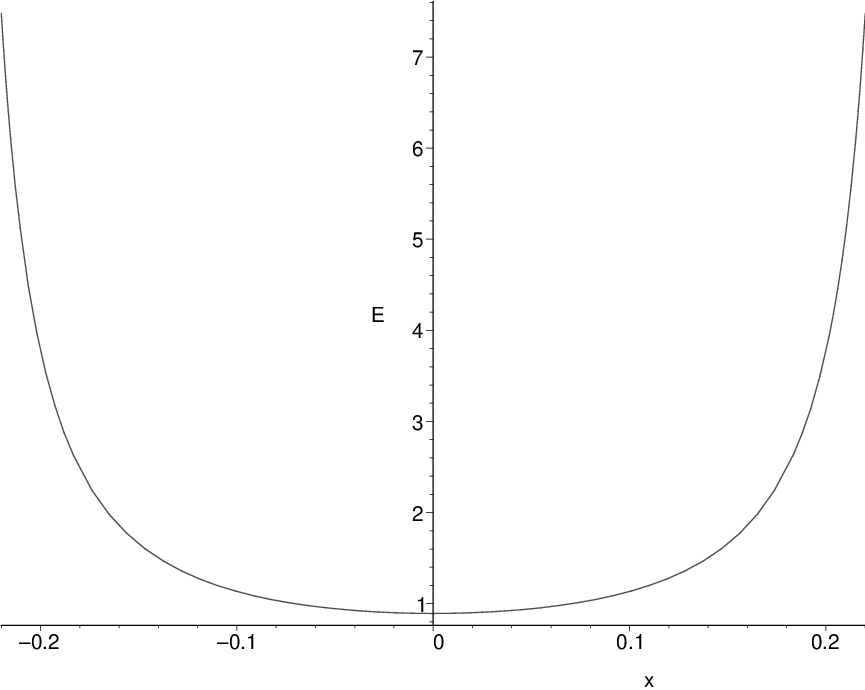
Example 1. (Newton’s egg curve) Suppose $\partial\Omega=\{(x,y):y^{2}=(x^{2}-1)(x-3),\;x\in[-1,1]\}$ (see Figure 1). For the data

w(x,y)=-y^{2}+(x^{2}-1)(x-3),

the equation (5) is reduced to the ODE $(3x^{2}-6x-1)E_{0}^{\prime}(x)+(6x-8)E_{0}(x)=-1$ , whose general solution is

E_{0}(x)={C-E_{1}(x)\over{3x^{2}-6x-1}}\exp\left[-{\sqrt{3}\over{3}}\hbox{arctanh}\left({\sqrt{3}\over{2}}(x-1)\right)\right],

for $x\neq 1-2/\sqrt{3}$ , where $E_{1}^{\prime}(x)=\exp\left[\sqrt{3}/3\;\hbox{arctanh}\left((x-1)\sqrt{3}/2\right)\right].$ Figure 2 shows the parameters satisfying the conditions $E(-1)=0.2$ , and, respectively, $E(1)=0.2$ . The parameter $E$ cannot be determined for $x_{0}=1-2/\sqrt{3}$ .

Refer to caption — Figure 1: The boundary $\partial\Omega=\{(x,y):y^{2}-(x^{2}-1)(x-3)=0,\;x\in[-1,1]\}$ and the data $w(x,y)=-y^{2}+(x^{2}-1)(x-3)$ discussed in Example 1.

Example 2. (Granville’s egg curve) Consider $\partial\Omega=\{(x,y):x^{2}y^{2}=(x-3)(1-x),\;x\in[1,3]\}$ (see Figure 3) and the data given by

w(x,y)=-y^{2}+{(x-3)(1-x)\over{x^{2}}}.

The reduced ODE $2x(2x-3)E_{0}^{\prime}(x)+2(x^{4}-4x+9)E_{0}(x)=x^{4}$ implies

E(x,y)=E_{0}(x)={[C+E_{1}(x)]x^{3}\over{(2x-3)^{43/16}}}\exp\left[{x\over{24}}(4x^{2}+9x+27)\right],

which is defined for $x\neq 1.5$ , where $E_{1}^{\prime}(x)=0.5(2x-3)^{27/16}\exp\left[{x\over{24}}(4x^{2}+9x+27)\right]$ . Similarly, as in Example 1, the parameter cannot be determined for $x=1.5$ . See Figure 4 for $E(1)=0.2$ and, respectively, $E(3)=0.6$ .

Example 3. (Generalized Lamé curve) For $\partial\Omega=\{(x,y):x^{4}+y^{2}=1,\;x\in[-1,1]\}$ (see Figure 5) and the following data

w(x,y)=1-x^{4}-y^{2},

the PDE (5) becomes $4x^{3}E_{0}^{\prime}(x)+2(6x^{2}+1)=1$ . It results

E_{0}(x)=\frac{1}{4x^{2}}+\left[\frac{\sqrt{\pi}}{8x^{3}}\hbox{erf}\left(\frac{1}{2x}\right)+\frac{C}{x^{3}}\right]\exp\left(\frac{1}{4x^{2}}\right)

that is defined for $x\neq 0$ (here erf denote is the error function). Therefore, the parameter cannot be estimated at $x=0$ . See Figure 6 for the cases $E_{0}(-1)=0.25$ , and, respectively, $E_{0}(1)=0.25$ .

Example 4. (Rounded corner rectangular domain) Suppose $\partial\Omega=\{(x,y):y^{2}=-8x^{4}+x^{2}+2,x\in[-a,a]\}$ , where $a=\sqrt{1+\sqrt{65}}/4$ (see Figure 7). For the data

w(x,y)=2+x^{2}-8x^{4}-y^{2},

we obtain the following reduced equation $2x(16x^{2}-1)E_{0}^{\prime}(x)+96x^{2}E_{0}(x)=1$ . Thus,

E_{0}(x)={{C_{1}+\sqrt{16x^{2}-1}+\arctan\left(\sqrt{16x^{2}-1}\right)^{-1/2}}\over{2(16x^{2}-1)^{3/2}}}

for $x\in[-a,-0.25)\cup(0.25,a]$ , and

E_{0}(x)={{C_{2}+\sqrt{1-16x^{2}}+\arctan\left(\sqrt{1-16x^{2}}\right)^{-1/2}}\over{2(1-16x^{2})^{3/2}}}

for $x\in(-0.25,0.25)$ . $E$ cannot be determined for $x=\pm 0.25$ . Figure 8 shows the graph of the parameter for $C_{1}=C_{2}=0$ .

5 Conclusion

In this paper we point out another systematic way of finding classes of symmetry reductions related to parameter identification problems of the form (1). Similar to the study in [3], we emphasize that the geometrical significance of the nonlinearity occurring between the data and parameter in (1) can be reflected by the group analysis tool. Seeking different shapes for domains on which the dimension of the problem can be reduced is not an easy task. Therefore, in this paper, we discuss the nonclassical equivalence transformations related to (5). Briefly, to determine these transformations, the data is considered as a dependent variable as well as the parameter, and the nonclassical method (due to Bluman and Cole) is applied to the studied equation. In general, for a known data $w$ , one should check the invariance of this function in (13), where $\xi$ , $\phi$ , and $\psi$ are discussed in §3. Next, from the second equation in (13), the form of the parameter should be obtained in terms of the invariants of the symmetry reduction. At the end, substituting $E$ and $w$ into (5), the dimension of the model should be reduced by one.

Acknowledgements. One of the authors, N. Bîlă would like to thank Prof. Dr. Heinz W. Engl at Johann Radon Institute for Computational and Applied Mathematics (RICAM) who encouraged her to apply the symmetry analysis to parameter identification problems. She is also grateful to Dr. Philipp Kügler at RICAM and Dr. Antonio Leitão at Federal University of Santa Catarina, for many stimulating and rewarding discussions during her stay at RICAM.

References

[1] W. F. Ames, Nonlinear Partial Differential Equations, Academic Press, New York, 1967.
[2] N. Bîlă and J. Niesen, On a new procedure for finding nonclassical symmetries, J. Symbolic Comput., 38, 6(2004), 1523-1533.
[3] N. Bîlă, Application of symmetry analysis to a PDE arising in the car windshield design, SIAM Journal on Applied Mathematics, 65, 1(2004), pp. 113–130.
[4] G. W. Bluman and J. D. Cole, The general similarity solutions of the heat equation, J. Math. Mech., 18 (1969), pp. 1025–1042.
[5] G. W. Bluman and S. Kumei, Symmetries and Differential Equations, Appl. Math. Sci. 81, Springer-Verlag, New York, 1989.
[6] M. S. Bruzóna and M. L. Gandarias, Applying a new algorithm to derive nonclassical symmetries, Commun. in Nonlinear Sci. Numer. Simul., 13, 3(2008), pp. 517–523.
[7] J. Carminati and K. Vu, Symbolic computation and differential equations: Lie symmetries, J. Symbolic Comput., 29 (2000), pp. 95–116.
[8] E. S. Cheb-Terraba and A. D. Roched, Abel ODEs: Equivalence and Integrable Classes, Comput. Phys. Comm., 130, 1(2000), pp. 204–231.
[9] P. A. Clarkson and M. Kruskal, New similarity reductions of the Boussinesq equation, J. Math. Phys., 30 (1989), pp. 2201–2213.
[10] P. A. Clarkson and E. L. Mansfield, Algorithms for the nonclassical method of symmetry reductions, SIAM J. Appl. Math. 54(1994), pp. 1693–1719.
[11] H. W. Engl, M. Hanke, and A. Neubauer, Regularization of Inverse Problems, Kluwer, Dordrecht, The Netherlands, 1996.
[12] K. Eriksson, D. Estep, P. Hansbo, and C. Johnson, Computational Differential Equations, Cambridge University Press, New York, 1996.
[13] G. Gambino, A. M. Greco, and M. C. Lombardo, A group analysis via weak equivalence transformations for a model of tumor encapsulation, J. Phys A: Math. Gen. 37, 12 (2004), pp. 3835–3846.
[14] W. Hereman, Review of symbolic software for the computation of Lie symmetries of differential equations, Euromath Bull., 1 (1994), pp. 45–82.
[15] N. H. Ibragimov, CRC Handbook of Lie Group Analysis of Differential Equations, Vol. 1: Symmetries, Exact Solutions and Conservation Laws, CRC Press, Boca Raton, 1994.
[16] M. Kžížek and L. Liu, Finite element approximation of a nonlinear heat conduction problem in anisotropic media, Comput. Methods Appl. Mech. Engrg., 157 (1998), p. 387-397.
[17] S. Lie, Gesammelte Abhandlungen, Band 4, B. G. Teubner, Leipzig, Germany, 1929, pp. 320–384.
[18] S. V. Meleshko, Generalization of the equivalence transformations, J. Nonlinear Math. Phys., 3, 1-2(1996), pp. 170–174.
[19] P. J. Olver, Applications of Lie Groups to Differential Equations, Grad. Texts in Math. 107, Springer-Verlag, New York, 1986.
[20] L. V. Ovsyannikov, Group Analysis of Differential Equations, W. F. Ames, trans., Academic Press, New York, 1982.
[21] A. D. Polyanin and V. F. Zaitsev, Handbook of Exact Solutions for Ordinary Differential Equations, Chapman & Hall/CRC Press, Boca Raton, Second Edition, 2003.
[22] A. D. Polyanin and V. F. Zaitsev, Handbook of Nonlinear Partial Differential Equations, Chapman & Hall/CRC Press, Boca Raton, 2004.
[23] V. Romano and M. Torrisi, Application of weak equivalence transformations to a group analysis of a drift-diffusion model, J. Phys. A: Math. Gen. 32 (1999), pp. 7953–7963.
[24] M. Torrisi and R. Tracinà, Equivalence transformations and symmetries for a heat conduction model, Int. J. of Non-Linear Mechanics, 33 (1998), pp. 473–487.
[25] D. Zwillinger, Handbook of Differential Equations, Third Edition, Academic Press, Boston, 1997.

Nonclassical equivalence transformations associated with a parameter identification problem Thanks: This work was partially supported by the Austrian Science Foundation FWF, Project SFB 1308 ”Large Scale Inverse Problems”.