NLO QCD corrections to ${\mathrm{p}}{\mathrm{p}}{\to}{\mathrm{t}}\bar{\mathrm{t}}{\mathrm{b}}\bar{\mathrm{b}}{+}X$ via quark–antiquark annihilation Thanks: This work is supported by the European Community’s Marie-Curie Research Training Network under contract MRTN-CT-2006-035505 “Tools and Precision Calculations for Physics Discoveries at Colliders”.

The search for new particles will be the primary task of the LHC. The discovery of new particles first of all requires to establish excess of events over background. The situation at the LHC is particularly complicated by the fact that for many expected signals the corresponding background cannot entirely be determined from data, but has to be assessed upon combining measurements in signal-free regions with theory-driven extrapolations. To this end, a precise prediction for the background is necessary, in particular including NLO corrections in QCD. Since many of these background processes involve three, four, or even more particles in the final state, this kind of background control requires NLO calculations at the technical frontier. This problem lead to the creation of an “experimenters’ wishlist for NLO calculations” at the Les Houches workshop 2005 [1], updated in 2007 [2], which triggered great theoretical progress in recent years (see Ref. [2] and references therein). Meanwhile the listed processes involving at most five particles in loops have been completed in NLO QCD, including the production of ${\mathrm{W}}{\mathrm{W}}+\mathrm{jet}$ [3], weak-boson pairs plus two jets via vector-boson fusion [4], and triple weak-boson production [6, 5]. However, none of the true $2\to 4$ processes has yet been addressed at NLO.¹¹ 1 Progress in the calculation of the virtual corrections to $\mathrm{u}\bar{\mathrm{u}}\to\mathrm{s}\bar{\mathrm{s}}\mathrm{b}\bar{\mathrm{b}}$ was reported in Ref. [7]. Among those processes, ${\mathrm{p}}{\mathrm{p}}\to{\mathrm{t}}\bar{\mathrm{t}}{\mathrm{b}}\bar{\mathrm{b}}+X$ has top priority.

This process represents a very important background to ${\mathrm{t}}\bar{\mathrm{t}}{\mathrm{H}}$ production where the Higgs boson decays into a ${\mathrm{b}}\bar{\mathrm{b}}$ pair. While early studies of ${\mathrm{t}}\bar{\mathrm{t}}{\mathrm{H}}$ production at ATLAS [8] and CMS [9] suggested even discovery potential of this process for a light Higgs boson, more recent analyses [10, 11] with more realistic background assessments show that the signal significance is jeopardized if the background from ${\mathrm{t}}\bar{\mathrm{t}}{\mathrm{b}}\bar{\mathrm{b}}$ and ${\mathrm{t}}\bar{\mathrm{t}}+\mathrm{jets}$ final states is not controlled very well. This is a clear call for improved signal and background studies based on NLO predictions to these complicated processes. For the ${\mathrm{t}}\bar{\mathrm{t}}{\mathrm{H}}$ signal [12] and the ${\mathrm{t}}\bar{\mathrm{t}}+\mathrm{1jet}$ background [13] at the LHC such predictions have been accomplished in recent years.

The dominant mechanism to produce ${\mathrm{t}}\bar{\mathrm{t}}{\mathrm{b}}\bar{\mathrm{b}}$ final states in hadronic collisions is pure QCD. In leading order (LO) quark–antiquark ($q\bar{q})$ and gluon–gluon (${\mathrm{g}}{\mathrm{g}}$) initial states contribute, where the latter strongly dominate at the LHC because of the high gluon flux. Being of order $\alpha^{4}_{\mathrm{s}}$ the corresponding cross sections are affected by a very large scale uncertainty, which amounts to a factor two or more. Technically the $q\bar{q}$ channel is simpler to deal with—though still demanding—and thus represents a natural first step towards a full treatment of ${\mathrm{p}}{\mathrm{p}}\to{\mathrm{t}}\bar{\mathrm{t}}{\mathrm{b}}\bar{\mathrm{b}}+X$ at NLO. In these proceedings we briefly report on this first step, which was accomplished in Ref. [14].

In LO QCD seven different Feynman diagrams (Fig. 1) contribute to the partonic process $q\bar{q}\to{\mathrm{t}}\bar{\mathrm{t}}{\mathrm{b}}\bar{\mathrm{b}}$. The virtual QCD corrections comprise about 200 one-loop diagrams, which include 8 hexagons and 24 pentagons (Fig. 2). The real corrections, $q\bar{q}\to{\mathrm{t}}\bar{\mathrm{t}}{\mathrm{b}}\bar{\mathrm{b}}{\mathrm{g}}$, are described by 64 diagrams, which result from the LO graphs upon adding an external gluon in all possible ways. In the following we briefly describe the calculation of the virtual and real corrections and present numerical results for the LHC. The calculation has been worked out twice and independently, resulting in two completely independent computer codes, which we denote as version 1 and 2.

The general strategy for the evaluation of the one-loop corrections is based on the reduction of the amplitude ${\cal{M}}^{(\Gamma)}$ of each (sub)diagram $\Gamma$ in the following way,

where the colour structure ${\cal C}^{(\Gamma)}$ present in the (sub)diagram is factorized from the remaining colour-independent part. While loop diagrams that involve a quartic gluon vertex give rise to $3$ colour-factorized amplitudes ${\cal{M}}^{(\Gamma)}$, in all other diagrams—which constitute the large majority—the colour structure factorizes completely. This implies that the computation time for individual loop diagrams does not scale with the total number of independent colour structures, which is 6 for $q\bar{q}\to{\mathrm{t}}\bar{\mathrm{t}}{\mathrm{b}}\bar{\mathrm{b}}$.

The colour-free part of ${\cal{M}}^{(\Gamma)}$ is written as a linear combination of so-called standard matrix elements (SMEs) $\hat{\cal{M}}_{m}$, which consist of Dirac chains containing the polarization information. Since the computing time scales with the number of SMEs, it is important to reduce the set of SMEs as much as possible. To this end, we employ an algebraic procedure based on four-dimensional relations that are derived from Chisholm’s identity and are applied after separation of UV and IR singularities. For massless external fermions this four-dimensional reduction has been described in detail in Sections 3.1 and 3.3 of Ref. [15]; here we had to generalize this approach to one massive and two massless spinor chains (b quarks are treated as massless particles). In this way some thousand different spinor chains are reduced to about 150 SMEs $\hat{\cal{M}}_{m}$.

The most time-consuming components of the numerical calculation are the scalar form factors ${\cal F}^{(\Gamma)}_{m}$, which are linear combinations of the Lorentz-invariant coefficients of $N$-point tensor loop integrals with rank $R\leq 3$ and degree $N\leq 6$,

The evaluation of the tensor coefficients $T^{N}_{j_{1},\dots,j_{R}}$ follows the strategy of Refs. [16, 17] that was already successfully used to compute the NLO electroweak corrections to ${\mathrm{e^{+}}}{\mathrm{e^{-}}}\to 4\,$fermions [15, 18]. In this approach the analytic expressions are not reduced to master integrals. In contrast, the tensor integrals are evaluated by means of algorithms that perform a recursive reduction to master integrals in numerical form. This avoids huge analytic expressions and permits to adapt the reduction strategy to the specific numerical problems that appear in different phase-space regions. The scalar master integrals are evaluated using the methods and results of Refs. [19, 20]. UV divergences are regularized dimensionally in both evaluations, but IR divergences are treated in different ways as described below. Tensor and scalar 6-/5-point functions are directly expressed in terms of 5-/4-point integrals [16, 17]. Tensor 4-point and 3-point integrals are reduced to scalar integrals with the Passarino–Veltman algorithm [21] as long as no small Gram determinant appears in the reduction. If small Gram determinants occur, two alternative schemes are applied [17]. One method makes use of expansions of the tensor coefficients about the limit of vanishing Gram determinants and possibly other kinematical determinants. In the second (alternative) method we evaluate a specific tensor coefficient, the integrand of which is logarithmic in Feynman parametrization, by numerical integration. Then the remaining coefficients as well as the standard scalar integral are algebraically derived from this coefficient.

Version 1 of the virtual corrections starts with the generation of Feynman diagrams using FeynArts 1.0 [22]. Their algebraic reduction is completely performed with in-house Mathematica routines. In detail, $D$-dimensional identities (Dirac algebra, Dirac equation) are used until UV divergences cancel against counterterms. The IR (soft and collinear) divergences are regularized dimensionally and expressed in terms of scalar 2- and 3-point integrals as described in Ref. [23], keeping the full dependence on $D$. It turns out that no $D$-dependent prefactors occur in front of the IR-singular $B_{0}$ and $C_{0}$ integrals. In Ref. [14] we show that this result of our specific calculation is not accidental, but generalizes to arbitrary processes at NLO in the Feynman gauge. Having cancelled UV divergences against counterterms and controlled the $D$-dimensional issues concerning IR singularities, the amplitude is further simplified by reducing the SMEs in four space–time dimensions.

Version 2 of the virtual corrections employs FeynArts 3.2 [24] for generating and FormCalc 5.2 [25] for preprocessing the amplitudes. The first part of the calculation is performed in $D$ dimensions. In particular, the so-called rational terms resulting from the UV divergences of tensor loop coefficients are automatically extracted by FormCalc. Since the IR divergences that appear in the $q\bar{q}$ channel are of abelian nature, we exploit the fact that they can be regularized as in QED by means of fermion and gauge-boson (gluon) masses, $m_{q}$ and $m_{\mathrm{g}}$. These masses are treated as infinitesimal quantities (with $m_{\mathrm{g}}\ll m_{q}$) both in the algebraic expressions and in the numerical routines that evaluate the tensor integrals, i.e. only the logarithmic dependence on these mass parameters is retained. Corresponding IR singularities associated with real emission have been obtained from Ref. [26] by means of an appropriate change of regularization scheme.

In both evaluations the singularities from soft or collinear gluon emission are isolated via dipole subtraction [26, 27, 28] for NLO QCD calculations using the formulation [26] for massive quarks. After combining virtual and real corrections, singularities connected to collinear configurations in the final state cancel for collinear-safe observables automatically after applying a jet algorithm. Singularities connected to collinear initial-state splittings are removed via factorization by PDF redefinitions. The phase-space integration is performed with multichannel Monte Carlo generators [29] and adaptive weight optimization similar to the one implemented in RacoonWW [30].

In version 1 of the real corrections the matrix elements have been calculated using the Weyl–van-der-Waerden spinor technique in the formulation of Ref. [31]. Soft and collinear singularities are regularized using dimensional regularization. The phase-space integration, implemented in C++, is based on RacoonWW, but the phase-space mappings are build up in a more generic way very similar to the approach of Lusifer [32].

In version 2 of the real corrections the matrix elements have been generated with Madgraph [33]. As in the virtual corrections, soft singularities are regularized by an infinitesimal gluon mass and collinear singularities by small quark masses, which appear only in logarithms in the endpoint part of the subtraction function. The Monte Carlo generator is a further development of the one used in COFFER$\gamma\gamma$ [34] and for the calculation of the NLO corrections to ${\mathrm{p}}{\mathrm{p}}\to\mathrm{jj}{\mathrm{H}}+X$ [35]. For the purpose of checking, we have also implemented two-cut-off slicing. In this approach the singular parts of the phase-space integration, which originate from the soft region $E_{\mathrm{g}}<\delta_{\mathrm{s}}\sqrt{\hat{s}}/2$ and the collinear regions $1-\cos(\theta_{{\mathrm{g}}q})<\delta_{\mathrm{c}}$, are treated by means of the well-known soft/collinear approximations. When adding all contributions, the ${\cal O}(\delta_{\mathrm{s,c}})$ dependence on the technical cuts cancels if the cut-off parameters are chosen small enough.

We present predictions for ${\mathrm{p}}{\mathrm{p}}\to{\mathrm{t}}\bar{\mathrm{t}}{\mathrm{b}}\bar{\mathrm{b}}+X$ at $\sqrt{s}=14\,\mathrm{TeV}$. For the top-quark mass we take $m_{\mathrm{t}}=172.6\,\mathrm{GeV}$, while all other QCD partons (including ${\mathrm{b}}$ quarks) are treated as massless. Final states involving collinear gluons and b-quarks are recombined into collinear-safe jets by means of the $k_{\mathrm{T}}$-algorithm of Ref. [36]. Specifically we require two b-quark jets with separation $\sqrt{\Delta\phi^{2}+\Delta y^{2}}>D=0.8$ in the rapidity–azimuthal-angle plane. This sets an effective lower limit on the invariant mass $m_{{\mathrm{b}}\bar{\mathrm{b}}}$ of the b-quark pair, thereby avoiding collinear singularities from ${\mathrm{g}}\to{\mathrm{b}}\bar{\mathrm{b}}$ splittings. Motivated by the search for a ${\mathrm{t}}\bar{\mathrm{t}}H(H\to{\mathrm{b}}\bar{\mathrm{b}})$ signal at the LHC [10, 11], we impose the following additional cuts on the transverse momenta, rapidity and invariant mass of the b-quark jets: $p_{{\mathrm{T}},{\mathrm{b}}}>20\,\mathrm{GeV}$, $|y_{\mathrm{b}}|<2.5$ and $m_{{\mathrm{b}}\bar{\mathrm{b}}}>m_{{\mathrm{b}}\bar{\mathrm{b}},\mathrm{cut}}$. We use CTEQ6 PDFs [37] with $\Lambda_{5}^{\mathrm{LO}}=165\,\mathrm{MeV}$ at LO and $\Lambda_{5}^{\overline{\mathrm{MS}}}=226\,\mathrm{MeV}$ at NLO. For the renormalization and factorization scales we use the central value $\mu_{0}=m_{\mathrm{t}}+m_{{\mathrm{b}}\bar{\mathrm{b}},\mathrm{cut}}/2$ and, to estimate the scale uncertainty, we vary these scales in the range $\mu_{0}/2<\mu<2\mu_{0}$ in a uniform and antipodal way, i.e. with $\mu_{\mathrm{R}}=\mu_{\mathrm{F}}=\mu$ and $\mu_{\mathrm{R}}=\mu_{0}^{2}/\mu_{\mathrm{F}}=\mu$.

Figure 3 shows the total LO cross section and the contribution induced by $q\bar{q}$ annihilation as a function of $m_{{\mathrm{b}}\bar{\mathrm{b}},\mathrm{cut}}$. The ${\mathrm{g}}{\mathrm{g}}$ channel dominates over $q\bar{q}$ annihilation by roughly a factor of 17. The scale uncertainty, displayed by the bands, amounts to a factor 1.6 and is dominated by the $\mu_{\mathrm{R}}$-dependence owing to the large power of $\alpha_{\mathrm{s}}(\mu_{\mathrm{R}})^{4}$ in the LO cross section. Figure 4 illustrates the mutual agreement between NLO results for the $q\bar{q}$ channel obtained with dipole subtraction and phase-space slicing. Here we set $m_{{\mathrm{b}}\bar{\mathrm{b}},\mathrm{cut}}=0$, i.e. $\mu_{0}=m_{\mathrm{t}}$. We observe that, within integration errors, the slicing results become independent of the soft cut-off $\delta_{\mathrm{s}}$ for $\delta_{\mathrm{s}}\mathrel{\raisebox{-3.00003pt}{$\stackrel{{\scriptstyle\displaystyle<}}{{\sim}}$}}10^{-3}$ and agree with the result in the subtraction method. For the $\delta_{\mathrm{c}}$-dependence we find a similar behaviour [14]. Figure 5 shows the reduction of the scale dependence of the $q\bar{q}$ contribution upon going from LO to NLO.

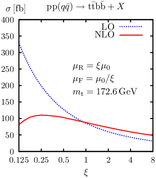
Setting $m_{{\mathrm{b}}\bar{\mathrm{b}},\mathrm{cut}}=0$, at $\mu=\mu_{0}=m_{\mathrm{t}}$ we find $\sigma_{\mathrm{LO}}=85.522(26)\,\mathrm{fb}$ and $\sigma_{\mathrm{NLO}}=87.698(56)\,\mathrm{fb}$, and we observe that (uniform and antipodal) scale variations in the range $\mu_{0}/2<\mu<2\mu_{0}$ shift the cross section by 55% in LO and by 17% in NLO. Figure 6 displays the dependence of the LO and NLO cross sections on the invariant-mass cut $m_{{\mathrm{b}}\bar{\mathrm{b}},\mathrm{cut}}$. The central scale and the uncertainty bands are as in Figure 3.

The reduction of the scale uncertainty from about $\pm 50\%$ to $\pm 17\%$ holds true for the considered range in $m_{{\mathrm{b}}\bar{\mathrm{b}},\mathrm{cut}}$. While the NLO prediction is consistent with the LO uncertainty band, the shape of the distribution is distorted by the corrections. For the central scale, $\mu_{0}=m_{\mathrm{t}}+m_{{\mathrm{b}}\bar{\mathrm{b}},\mathrm{cut}}/2$, we find an NLO correction of $+2.5\%$ for small $m_{{\mathrm{b}}\bar{\mathrm{b}},\mathrm{cut}}$ but a correction of $-10.6\%$ for $m_{{\mathrm{b}}\bar{\mathrm{b}},\mathrm{cut}}=200\,\mathrm{GeV}$.

In order to validate the numerical stability of the tensor reduction we compared the results of the two independent codes finding very good agreement both for single phase-space points and integrated quantities. The CPU time needed to evaluate the virtual corrections for a phase-space point (including sums over colours and polarizations) amounts to about 10 ms on a 3 GHz Intel Xeon processor. This demonstrate that the employed diagrammatic techniques permit a fast and numerically stable evaluation of six-particle processes at the LHC. Based on these encouraging results, we expect to be able to extend this calculation to the technically more challenging gluon-fusion channel.

References

- [1] C. Buttar et al. [QCD, EW, and Higgs Working Group], hep-ph/0604120.
- [2] Z. Bern et al. [NLO Multileg Working Group], arXiv:0803.0494 [hep-ph].
- [3] S. Dittmaier, S. Kallweit and P. Uwer, Phys. Rev. Lett. 100 (2008) 062003 [arXiv:0710.1577 [hep-ph]]; J. M. Campbell, R. K. Ellis and G. Zanderighi, JHEP 0712 (2007) 056 [arXiv:0710.1832 [hep-ph]]; S. Karg and G. Sanguinetti, arXiv:0806.1394 [hep-ph].
- [4] B. Jäger, C. Oleari and D. Zeppenfeld, JHEP 0607 (2006) 015 [hep-ph/0603177]; Phys. Rev. D 73 (2006) 113006 [hep-ph/0604200]; G. Bozzi et al., Phys. Rev. D 75 (2007) 073004 [hep-ph/0701105].
- [5] V. Hankele and D. Zeppenfeld, Phys. Lett. B 661 (2008) 103 [arXiv:0712.3544 [hep-ph]]; T. Binoth et al., arXiv:0804.0350 [hep-ph].
- [6] A. Lazopoulos, K. Melnikov and F. Petriello, Phys. Rev. D 76 (2007) 014001 [hep-ph/0703273].
- [7] T. Binoth et al., arXiv:0807.0605 [hep-ph].
- [8] ATLAS Collaboration, Technical Design Report, Vol. 2, CERN–LHCC–99–15.
- [9] V. Drollinger, T. Müller and D. Denegri, hep-ph/0111312.
- [10] J. Cammin and M. Schumacher, ATL-PHYS-2003-024.
- [11] S. Cucciarelli et al., CMS Note 2006/119; D. Benedetti et al., J. Phys. G 34 (2007) N221.
- [12] W. Beenakker et al., Phys. Rev. Lett. 87 (2001) 201805 [hep-ph/0107081]; Nucl. Phys. B 653 (2003) 151 [hep-ph/0211352]; S. Dawson et al., Phys. Rev. D 67 (2003) 071503 [hep-ph/0211438]; Phys. Rev. D 68 (2003) 034022 [hep-ph/0305087].
- [13] S. Dittmaier, P. Uwer and S. Weinzierl, Phys. Rev. Lett. 98 (2007) 262002 [hep-ph/0703120].
- [14] A. Bredenstein, A. Denner, S. Dittmaier and S. Pozzorini, arXiv:0807.1248 [hep-ph].
- [15] A. Denner et al., Nucl. Phys. B 724 (2005) 247 [hep-ph/0505042].
- [16] A. Denner and S. Dittmaier, Nucl. Phys. B 658 (2003) 175 [hep-ph/0212259].
- [17] A. Denner and S. Dittmaier, Nucl. Phys. B 734 (2006) 62 [hep-ph/0509141].
- [18] A. Denner et al., Phys. Lett. B 612, 223 (2005) [hep-ph/0502063].
- [19] G. ’t Hooft and M. Veltman, Nucl. Phys. B 153 (1979) 365.
- [20] W. Beenakker and A. Denner, Nucl. Phys. B 338 (1990) 349; A. Denner, U. Nierste and R. Scharf, Nucl. Phys. B 367 (1991) 637.
- [21] G. Passarino and M. Veltman, Nucl. Phys. B 160 (1979) 151.
- [22] J. Küblbeck, M. Böhm and A. Denner, Comput. Phys. Commun. 60 (1990) 165.
- [23] S. Dittmaier, Nucl. Phys. B 675 (2003) 447 [hep-ph/0308246].
- [24] T. Hahn, Comput. Phys. Commun. 140 (2001) 418 [hep-ph/0012260].
- [25] T. Hahn and M. Perez-Victoria, Comput. Phys. Commun. 118 (1999) 153 [hep-ph/9807565]; T. Hahn, Nucl. Phys. Proc. Suppl. 89 (2000) 231 [hep-ph/0005029].
- [26] S. Catani et al., Nucl. Phys. B 627 (2002) 189 [hep-ph/0201036].
- [27] S. Catani and M. H. Seymour, Nucl. Phys. B 485 (1997) 291 [Erratum-ibid. B 510 (1998) 503] [hep-ph/9605323].
- [28] S. Dittmaier, Nucl. Phys. B 565 (2000) 69 [hep-ph/9904440].
- [29] F. A. Berends, R. Pittau and R. Kleiss, Nucl. Phys. B 424 (1994) 308 [hep-ph/9404313] and Comput. Phys. Commun. 85 (1995) 437 [hep-ph/9409326]; F. A. Berends, P. H. Daverveldt and R. Kleiss, Nucl. Phys. B 253 (1985) 441; J. Hilgart, R. Kleiss and F. Le Diberder, Comput. Phys. Commun. 75 (1993) 191.
- [30] A. Denner et al., Nucl. Phys. B 560 (1999) 33 [hep-ph/9904472] and Comput. Phys. Commun. 153 (2003) 462 [hep-ph/0209330].
- [31] S. Dittmaier, Phys. Rev. D 59 (1999) 016007 [hep-ph/9805445].
- [32] S. Dittmaier and M. Roth, Nucl. Phys. B 642 (2002) 307 [hep-ph/0206070].
- [33] T. Stelzer and W.F. Long, Comput. Phys. Commun. 81 (1994) 357 [hep-ph/9401258].
- [34] A. Bredenstein, S. Dittmaier and M. Roth, Eur. Phys. J. C 44 (2005) 27 [hep-ph/0506005].
- [35] M. Ciccolini, A. Denner and S. Dittmaier, Phys. Rev. Lett. 99 (2007) 161803 [arXiv:0707.0381 [hep-ph]]; Phys. Rev. D 77 (2008) 013002 [arXiv:0710.4749 [hep-ph]].
- [36] G. C. Blazey et al., hep-ex/0005012, in Proceedings of the Physics at RUN II: QCD and Weak Boson Physics Workshop, Batavia, Illinois, 4-6 Nov 1999, p. 47.
- [37] J. Pumplin et al., JHEP 0207 (2002) 012 [hep-ph/0201195]; D. Stump et al., JHEP 0310 (2003) 046 [hep-ph/0303013].