Living in a Void: Testing the Copernican Principle with Distant Supernovae
Abstract
A fundamental presupposition of modern cosmology is the Copernican Principle; that we are not in a central, or otherwise special region of the Universe. Studies of Type Ia supernovae, together with the Copernican Principle, have led to the inference that the Universe is accelerating in its expansion. The usual explanation for this is that there must exist a ‘Dark Energy’, to drive the acceleration. Alternatively, it could be the case that the Copernican Principle is invalid, and that the data has been interpreted within an inappropriate theoretical frame-work. If we were to live in a special place in the Universe, near the centre of a void where the local matter density is low, then the supernovae observations could be accounted for without the addition of dark energy. We show that the local redshift dependence of the luminosity distance can be used as a clear discriminant between these two paradigms. Future surveys of Type Ia supernovae that focus on a redshift range of will be ideally suited to test this hypothesis, and hence to observationally determine the validity of the Copernican Principle on new scales, as well as probing the degree to which dark energy must be considered a necessary ingredient in the Universe.
The concordance model of the Universe combines two fundamental assumptions. The first is that space-time is dynamical, obeying Einstein’s Equations. The second is the ‘Cosmological Principle’, that the Universe is then homogeneous and isotropic on large scales – a generalisation of the Copernican Principle that “the Earth is not in a central, specially favored position” [1]. As a result of these two assumptions we can use the Freidmann-Robertson-Walker (FRW) metric to describe the geometry of the Universe in terms of a single function, the scale factor , which obeys
| (1) |
where is the Hubble rate, is the energy density, is the (constant) curvature of space, and overdots denote time derivatives. The scale factor can then be determined by observing the ‘luminosity distance’ of astrophysical objects. At small this is given by
| (2) |
where is the deceleration rate, and subscript denotes the value of a quantity today. Recent measurements of (, ) using high redshift, Type Ia Supernovae (SNe) have indicated that , i.e. the Universe is accelerating in its expansion [2, 3]. Accelerating expansion is possible in an FRW universe if a fraction of is in the form of a smoothly distributed and gravitationally repulsive exotic substance, often referred to as Dark Energy [4]. The existence of such an unusual substance is unexpected, and requires previously unimagined amounts of fine-tuning in order to reproduce the observations. Nonetheless, dark energy has been incorporated into the standard cosmological model, known as CDM.

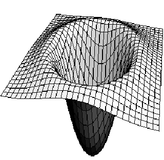

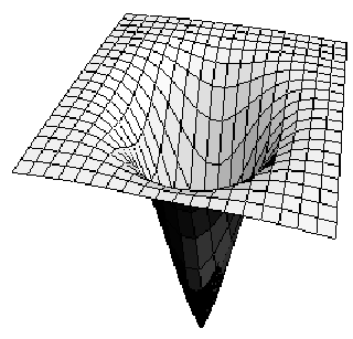
An alternative to admitting the existence of dark energy is to review the postulates that necessitate its introduction. In particular, it has been proposed that the SNe observations could be accounted for without dark energy if our local environment were emptier than the surrounding Universe, i.e. if we were to live in a void [5, 6, 7]. This explanation for the apparent acceleration does not invoke any exotic substances, extra dimensions, or modifications to gravity – but it does require a rejection of the Copernican Principle. We would be required to live near the centre of a spherically symmetric under-density, on a scale of the same order of magnitude as the observable Universe. Such a situation would have profound consequences for the interpretation of all cosmological observations, and would ultimately mean that we could not infer the properties of the Universe at large from what we observe locally.
Within the standard inflationary cosmological model the probability of large, deep voids occurring is extremely small. However, it can be argued that the centre of a large underdensity is the most likely place for observers to find themselves [8]. In this case, finding ourselves in the centre of a giant void would violate the Copernican principle, that we are not in a special place, but it may not violate the Principle of Mediocrity, that we are a ‘typical’ set of observers. Regardless of what we consider the a priori likelihood of such structures to be, we find that it should be possible for observers at their centre to be able to observationally distinguish themselves from their counterparts in FRW universes. Living in a void leads to a distinctive observational signature that, while broadly similar to CDM, differs qualitatively in its details. This gives us a simple test of a fundamental principle of modern cosmology, as well as allowing us to subject a possible explanation for the observed acceleration to experimental scrutiny.
Some efforts have gone into identifying the observational signatures that could result from living in a void. The cosmic microwave background (CMB) supplies us with the tight constraint that we must be within Mpc of the center of the void [9]. There have also been some attempts at calculating predictions for CMB anisotropies and large scale-structure [10, 11, 12], as well as the kinematic Sunyaev-Zeldovich effect [13].
General Relativity allows a simple description of time-dependent, spherical symmetric universes: the Lemaître-Tolman-Bondi (LTB) models [14, 15, 16], whose line-element is
| (3) |
where , and primes denote derivatives . The old FRW scale factor, , has now been replaced by two new scale factors, and , describing expansion in the directions tangential and normal to the surfaces of spherical symmetry. These new scale factors are functions of time, , and distance, , from the centre of symmetry, and obey a generalization of the usual Friedman equation, (1), such that
| (4) |
Here , and is related to the physical energy density by . The two free functions, and , correspond to the curvature of space, and the distribution of gravitating mass in that space. We choose initial conditions such that the curvature is asymptotically flat with a negative perturbation near the origin, and so that the gravitational mass is evenly distributed. As the space-time evolves the energy density in the vicinity of the curvature perturbation is then dispersed, and a void forms. Observations of distant astro-physical objects in this space-time obey a distance-redshift relation
| (5) |
where
| (6) |
and subscript denotes the value of a quantity at the moment the observed photon was emitted. This expression is modified from equation (2), allowing for the possibility of apparent acceleration without dark energy.
We find that the form of the void’s curvature profile is of great importance for the observations made by astronomers at its centre. In Figure 1 we plot some simple curvature profiles, together with the corresponding distance moduli as functions of redshift (distance modulus, dm, is defined as the observable magnitude of an astrophysical object, minus the magnitude such an object would have at the same redshift in an empty, homogeneous Milne universe). It is clear from Figure 1 that for the void models there is a strong correlation between and dm; at low redshifts dm traces the shape of . Hence, for a generic, smooth void starts off with near zero slope, where it is locally very similar to a Milne universe, it then increases at intermediate , and later drops off like an Einstein-de Sitter universe. For CDM, we have at low , i.e. a non-zero slope. Thus, although one can always find a void profile that will mimic CDM [17], such a void will have a curvature profile that is strongly cusped, and non-differentiable, at [18] (see the dotted line in Figure 1 or [19]). Conversely, any generalized dark energy model capable of producing a flat at low would be required to change the equation of state extremely rapidly between and . We therefore have a definitive way to distinguish between a realistic smooth void model, and CDM.

We will now compare the smooth void model to the first-year SNe Legacy Survey (SNLS) data, consisting of 115 SNe [20] calibrated with the SALT light-curve fitter[21], and contrast it with CDM. We use the Bayesian information criterion as a figure of merit (see e.g. [22, 23]), and assume one model to be decisively favored over the other if
| (7) |
where is the evidence for a model, is the maximum likelihood of a model, given a data set, is the number of parameters in the model, and is the number of data points. This criterion corresponds to one model being 150 times more likely than the other. The minimal void model under consideration has 6 parameters: 2 to parametrize a Gaussian , and 4 ‘nuisance’ parameters required to calibrate the SNe data. These are absolute magnitude, intrinsic error, and the colour and stretch parameters used in light curve fitting, . Assuming spatial flatness, CDM requires 5 parameters: 1 specifying the fraction of dark energy, and the same 4 nuisance parameters. In a more comprehensive study it may be preferable to perform a full Bayesian evidence analysis, with suitable priors [23]. In the interests of brevity, and to avoid a lengthy discussion of prior probabilities, we have refrained from this for now.
In Figure 2 we show the SNLS data with the two best fit models. Both have similar goodness of fit, but one can discern a qualitative difference between them, which will be distinguishable with future surveys. The best fitting void is underdense at its centre, and has a scale corresponding to Mpc today. This is of the order expected to produce a feature in dm on a scale of , and large enough to avoid strong constraints from galaxy surveys that extend to . On the other hand, the best fitting CDM model contains dark energy, and fits the data slightly better with . Thus, while the current data marginally prefers CDM, it is not yet able to distinguish between the two models decisively.
One will, of course, be interested in results from other SNe compilations. Using the Riess gold data [24], with the MLCS2k2 light-curve fitter, we find our basic results do not change significantly, with a CDM model still being marginally preferred. Thus our analysis does not appear to be substantially effected by the apparent systematic error that led to the identification of the ‘Hubble Bubble’ anomaly [25]. The ‘Union’ data of [26] is the largest compilation of SNe fitted for with the more conservative SALT fitter, and for these 315 SNe (including the ‘outliers’) we find the void model is marginally preferred over CDM, with in favor of a void. It therefore appears neccessary to obtain more data, in order to be able to decisively distinguish the two models.

Due to the different strategies and technologies, SNe surveys typically target either low or high redshifts. This has lead to a dearth of SNe at – exactly the location where there is the greatest qualitative difference between the two models. Future SNe surveys, with a redshift coverage in this region, will do better. As an example of the future constraints we can expect to gain, we consider the JDEM missions which expect to observe 2000 high redshift SNe in the interval , with an expected smooth distribution [27]. At very low redshifts () a further 300 SNe can be expected to be observed by other projects. We consider data simulated from a CDM model, using the SALT fitter, and a Gaussian void model with the same parameter values as before. In both cases we find that these 2300 SNe are sufficient to decisively recover the correct underlying model. For the void model we find , while for the CDM model . These are considerably better than the decisive benchmark, which was satisfied by all 1000 of our simulations (except one in the CDM case). We can therefore say with confidence that the upcoming SNe data will be able to distinguish CDM from a void model, independent of which is responsible for the apparent acceleration.
Given that 2300 SNe from a JDEM mission will do a superfluous job, we will now estimate the minimum number of SNe required to meet the bound in Equation (7). Using the same redshift distribution as before [27], we now consider different numbers of SNe. In the case of the void cosmology we find that with 170 SNe 50% of our 1000 simulations recovered the void model decisively, while with 480 SNe 99% of the simulations could do so. Similarly, in the case of a CDM cosmology we found that with 180 and 700 SNe we could decisively recover the correct model in 50% and 99% of the simulations, respectively. This is illustrated in Fig. 3. These projections are much lower than the number of SNe expected to be observed by the next generation of SNe surveys, and we should therefore expect less ambitious projects to able to distinguish between the two models. In fact, this may be possible soon, with data from the Sloan Survey and third year SNLS expected to be released imminently. The results obtained here depend on the details of the future surveys. Tailoring these to the specific regions where the two models differ most would undoubtedly give decisive results sooner.
Consider now the effect of varying the redshift distribution, rather than the overall number. Adding a further 300 SNe to the SNLS data, and letting them have a Gaussian redshift distribution with and a mean that can vary, we simulate the data from void and CDM models. We find that in a void Universe the optimal place to search for these extra 300 SNe is at (limiting ourselves to a mean redshift of less than 1), where the average . In a CDM universe the SNe would be better placed a little lower, at , and in this case .
We emphasise that similar results to those presented above should be obtainable for any smooth void model. For example, repeating our analysis for void (b), in Fig. 1, gives almost identical results to void (a). The reason for this is that all smooth voids display the same qualitative behaviour of having a flat dm() profile at low-. It is this qualitative difference that allows the void models to be so easily distinguished from CDM, and as all smooth voids display this low- behaviour, we expect the results we have presented to be broadly generalizable to all voids. Of course, it may be possible to imagine anomolous cases. This will be considered further in a more extended future publication.
Two very different paradigms have been invoked to explain the current observation of an apparently accelerating Universe, depending on whether we invoke or reject the Copernican Principle. We have shown that in the coming years it will be possible to experimentally distinguish between these two scenarios, allowing us to experimentally test the Copernican Principle [28, 29, 30], as well as determine the extent to which Dark Energy must be considered a neccessary ingredient in the Universe.
Acknowledgements
We are grateful to C. Clarkson, L. Miller, A. Slosar, and M. Sullivan for discussions, and the BIPAC for support. TC acknowledges the support of Jesus College, and KL the Glasstone foundation and Christ Church.
References
- [1] Bondi, H. Cosmology, CUP (Cambridge) (1952).
- [2] Perlmutter, S. et. al. Astrophys. J. 517, 565 (1999).
- [3] Riess, A. et. al., Astron. J. 116, 1009 (1998).
- [4] Albrecht, A. et. al, [astro-ph/0609591].
- [5] Alexander, S., Biswas, T. & Notari, A. [arXiv: 0712.0370].
- [6] Alnes, H., Amarzguioui, M. & Grøn, Ø. Phys. Rev. D73, 083519 (2006).
- [7] Garcia-Bellido, J. & Haugboelle, T. Jour. Cosm. Astropart. Phys. 04, 003 (2008).
- [8] Linde, A. D., Linde, D. A. & Mezhlumian, A. Phys. Lett. B345, 203 (1995).
- [9] Alnes, H. & Amarzguioui, M. Phys. Rev. D74, 103520 (2006).
- [10] Clarkson, C. Phys. Rev. D76, 104034 (2007).
- [11] Zibin, J. P. Phys. Rev. D78, 043504 (2008).
- [12] Hunt, P. & Sarkar, S. [arXiv:0807.4508].
- [13] Garcia-Bellido, J. & Haugboelle, T. [arXiv: 0807.1326].
- [14] Lemaître, G. Ann. Soc. Sci. Brussels A53, 51 (1933).
- [15] Tolman, R. C. Proc. Nat. Acad. Sci. USA 20, 169 (1934).
- [16] Bondi, H. Mon. Not. Roy. Astron. Soc. 107, 410 (1947).
- [17] Mustapha, N., Hellaby, C. & Ellis, G. F. R. Mon. Not. Roy. Astron. Soc. 292, 817 (1997).
- [18] Vanderveld, R. A., Flanagan, E. E. & Wasserman, I. Phys. Rev. D74, 023506 (2006).
- [19] Yoo, C.-M., Kai, T. & Nakao, K.-I. [arXiv:0807.0932].
- [20] Astier, P. et. al. Astron. Astrophys. 447, 31 (2006).
- [21] Guy, J. et. al. Astron. Astrophys. 443, 781 (2005).
- [22] Liddle, A. R. Mon. Not. Roy. Astron. Soc. 377, L74 (2007).
- [23] Liddle, A. R., Mukherjee, P. & Parkinson, D. A & G 47, 4.30 (2006).
- [24] Riess, A. G. et. al. Astrophys. J. 659, 98 (2007).
- [25] Jha, S. et. al. Astrophys. J. 659, 122 (2007).
- [26] Kowalski, M. et. al. [arXiv: 0804.4142].
- [27] Kim, A. G., Linder, E. V., Miquel, R. & Mostek, N. Mon. Not. Roy. Astron. Soc. 347, 909 (2004).
- [28] Uzan, J. P., Clarkson, C. & Ellis, G. F. R. [arXiv: 0801.0068].
- [29] Clarkson, C. et. al. Phys. Rev. Lett. 101, 011301 (2008).
- [30] Caldwell, R. & Stebbins, A. Phys. Rev. Lett. 100, 191302 (2008).