Angle-Resolved Photoelectron Spectroscopy Studies of the Many-Body Effects in the Electronic Structure of High- Cuprates
LEIBNITZ INSTITUT FÜR FESTKÖRPER- UND WERKSTOFFFORSCHUNG
FAKULTÄT MATHEMATIK UND NATURWISSENSCHAFTEN
DER TECHNISCHEN UNIVERSITÄT DRESDEN
Angle-Resolved Photoelectron Spectroscopy Studies of the
Many-Body Effects in the Electronic Structure of High- Cuprates
Dissertation
zur Erlangung des
Doktorgrades der Naturwissenschaften
(Doctor rerum naturalium)
vorgelegt von
Dmytro S. Inosov
geboren am 23. April 1979 in Kiew
© 2005–2008 Dresden
Institute for Solid State Research, IFW Dresden
P. O. Box 270116, D-01171 Dresden, Germany.
Eingereicht am ____ . ____ . 08
Berichterstatter
| 1. Gutachter: | Prof. Dr. Bernd Büchner |
| IFW Dresden | |
| P. O. Box 270116 | |
| D-01171 Dresden | |
| 2. Gutachter: | Prof. Dr. Ilya Eremin |
| Institute für Mathematische und Theoretische Physik | |
| TU-Braunschweig | |
| 38106 Braunschweig | |
| 3. Gutachter: | Dr. Luc Patthey |
| Swiss Light Source, Paul Scherrer Institute | |
| CH-5234 Villigen | |
| Switzerland |
Verteidigt am ____ . ____ . 08
LEIBNITZ INSTITUT FÜR FESTKÖRPER- UND WERKSTOFFFORSCHUNG
FAKULTÄT MATHEMATIK UND NATURWISSENSCHAFTEN
DER TECHNISCHEN UNIVERSITÄT DRESDEN
The undersigned hereby certify that they have read and recommend to the Faculty of Mathematics and Natural Sciences for acceptance a thesis entitled “Angle-Resolved Photoelectron Spectroscopy Studies of the Many-Body Effects in the Electronic Structure of High- Cuprates” by Dmytro S. Inosov in fulfilment of the requirements for the degree of Doctor of Philosophy.
Dated: August 24, 2026
External Examiner:
Prof. Dr. H.-H. Klauß
Research Supervisor:
Prof. Dr. Bernd Büchner
Readers:
Prof. Dr. Ilya Eremin
Dr. Luc Patthey
LEIBNITZ INSTITUT FÜR FESTKÖRPER- UND WERKSTOFFFORSCHUNG
FAKULTÄT MATHEMATIK UND NATURWISSENSCHAFTEN
DER TECHNISCHEN UNIVERSITÄT DRESDEN
Date: August 24, 2026
\@normalsize
- Author:
Dmytro S. Inosov
- Title:
Angle-Resolved Photoelectron Spectroscopy Studies of the Many-Body Effects in the Electronic Structure of High- Cuprates
- Faculty:
Mathematics and Natural Sciences, TU Dresden
- Degree:
Ph.D.
Permission is herewith granted to IFW Dresden and the Faculty of Mathematics and Natural Sciences to circulate and to have copied for non-commercial purposes, at their discretion, the above title upon the request of individuals or institutions.
Signature of AuthorTHE AUTHOR RESERVES OTHER PUBLICATION RIGHTS, AND NEITHER THE THESIS NOR EXTENSIVE EXTRACTS FROM IT MAY BE PRINTED OR OTHERWISE REPRODUCED WITHOUT THE AUTHOR’S WRITTEN PERMISSION.
THE AUTHOR ATTESTS THAT PERMISSION HAS BEEN OBTAINED FOR THE USE OF ANY COPYRIGHTED MATERIAL APPEARING IN THIS THESIS (OTHER THAN BRIEF EXCERPTS REQUIRING ONLY PROPER ACKNOWLEDGEMENT IN SCHOLARLY WRITING) AND THAT ALL SUCH USE IS CLEARLY ACKNOWLEDGED.
Contents
Introduction
Physical reality remains so mysterious even to physicists because of the extreme improbability that it was constructed to be understood by the human mind.
Steven Weinberg
For more than twenty years now the phenomenon of the high-temperature superconductivity [1] has been standing fast against all efforts to find a suitable theory that would describe the behavior of the doped copper oxides in all its diversity. On the one hand, the layered cuprates exhibit a number of anomalous electronic properties in both superconducting and normal states, which seem to slip out of the scope of any conventional theory, therefore making the understanding of these systems unprecedentedly difficult. On the other hand, high-temperature superconductors can be called simple in many respects. First of all, these are layered materials with quasi-two-dimensional electronic structure, which simplifies the treatment of experimental results. Second, some of these materials, like the Bi-based family of cuprates, are easily cleavable and have already become model materials for surface-sensitive experiments, such as photoelectron spectroscopy and tunneling electron microscopy. Third, they become metallic at sufficient doping, which is also essential for the above-mentioned experimental techniques. Such a unique combination of interesting physical properties with experimental accessibility has been stimulating an unceasing interest to the high-temperature superconductors since their discovery in 1986. Since then, the whole branches of condensed matter physics and experimental research have been pushed forward by the endeavor to understand the physics of unconventional superconductors and optimize their critical temperature. Among them is the angle-resolved photoelectron spectroscopy (ARPES), which is the topic of the present work.
In spite of the failures to find an ultimate theory of unconventional superconductivity, after many years of research the scientific community possesses a considerable store of theoretical knowledge about the problem. Over time, the focus is gradually shifted from finding a theoretical description of an experimentally observed phenomenon to distinguishing between multiple models that offer comparably reasonable descriptions. From the point of view of an experimentalist, this means that any qualitative understanding of an experimental observation would no longer suffice. Instead, the emphasis in the experimental research should be shifted to accurate quantification of observations, which becomes possible only if the results available from all the available experimental methods are connected together by the theoretical glue. Among the methods that are to be unified, ARPES plays a central role. The reason for this is that it gives access to the single-particle excitation spectrum of the material as a function of both momentum and energy with very high resolution. Other experimental techniques, such as inelastic neutron scattering (INS), Raman spectroscopy, or the newly established Fourier-transform scanning tunneling spectroscopy (FT-STS) probe more complicated two-particle spectra of the electrons and up to now can not achieve the momentum resolution comparable with that of ARPES. Such reasoning serves as the motivation for the present work, in which some steps are done towards understanding the anomalous effects observed in the single-particle excitation spectra of cuprates and relating the ARPES technique to other experimental methods.
Structure of this thesis. In the first chapter, some aspects of the condensed matter physics and many-body quantum theory are summarized. In particular, the notions of the self-energy, one- and two-particle Green’s functions, and the Bardeen-Cooper-Schrieffer theory of conventional superconductivity are briefly reviewed. The scope of this chapter is kept to the minimum necessary for understanding the main results presented in the subsequent chapters. Where possible, references to the literature containing more extensive information are provided. In spite of conciseness, all attempts were made to keep this chapter in line with the strict theoretical constructions found in modern literature.
The second chapter is an introduction to the angle-resolved photoemission. It consists of two sections covering the theory of photoemission and experimental aspects of ARPES respectively. In the first part, the so-called one- and three-step models of photoemission are discussed in relation to the many-particle systems of increased complexity: non-interacting, interacting, and superconducting. In the experimental part, most attention is paid to the specifics of the experimental setup, experimental geometry, and synchrotron light sources used in the present work. This chapter also contains a description of the sample preparation techniques used.
The third chapter is focused on the electronic properties of Bi2Sr2CaCu2O8+δ — the superconducting cuprate most studied by surface sensitive methods. The chapter starts from the description of its crystal structure and its place among other families of cuprates. Then a report of the recent progress in understanding the electronic structure of this material is presented, focusing mainly on the understanding of the many-body effects (renormalization) and their manifestation in the ARPES spectra. The main result of this chapter is a model of the Green’s function that is later used in chapter 5 for calculating the two-particle excitation spectrum.
The fourth chapter is devoted to the matrix element effects in the photoemission spectra of cuprates. After a general introduction to the problem, is focuses on the recently discovered anomalous behavior of the ARPES spectra that partially originates from the momentum-dependent photoemission matrix element. The momentum- and excitation energy dependence of the anomalous high-energy dispersion, termed “waterfalls”, is covered in full detail. Understanding the role of the matrix element effects in this phenomenon proves crucial, as they obstruct the view of the underlying excitation spectrum that is of indisputable interest.
Finally, the fifth chapter is devoted to the relation of ARPES with other experimental methods, with the special focus on the INS spectroscopy. For the optimally doped bilayer Bi-based cuprate, the renormalized two-particle correlation function in the superconducting state is calculated from ARPES data within an itinerant model based on the random phase approximation (RPA). The results are compared with the experimental INS data on Bi2Sr2CaCu2O8+δ and YBa2Cu3O6.85. The calculation is based on numerical models for the normal and anomalous Green’s functions fitted to the experimental single-particle spectra. The renormalization is taken into account both in the single-particle Green’s function by means of the self-energy, and in the two-particle correlation function by RPA. In the last sections of the same chapter, two other applications of the same approach are briefly sketched: the relation of ARPES to FT-STS, and the nesting properties of Fermi surfaces in two-dimensional charge density wave systems.
Chapter 1 Excerpts From the Many-Body Quantum Theory
1.1 The many-body system
1.1.1 The -particle quantum states
The many-body quantum theory [2, 3, 4, 5, 6, 7, 8, 9] rests upon the simple mathematical fact that if is a basis set in the single-particle state space , then the set of all possible products will be a basis in the -particle state space , i.e. . The single-particle basis set is usually chosen to be the proper basis of the single-particle Hamiltonian, and any many-particle state is represented as a linear combination of the form . This formal expansion is actually the only relationship between a many-particle system and single particles. For convenience, the many-particle basis set is symmetrized (for bosons) or anti-symmetrized (for fermions), being replaced by a set of Slater determinants Here is the group of -element permutations and . In this new basis the coefficients in the expansion of any many-particle state obtain their natural (fermionic or bosonic) symmetry with respect to the permutation of indices. Unfortunately, the possibility to consider the interacting many-particle system as a combination of single particles (as dictated by the reality of the experiment) is achieved here at the expense of the new basis being no longer a proper basis of the many-particle Hamiltonian.
Each element in the -particle basis set is uniquely defined by specifying the indices of the single-particle states that enter the Slater determinant. This allows one to simplify the notation by writing the basis elements in the so-called occupation number representation: , where The complete linear hull of all these basis vectors for all is called the Fock space.
1.1.2 Second quantization
Having the Fock space defined, one can introduce the creation and annihilation operators acting on it. These are denoted as and respectively for bosons and as and for fermions. By definition,
| (1.1a) | ||||
| (1.1b) | ||||
| (1.1c) | ||||
| (1.1d) | ||||
Both pairs of creation and annihilation operators are mutually Hermitian conjugate with the following properties:** * The and operators form a Banach algebra with a norm-preserving involution operator , making it a -algebra [10].
| (1.2a) | |||||||||
| (1.2b) | |||||||||
From now on, for simplicity of notation we will denote by either a boson operator or a fermion operator . In this notation a basis state will be written as .
A special case of the creation operator is the so-called quantum field operator , which creates a delta-function at point .
As a rule, every term entering the Hamiltonian of a physical system is either a local single-particle operator , such as the kinetic energy operator , or a two-particle operator , such as the Coulomb interaction . In second quantization notation, such operators can be rewritten as:†† † The proof is straightforward and can be found in Ref. [2], p. 14.
| (1.3) | ||||
| (1.4) |
The order of indices in the coefficients is chosen in such a way that corresponds to a transition from the initial state to the final state . Explicit expansions of some commonly used operators in second quantization are collected in table 1.1.
| Electromagnetic field: | , |
|---|---|
| where is the polarization vector. | |
| Kinetic energy operator: | |
| Spin operator: | |
| Coulomb interaction: | |
| Charge density operator: | |
| Spin density operator: |
1.1.3 Non-interacting electron gas
The simplest possible generalization of a single-electron problem is the non-interacting electron gas within the so-called jellium model, which means that the external periodic potential is replaced by its average (a constant) and is therefore neglected. The word ‘non-interacting’ here means that no particle-particle interaction terms enter the Hamiltonian:
| (1.5) |
but the electrons still feel each other through Pauli exclusion principle and are therefore not independent. The ground state of such a system is a Fermi sphere: . At zero temperature it consists of plane waves filling all states with , being the energy of the topmost occupied state (Fermi energy). At finite temperatures, the occupation number is given by the Fermi-Dirac distribution , where .
The same problem can be also considered in the periodic potential, with the only difference that the natural basis in this case is a set of Bloch waves. But in case of localized electrons (tightly bound to their parent atom), it is reasonable however to change the basis to localized wave functions that would approach atomic orbitals of individual atoms in the atomic limit [4, p. 194].
Wannier functions [11] centered at lattice sites are defined to be
| (1.6) |
where index enumerates the states within some energy band, and incorporates the rest of quantum numbers, thus enumerating different energy bands. The Wannier functions for all and form an orthonormal basis, and the Bloch functions can be recovered from them by computing
| (1.7) |
As each Bloch function is defined only up to an overall phase factor, the Wannier functions can be rewritten as
| (1.8) |
where is an arbitrary real function.
By manipulating , one can try to optimize the Wannier functions so that they drop off as fast as possible when moves away from . Such localization is possible whenever there is an energy gap separating the band from any other one. When two bands have a point at which they are degenerate, it is not possible to construct localized wave functions out of the Bloch states [4, p. 197]. For an insulator, the localized Wannier functions are approaching the atomic orbitals, which makes it possible in many applications to approximate the Wannier functions by the corresponding atomic orbitals .
Eq. (1.7), restricted to the -th band, can be rewritten in the second quantization as
| (1.9) |
where the operators and create an electron in the states and respectively.
By analogy with (1.5) the system’s Hamiltonian will be
| (1.10) |
where the matrix element is the energy of the state . By substitution of (1.9) it can be rewritten as
| (1.11) |
If the Wannier functions are localized around their parent atoms, the sum (1.11) can be restricted to several nearest neighbors only, which is called the tight binding approximation:
| (1.12) |
where indicates a sum over distinct nearest neighbor pairs, and are the so-called tight binding parameters that characterize the overlap of the Wannier functions on different sites and are often called hopping integrals.‡‡ ‡ According to the physical folklore, the electron “hops” from site to site . This notion is somewhat misleading, because “hopping” suggests that there is some time-dependence in the electron’s behavior which contradicts the fact that we are dealing with a time-independent Schrödinger equation.
1.1.4 Interacting electron gas
The general form of the Hamiltonian for the interacting electron gas in the tight binding model is
| (1.13) |
The first (bilinear) term includes the kinetic energy operator and interaction with the external potential, while the second term represents the electron-electron interaction. The prime over the summation sign indicates that no equal electronic states should appear in the creation and annihilation parts of each summation term (in order to exclude the bilinear terms already included in the first sum).
A simplification to this Hamiltonian was proposed by Hubbard in 1963 [12] to study the electronic correlations leading to magnetism and was solved exactly in one dimension by Lieb and Wu in 1968 [13]. In the so-called Hubbard model, only several nearest-neighbor bilinear terms are usually considered and the Coulomb interaction between electrons on different sites is neglected:
| (1.14) |
Here is the so-called on-site repulsion (energy lost if two electrons with opposite spins occupy the same orbital), also known as Hubbard , and is the occupation number of the state . Thus, the Hubbard model is the simplest possible extension of the tight-binding model that introduces an energy penalty for any atomic site occupied by more than one electron. The two limiting cases of the Hubbard model are (nearest neighbor tight-binding model) and (atomic limit).
If one considers the Hubbard model with a single (most significant) hopping term and treats this term as a perturbation (assuming ) [14], in the second order of the perturbation theory the Hamiltonian will take the form, which is referred to as the - model:
| (1.15) |
where is the effective interatomic exchange interaction constant.
In the particular case of half-filling, the - Hamiltonian does no longer explicitly contain , and only the exchange interaction term is preserved:
| (1.16) |
This Hamiltonian was first considered by Heisenberg [15] and describes the so-called localized electron model, appropriate for the description of magnetic insulators. We will return to the discussion of this model in §5.2.1, where it will be compared with the alternative itinerant electron model.
1.2 The concept of the Green’s function
1.2.1 Single-particle Green’s function
Consider the following Schrödinger equation, where is a perturbation:
| (1.17) |
By definition, the unperturbed Green’s operator (or Green’s function) of this equation is
| (1.18) |
The solution to the Schrödinger equation then satisfies the following relationship:
| (1.19) |
This allows solving the Eq. (1.17) iteratively, given that the following limit exists:
| (1.20) |
One can also introduce the Green’s operator for the perturbed Hamiltonian:
| (1.21) |
By analogy with Eq. (1.19), the two Green’s operators can be related via the so-called Dyson equation:
| (1.22) |
It is instructive to rewrite the same equation in Feynman diagrams:
| (1.23) |
Here ††feynman-diagram: (Feynman diagram, (x6) , ††feynman-diagram: (Feynman diagram, (x6) , and ††feynman-diagram: (Feynman diagram, (x1) denote , , and the perturbation respectively. Such notation is meant to visualize the analogy between this simple single-particle equation and the self-energy expansion of the single-particle Green’s function of a many-body system that will be discussed below.
1.2.2 Single-particle Green’s function of a many-body electron system
In a many-body system, the single-particle Green’s functions no longer carry the full information about the system’s wave function. Nevertheless, they are still extremely useful for treating the results of experiments, which are to a large degree defined by one- and two-particle processes.
There are several types of single-particle Green’s functions [2, 3]:
| greater: | (1.24a) | |||||
| lesser: | (1.24b) | |||||
| retarded: | (1.24c) | |||||
| advanced: | (1.24d) | |||||
| time-ordered: | (1.24e) | |||||
| anti-time-ordered: | (1.24f) | |||||
As directly follows from this definition, the retarded and advanced Green’s functions can be also expressed in terms of the greater and lesser Green’s functions:
| (1.25) |
Here the definitions were given in real space representation, but they can also be rewritten in any -basis:
| (1.26) |
For translation-invariant systems, such as an infinite or semi-infinite crystal, which are of interest in the current work, the -representation is the most natural one. In this case becomes due to translation invariance, and in the -representation , i.e. the Green’s function depends on a single argument:
| (1.27) |
As an example, let us consider the greater Green’s function of the non-interacting electron system described by the quadratic Hamiltonian
| (1.28) |
for which the operators have a simple time dependence: and (the so-called bare Green’s function). Because the Hamiltonian is diagonal in , so is the Green’s function:
| (1.29a) | ||||
| Similarly, | ||||
| (1.29b) | ||||
| (1.29c) | ||||
By applying Fourier transform to (1.29a) or (1.29b), one can immediately see that in the frequency domain the greater and lesser Green’s functions of a non-interacting system are localized along the dispersion :
| (1.30a) | ||||
| (1.30b) | ||||
| For the retarded Green’s function the situation is a bit different. Here because of the function the Fourier transform will result in | ||||
| (1.30c) | ||||
Hence, is an analytical function of except for one pole at . The corresponding bare spectral function , which will be important for treating the results of photoemission experiments (see section 2.1), is still localized at .
1.2.3 Renormalization and the concept of self-energy.
In §1.2.1 it was shown how the Green’s operator of a perturbed Hamiltonian can be expressed in terms of the “bare” Green’s operator via the Dyson equation. This was demonstrated in the simplest case of a single-particle Hamiltonian. A similar result holds for the retarded Green’s function (1.27) of a many-body system with small interactions that can be considered as a perturbation. In Feynman notation [16], the perturbation series for the Green’s function§§ § The Feynman notation is usually used only for the time-ordered Matsubara Green’s functions, which will be introduced in §1.2.5, but as long as we do not explicitly write the Feynman rules here, we can formally denote the perturbation expansion for any real-time Green’s function by the same diagrams. is [[6], p. 227; [8], p. 138]
| (1.31) |
The series (1.31) contains repeating patterns of diagrams that allow simplification by denoting
| (1.32) |
The sum (1.32) is called the self-energy and includes all irreducible diagrams (i.e. those that cannot be disconnected by cutting an internal fermion line). Substitution of (1.32) into (1.31) yields the Dyson equation of the form (1.23). Thus the self-energy function is the measure of the perturbation introduced to the bare Hamiltonian by the interaction terms. In Fourier space the Dyson equation turns into a simple algebraic form with the self-energy being a complex-valued function of :
| (1.33) |
The same equation holds also for the advanced Green’s functions, the retarded and advanced self-energies being complex conjugate to each other: . From now on we will work mainly with the retarded Green’s function and self-energy, omitting the upper index R.
Dyson’s equation (1.33) can be rewritten in a slightly different but equivalent form by using the algebraic form for (1.30c):
| (1.34) |
Here we see that the perturbation of the quadratic Hamiltonian causes a shift of the electron dispersion by (so-called renormalization of the bare band) and Lorentzian broadening of the spectral function caused by . This broadening can be interpreted as finite “lifetime” of the single-particle states that are destroyed by the interactions, and the imaginary part of the self-energy is therefore termed scattering rate. It is remarkable that all kinds of interactions (such as electron-electron, electron-phonon, electron-magnon, impurity scattering, etc.) enter as additive terms into the self-energy, making it a universal tool for describing weakly interacting many-particle systems.¶¶ ¶ In spite of these seemingly simple basic ideas, the renormalization group theory is a complicated branch of quantum field theory and mathematics, still being actively explored. The self-energy is represented as a sum of infinitely many Feynman diagrams, which is impossible to calculate exactly. Thus, limiting the sums like (1.32) only to the most significant terms and formalization of the summation procedure utilizing the self-similarities (scaling properties) of the series are the main challenges. For a detailed introduction into the field, see Ref. [2, 3, 17, 7, 6, 9].
Due to the analytical properties of the self-energy, its real and imaginary parts are bound by the following Kramers-Kronig relations:
| (1.35a) | |||
| (1.35b) |
These important relations are discussed in detail in appendix A.
1.2.4 The spectral function
In the previous paragraph the spectral function of an interacting electron gas has been introduced. Here we will derive the expression for the spectral function at finite temperature in Lehmann representation that will be useful later in section 2.1.
We start with the definition of the retarded Green’s function (1.24c) rewritten in the one-particle basis (note that we retain the off-diagonal elements ):
| (1.36) |
Inserting the identity matrix and writing down explicitly the time evolution of the -operators, we obtain the so-called Lehmann representation of the retarded Green’s function [2, p. 128]:
| (1.37) |
which after taking the Fourier transform becomes
| (1.38) |
If we define the spectral function as ∥∥ ∥ In some sources [2, 3], the spectral function is normalized to , rather than to unity, i.e. is defined as . and use the Dirac identity , we have
| (1.39) |
In many applications, the spectral function is considered diagonal, and we will also neglect the off-diagonal components () when treating the photoelectron spectroscopy experiments (§2.1.3).
1.2.5 Imaginary time Green’s functions
The definition of the Green’s functions (1.24) includes thermodynamic averaging, which at a finite temperature can be explicitly written as
| (1.40) |
Because of the similarity between the two exponents and , it appears convenient to extend the time to complex values and consider a special case, when is purely imaginary, so that is real.
The single-particle Matsubara Green’s function, or imaginary-time Green’s function, is defined as
| (1.41) |
where is the imaginary time ordering operator:
| (1.42) |
One can show that the convergence of (1.41) is guaranteed only for . Moreover, the function depends on time difference only, i.e. , and has the symmetry property for . With these properties taken into account, it can be expanded into a Fourier series in the interval :
| (1.43) |
where for bosons and for fermions are the so-called Matsubara frequencies.
By using the Lehmann representation, it is possible to show that the newly introduced function and the retarded Green’s function have a common analytical continuation.**** ** The proof can be found in Ref. [2], p. 189. In other words, there exists a function , , analytic in the upper half-plane, which coincides with on the real axis and with on the imaginary axis. This means that as soon as one of the functions is known analytically, the other one can be immediately obtained by a formal change of variables: . Nevertheless, if only the numerical representation of one of the functions is known, computing the other one by analytical continuation requires an extra level of integration. In most cases, when dealing with perturbation series, the calculations involving Matsubara functions are easier and lead to more compact expressions, which finally need to be continued analytically to the real axis to make any comparison with experimental data possible.
When the Matsubara functions are considered as functions of momentum and frequency , it is convenient to treat both arguments as components of a single 4-dimensional argument, called 4-momentum, with one imaginary and three real components. In this sense, the frequency and momentum components within the same 4-momentum can be denoted by the same letter, e.g. , which makes it easier to distinguish the corresponding arguments in formulae containing more than one 4-momentum.†††† †† Note that the summation indices like are used as single symbols instead of . This allows distinguishing different Matsubara frequency arguments, which would otherwise require using multiple subindices Integration over all 4-momentum arguments is denoted as .
1.3 Two-particle correlation functions
1.3.1 Lindhard function
The single-particle Green’s functions describe the properties of individual particles, renormalized by excitations of the weakly interacting many-body system, within the linear response regime. Still, many experiments, such as resistivity measurements, inelastic light scattering (Raman scattering) or inelastic neutron scattering (INS) are described in the linear approximation by higher order response functions‡‡‡‡ ‡‡ This connection follows from the Kubo formula, describing the change of any observable under a perturbation of the Hamiltonian within linear approximation as . The details can be found in Ref. [2, 3].— the so-called two-particle correlation functions of the form
| (1.44) |
where is some two-particle operator, e.g. the charge or spin density operator, current operator, etc. Here we will be mostly dealing with the spin and charge density correlation functions, which describe the dynamic electromagnetic susceptibility of the electron system.
Let us consider the retarded charge density correlation function of a non-interacting electron gas [18, 2, 19], also known as bare susceptibility, or the Lindhard function:
| (1.45) |
For free electrons the time dependence of the charge density operator is given by
| (1.46) |
Substituting it into (1.45) and using the identities and , we get (again omitting the index R for brevity)
| (1.47) |
or, after taking the Fourier transform,
| (1.48) |
The Lindhard function is a good starting point towards calculating the two-particle correlation functions of interacting electron systems, if the interactions are small enough to be considered as perturbations. This becomes clear if we rewrite the expression (1.48) in terms of bare Green’s functions. To do this, one needs to apply the Wick’s theorem [2, 6] to (1.45), which yields
| (1.49) |
Here is the bare Green’s function in Matsubara notation, so the Lindhard’s function turns out to be simply an autocorrelation of the Green’s function taken over the 4-momentum, which is denoted by a bubble-like Feynman diagram. This clearly demonstrates the convenience of the Matsubara formalism.
1.3.2 Random phase approximation
Let us now consider the perturbation series for the charge density correlation function in the presence of some weak interaction:
| (1.51) |
In analogy with the self-energy diagrams (1.32), the expression can be simplified by collecting the irreducible diagrams into and rewriting the sum (1.51) in the form of a Dyson equation
| (1.52) |
with the solution
| (1.53) |
where is the unscreened Coulomb interaction (in case we include only Coulomb interaction as a perturbation into the Hamiltonian). Note that according to the Feynman rules, each fermion loop in (1.51) is defined with a minus sign, as in Eq. (1.49). This holds true as long as the total spin of the loop is zero. If we consider a similar expansion for the spin density correlation function, an additional minus sign should appear in front of each fermion loop, which is equivalent to the change of sign in the denominator of (1.53).
The simplest possible approximation for , known as random phase approximation (RPA), is the pair-bubble diagram: . In this approximation the density correlation function becomes the sum of the following multi-loop diagrams, which can be shown to provide the highest order contribution in the high-density limit [2, 5]:
| (1.54) |
A further improvement to this approximation can be made by performing partial summation of (1.51) to account for the renormalization of the Green’s functions entering the Lindhard function, but still ignoring the diagrams with interaction lines connecting the two Green’s functions (vertex corrections), which results in
| (1.55) |
where is the Matsubara representation of the renormalized Green’s function (1.34). This particular modification of the RPA will be used in section 5.2.
Up to now we have neglected non-Coulomb interactions in the electron subsystem. Let us see how the result (1.53) changes in the presence of some other interaction (e.g. impurity or phonon scattering) characterized by the Fourier component . Again, if we consider only multi-loop diagrams of the form (1.54), either the - or -interaction lines will interleave between the “bubbles”, and Eq. (1.53) takes the form
| (1.56) |
Now we see that any new interaction simply adds up with the Coulomb term, so after denoting (which can be done for as many interactions present in the system as needed), we again arrive at Eq. (1.53), with the effective interaction in place of the original . Of course, the irreducible susceptibility itself changes after another interaction is switched on. But if we assume we know it, e.g. by approximating it with the Lindhard function in RPA, then the calculation of reduces to finding the effective interaction , which is in some cases easier than calculation of each interaction term separately.
1.4 Superconductivity
1.4.1 Bardeen-Cooper-Schrieffer theory
The idea behind the Bardeen-Cooper-Schrieffer (BCS) theory of superconductivity [20, 21, 22] is that the many-particle state consisting of independent single-particle Bloch waves (Sommerfeld-Bloch free electron model) is unstable to the formation of correlations between states with opposite momenta and spins (so-called Cooper pairs), i.e. if a state is occupied, so is , making the ground-state expectation value essentially nonzero. The Cooper instability is due to the effective phonon-mediated electron-electron interaction, which turns out to be attractive for energies . Creation and annihilation operators for such pairs are defined as and . The -particle wave function satisfying the pairing condition would thus be , where is the vacuum state**** ** The vacuum state of some operator algebra is the unique state annihilated by any annihilation operator . of the operators (FS stands for ‘Fermi sphere’), and the Hamiltonian incorporating the pairing condition can be written as [2, p. 329]
| (1.57) |
The BCS theory treats this Hamiltonian within the mean-field approximation [2]:
| (1.58) |
where is the BCS order parameter. The mean-field Hamiltonian is quadratic in the electron operators, but not diagonal, so it is natural to introduce a unitary () transformation which diagonalizes (1.58):
| (1.59) |
The newly introduced operators and create and annihilate the so-called Bogoliubov quasiparticles (bogoliubons) [23] — special linear combinations of the particle and hole states, diagonalizing the BCS Hamiltonian. Writing down explicitly the coefficients of the transformation matrix, we arrive at the so-called gap equations:
| (1.60) |
Assuming that the -dependence of is much weaker than that of the bare dispersion , the Bogoliubov quasiparticles will have a finite minimal energy , known as the energy gap. Rewriting the Hamiltonian (1.58) in terms of the newly defined operators, we get
| (1.61) |
where is the ground-state energy. The BCS ground state itself, i.e. the vacuum state of the Bogoliubov operators, can be written as
| (1.62) |
1.4.2 Green’s functions of the superconducting state
As already mentioned above, for the Cooper pair condensate the expectation value is nonzero because of the correlations between states and . Therefore the following two Matsubara Green’s functions can be defined [2, p. 336]:
| normal: | (1.63a) | |||||
| anomalous: | (1.63b) | |||||
By writing the equations of motion for the mean-field BCS Hamiltonian (1.58) with subsequent Fourier transform to Matsubara frequency space [2], one gets
| (1.64) |
If we combine the electron operators into a single Nambu spinor [24] , similarly to (1.59), the normal and anomalous Green’s functions become elements of a 22 matrix called the Nambu Green’s function:
| (1.65) |
or, in the frequency domain,
| (1.66) |
Let us now see how the expression for the renormalized Lindhard function (1.55) changes if written for the Nambu Green’s function. According to the Feynman rules, summation over all internal variables has to be performed, in particular the Nambu indices. In the assumption that the Green’s functions are independent of the spin, we arrive at an important expression to be used in section 5.2 for calculating the dynamic spin susceptibility of a high-temperature superconductor:
| (1.67) |
1.5 Self-energy manifestation in two physical models
1.5.1 The notion of a Fermi liquid
General idea. In a Fermi gas (non-interacting fermion system) all thermodynamic properties, such as specific heat or susceptibility, are analytic functions of both energy and temperature [25, p. 7]. The main idea behind the Fermi liquid theory [26, 27] is to consider interacting systems in an approximation which conserves this analyticity condition, making the interacting system similar in this respect to a non-interacting Fermi gas. In a weakly interacting regime, when only the leading terms in the power expansions of the thermodynamic properties in and are preserved, the Fermi liquid is often a good approximation.
If the retarded self-energy is an analytic function of and , it can be expanded into a power series around zero. From the causality of the retarded self-energy it follows that its real part is odd, and the imaginary part is even in (see appendix A). This lets us write down the following expansion for the self-energy*†*† *† For the derivation of the term, see Ref. [28], p. 124. [9, 25, 29, 30, 31, 5, 28]:
| (1.68) |
where is called the coupling constant, and is the Sommerfeld coefficient. The real part of the zero-order term can be absorbed in a shift of the chemical potential, so it will be skipped. Its imaginary part is zero in the two models that we are to consider. The higher-order terms in Eq. (1.68) can be neglected in the weak interaction limit, therefore we end up with the following expression for the Fermi liquid self-energy:
| (1.69) |
The coefficient determines the -dependence of the self-energy in the direction orthogonal to the Fermi surface. At low energies, where the spectral function is well localized in momentum, it can be simply combined with the first term by considering the self-energy dependence only along the dispersion and neglecting the change in the orthogonal direction. Such approximation will replace the coefficient with without affecting the analytic properties of the self-energy. On the other hand, the coefficients and may also be -dependent, resulting in a non-negligible variation of the self-energy along the Fermi surface.
Substituting (1.69) into the Green’s function (1.34) yields [29, 28]
| (1.70) |
where is called the coherence (renormalization) factor [32], is the renormalized dispersion and is the effective “lifetime” of the quasiparticle. In a Fermi liquid, the leading order term in the interaction does not explicitly depend on , which corresponds to , but the higher order non-analytic terms may lead to . From (1.70) it is clear that in the Fermi liquid regime renormalization changes the dispersion from to , therefore both Fermi velocity and the effective mass are renormalized respectively:
| (1.71) |
At this point we see that the analyticity condition for the self-energy indeed results in a system similar to a Fermi gas of non-interacting quasiparticles. The spectral function is still peaked along a well-defined dispersion , and the quasiparticles are characterized by a finite effective mass, which means, among other things, that the specific heat remains linear in , as for a Fermi gas [29, p. 23]. Note that for the Green’s function (1.70) no longer satisfies the sum rule (which holds for a Fermi gas), as the integral amounts only to [2, p. 278]. To preserve the normalization, the coherence factor is usually omitted in the Green’s function definition [28, p. 115].
In reality the self-energy needs not be an analytic function. It usually includes a non-analytic part , which can drastically affect the behavior of the system. As a rule, the analytic terms dominate in three-dimensional systems, whereas the non-analytic terms dominate in low-dimensional systems (1D or 2D). Here the asymptotics of the scattering rate at small becomes crucial. (i) If vanishes as at , it can be neglected altogether at low energies. This case is called a normal Fermi liquid and holds, for example, in a three-dimensional Coulomb gas. The higher-order non-analytic terms are present in every real system [25, 30, 31], so a normal Fermi liquid is similar to a Fermi gas only in the leading-order approximation. At higher energies, the non-analytic sub-leading terms may need to be accounted for. (ii) If the scattering rate behaves asymptotically as with , the non-analytic terms become dominant and can no longer be neglected. Still, the quasiparticles are well defined (effective mass remains finite) and the resemblance to the Fermi gas is retained. The two limiting scenarios of such behavior typically occur in two- and one-dimensional systems. In 2D, [33, 34, 35], so the analytic and non-analytic leading terms have similar asymptotics at low energies, and the system behaves almost like a normal Fermi liquid. The other limiting case is the so-called marginal Fermi liquid [36, 37, 38], where the asymptotics is given by and . At this point the effective mass of the quasiparticles starts to diverge logarithmically. The marginal Fermi liquid is a generic many-particle state of one-dimensional systems (Luttinger liquids) [[2], p. 347; [3], p. 257; [39, 40, 41]], such as carbon nanotubes [42], nanowires [43, 44], and quasi-one-dimensional crystals [45, 46, 47]. (iii) An even slower asymptotic decay of the scattering rate with corresponds to the essentially non-Fermi-liquid behavior with a sturdy power-law divergence of the effective mass [48, 49, 50].
1.5.2 Self-energy of a normal Fermi liquid
Up to now, our consideration of the Fermi-liquid self-energy was rather phenomenological.
In fact, a rigorous microscopic theory starting from the definition of the self-energy (1.32) can be applied to produce the same results. Let us consider the case of a weakly interacting Coulomb gas in a periodic potential. There are two first-order terms in the series (1.32): \fmfreuse feyHartreeS (Hartree term) and \fmfreuse feyFockS (Fock term). The Hartree term can be set to zero by introducing the positive background (jellium) to compensate the electronic charge (otherwise this term is divergent) [3, p. 94]. The Fock term, also called unscreened exchange energy, is renormalized by replacing the Coulomb interaction line by the screened Coulomb interaction line [2, p. 250] to obtain the screened exchange energy:
| (1.72) |
The leading term of the self-energy (including the most divergent diagrams in the high-density limit) will be then given by
| (1.73) |
After performing the Matsubara summation, substituting the explicit form of the Lindhard function (1.48) into , and taking the imaginary part, this expression becomes*‡*‡ *‡ For the details of the derivation see Ref. [2], p. 280; Ref. [3], p. 92 and 297; Ref. [5], p. 268; or Ref. [51].
| (1.74) |
The following consideration essentially relies upon a linear approximation for the dispersion*§*§ *§ If the curvature of the dispersion is taken into account, Eq. (1.74) no longer produces the correct result, because the energy and momentum conservation conditions will be impossible to satisfy simultaneously for almost all pairs of and . One has to solve the problem self-consistently, taking into account the broadening of the dispersion due to the self-energy effects, to find out that the asymptotic behavior at actually does not depend on the curvature of the bare dispersion, and therefore the treatment in the linear approximation given here is actually valid. The curvature of the dispersion can however change the behavior of the self-energy away from zero, making it less steep than in the linear approximation. in the limit . The first term in the square brackets corresponds to the scattering of an electron in state into the previously unoccupied state by an electron in state , which is in turn scattered into a previously unoccupied state , as illustrated in Fig. 1.1 (a). The second term corresponds to the filling of a hole in state by an electron scattered from an occupied state by an electron in state , which after the scattering event fills the hole in state , as shown in panel (b) of the same figure. The -function takes care of the energy conservation. As seen from the figure, the phase space available for is given by , whereas can be arbitrarily chosen between and . Therefore, at zero temperature the scattering probability scales as .
In 1958, J. J. Quinn and R. A. Ferrell [52] have evaluated expression (1.74) explicitly for a homogeneous three-dimensional electron gas in the zero-temperature limit. Their result was , where is the plasma frequency. Again, as we see, in this simple model the leading order term of the self-energy behaves quadratically in and vanishes at zero energy. In 1960 J. M. Luttinger [51] has rigorously shown that this behavior holds to all orders of perturbation theory in the interaction, the higher-order diagrams corresponding to the sub-leading (nonanalytic) corrections.
1.5.3 Self-energy due to the coupling to a bosonic mode
Let us assume that there exists a collective excitation in the system, for example a phonon or a spin resonance mode, with energy , which we will for simplicity consider to be -independent. The self-energy term originating from such an interaction was originally considered by S. Engelsberg and J. R. Schrieffer in 1963 [53] in a coupled electron-phonon system, but coupling to any other bosonic mode is fully analogous [54, 55, 56, 57]. Similarly to the Eq. (1.73), the leading order contribution to the self-energy due to the one-phonon interaction can be written as [3, p. 476]
| (1.75) |
where is the matrix element determining the coupling of an electron with momentum to the boson, is a boson propagator, and the dielectric function determines the screening of the electron-boson interaction, which is denoted by a double curly line in the Feynman notation.
According to the Einstein model, the collective mode in a solid can be treated as an undamped oscillator with the (unscreened) propagator , which can be used as a first-order approximation for . The matrix element can be combined with the dielectric function into a screened interaction . If the boson frequency is much less than the plasmon frequency, the dielectric function can be approximated by its static value , neglecting the -dependence of . The simplest model for the dielectric function is the so-called Thomas-Fermi model [58, 59] , where is the Thomas-Fermi screening wave vector ( stands for the equilibrium charge density). In these approximations, after the Matsubara summation [3, p. 136], the self-energy (1.75) simplifies to
| (1.76) |
where is the thermal occupation factor of the boson.
At zero temperature, the integral (1.76) can be evaluated explicitly, which results in the following form of the imaginary part:
| (1.77) |
where is a sufficiently smooth function such that in most applications it can be considered constant (sometimes called renormalized coupling constant) by taking the limits and .*¶*¶ *¶ For more details about this approximation and for the explicit form of , see Ref. [3], p. 477 – 479.
If from the very beginning of our considerations the screening of the electron-phonon interaction and the momentum dependence of the coupling constant were neglected, as was originally done in Ref. [53], we would end up with strictly independent of both and , but this constant would be, generally speaking, different from the renormalized one.
By looking at (1.77) we see that the scattering rate has a sharp onset at and is zero inside this interval. The real part of the self-energy, which can be calculated by the Kramers-Kronig transform (see appendix A), has a logarithmic divergence at :
| (1.78) |
where is the coupling constant.
In the superconducting state, the corresponding Green’s function (1.64) is to be substituted into (1.75), which according to Ref. [60] yields for the following scattering rate:
| (1.79) |

Fig. 1.2 summarizes the results of this section by showing the spectral function calculated using different models of the self-energy. In panel (a), no -dependence of the self-energy is assumed, which corresponds to a noninteracting system (the scattering rate is set to a small constant to introduce some broadening of the delta-function). The maxima of the spectral function, seen as a white line in this panel, follow the quasi-parabolic bare dispersion. In panel (b), the -like asymptotic behavior of the scattering rate is assumed, as expected for a normal Fermi liquid. In the vicinity of the Fermi level the picture is similar to the non-interacting case, but with a different slope of the dispersion. At higher energies, however, there is a significant broadening of the features, and the apparent band width is smaller than in the first panel. Next we consider the weak coupling to a boson mode, which is illustrated in panel (c). The electron-electron interaction is now switched off, and in the energy interval the spectrum looks similar to the non-interacting picture. At the energy of the collective mode there is a visible cusp in the dispersion, after which the spectrum again follows the bare band, but is broadened. Notice the horizontal feature connecting two branches of the dispersion at . In panel (d), the strength of the coupling is increased by a factor of seven and the electron-electron interaction is switched on again. At this point the spectral weight is well localized around a new, drastically narrower band, which is located fully within the interval. Outside of the interval the spectral weight is so broadened, that almost no traces of the dispersion are preserved. Finally, the last panel (e) corresponds to the same coupling strength, but in the superconducting state. The finite value of the superconducting gap results in a shift of the cusp in the dispersion from to . The energy gap opens around , and the backfolding results in a second weaker branch of the dispersion. These particular features of the superconducting spectral function will be also discussed later in §2.1.4.
Chapter 2 Angle Resolved Photoemission
2.1 Theory of photoemission
2.1.1 The photoelectric effect
![[Uncaptioned image]](0807.1434v1/PES.png) Figure 2.1: (a) Schematic of a photoelectron spectroscopy experiment. An incident beam with photon energy
excites photoelectrons from a finite-size spot on the surface of the sample. The number of electrons leaving
the
sample in the direction of the detector is registered as a function of their energy. (b) Electron
transitions in a photoelectric process (two possible transitions are indicated by blue arrows).
and stand for the binding energy of the electrons in the solid and the kinetic energy of
photoelectrons respectively, denotes the work function of the sample, is the
Fermi
energy (zero on the binding energy scale).
Figure 2.1: (a) Schematic of a photoelectron spectroscopy experiment. An incident beam with photon energy
excites photoelectrons from a finite-size spot on the surface of the sample. The number of electrons leaving
the
sample in the direction of the detector is registered as a function of their energy. (b) Electron
transitions in a photoelectric process (two possible transitions are indicated by blue arrows).
and stand for the binding energy of the electrons in the solid and the kinetic energy of
photoelectrons respectively, denotes the work function of the sample, is the
Fermi
energy (zero on the binding energy scale).
The photoelectric effect, discovered by H. Hertz in 1887 [61] and first explained by A. Einstein in 1906 [62], underlies several spectroscopic methods combined under the general name of photoelectron spectroscopy (PES) [63], among them ultraviolet photoelectron spectroscopy (UPS), X-ray photoelectron spectroscopy (XPS), and angle-resolved photoelectron spectroscopy (ARPES). A sketch of a photoelectron spectroscopy experiment is shown in Fig. 2.1. The electrons are excited by the incident light beam (usually from a synchrotron source or a gas lamp) to energies above the vacuum level, so that they can escape the solid and be detected by the electron analyzer. The photoelectrons are characterized by their momentum or, equivalently, by its projection on the -plane and total kinetic energy . Because the problem is invariant under the translations in the -plane, the -component of the momentum is conserved, and assuming we can neglect the photon’s momentum,** * The momentum of a 100 eV photon is 0.05 Å-1 — about 3% of the typical size of the irreducible Brillouin zone in cuprates, which is already comparable or even above the typical experimental resolution. Therefore for excitation energies of the order of 100 eV or more the photon momentum may need to be taken into account. is equal to the -component of the electron’s quasimomentum within the solid . On the other hand, from the energy conservation law we have , so the binding energy of the electron in a solid can be obtained from the kinetic energy of the photoelectron. Binding energy as a function of the quasimomentum is the electron dispersion relation, which determines many physical properties of the material.
2.1.2 Photoemission from a non-interacting electron gas
Let us consider the problem of photoemission from a non-interacting electron gas in a periodic potential. We assume that the sample is semi-infinite (with axis normal to the surface), and has a layered structure (layers parallel to the -plane), such that the electrons within each layer can be considered independently. In such a system the -component of the quasimomentum together with the binding energy uniquely describe the electronic states within the solid.
We start from writing down the Hamiltonian for this system in the electromagnetic field of the incident light: , where is the non-interacting Hamiltonian (1.10) and describes the interaction with the electromagnetic field [64, p. 49]:
| (2.1) |
where is the electronic momentum operator and is the electromagnetic vector potential. At low light intensities the quadratic term in can be safely neglected and we arrive at
| (2.2) |
If is constant over atomic dimensions, which is called the dipole approximation and holds well in the ultraviolet region, the second term can be neglected for bulk photoemission. Still, it may become important at the surface, where the electromagnetic fields may have a strong spatial dependence [65, 66], but such surface contributions will not be considered in the current work, so we can simplify the interaction Hamiltonian further to
| (2.3) |
The next logical step is to consider as a periodic perturbation and write down the transition probabilities between initial and final states of the electron in the first Born approximation, which are then given by the Fermi’s golden rule [67, p. 153]:
| (2.4) |
Here and are the -particle wave functions of the initial and final states respectively, and are the total energies of the system before and after the excitation, and is the excitation energy.
Though the problem of photoemission is complicated by the presence of the surface, so that the final and initial wave functions can not be treated as Bloch waves in the vicinity of the solid-vacuum interface, deep within the bulk of the crystal the Bloch wave approximation still holds. On the other hand, far outside the crystal the electrons can be approximated as plane waves,†† † Even though the actual wave function outside the crystal may be not a plane wave, it makes sense to expand it into the plane wave basis due to the specifics of the experiment, which measures the electron’s momentum. In other words, even if before the measurement the real wave function of the photoelectron was a mixed state of plane waves with different momenta, at the moment the electron is detected by the analyzer with a certain momentum , the wave function of the system collapses into the state that would correspond to the plane-wave photoelectron with momentum . so that treating the solid-vacuum interface remains the main challenge. There are two main approaches to treating this problem: the so-called one- and three-step models [63, p. 245]. The one-step model [68, 69, 70, 71, 72, 73, 74] starts from the inverse problem: propagation of the plane wave from outside the solid into the crystal. For a particular value of momentum, one calculates how the electron plane wave decays within the solid-vacuum interface and the resulting wave function (so-called reverse LEED state [63, p. 270]) is used as the final state, into which an initial Bloch state is excited. In this sense, the one-step model treats photon absorption, electron removal, and electron detection as a single coherent process [65].
![[Uncaptioned image]](0807.1434v1/3-step.png) Figure 2.2: A cartoon of the 3-step model of photoemission: (1) optical excitation of the electron in the bulk; (2)
propagation of the
excited electron to the surface; (3) escape of the photoelectron into vacuum.
Figure 2.2: A cartoon of the 3-step model of photoemission: (1) optical excitation of the electron in the bulk; (2)
propagation of the
excited electron to the surface; (3) escape of the photoelectron into vacuum.
Three-step model. Unfortunately, the rigorous but technically complicated one-step interpretation of photoemission is not always practical. In many cases, a simpler three-step model [63, p. 244] can be applied (see Fig. 2.2). Within this approach, the photoemission process is subdivided into three independent and sequential steps [65]: optical excitation of the electron in the bulk, propagation of the excited electron to the surface, and escape of the photoelectron into vacuum. The photocurrent is then determined by the three independent factors: optical transition probability between the initial and final states within the bulk, scattering probability of the traveling electrons determined by the mean free path, and the transmission probability through the surface potential barrier, depending on the energy of the excited electron and the material work function .
To simplify things even further, one usually assumes that the net scattering‡‡ ‡ The electron-electron and electron-phonon scattering play the major role here [63, p. 247]. frequency, or inverse lifetime, of the excited electrons in the bulk is isotropic (-independent), so that the electron transport to the surface affects only the absolute intensity of the photoelectrons with a given energy, leaving the -distribution unchanged. The finite electron mean free path inside the crystal makes photoelectron spectroscopy a surface-sensitive technique and becomes especially important in materials with large unit cells, comparable to the electron mean free path, and in samples which undergo any kind of surface reconstruction, so that the surface contributions to photocurrent become different from the bulk contributions and can no longer be neglected.
Let us now consider the third step of the photoemission, namely the transit of the electron through the solid-vacuum interface. Because of the broken translational symmetry along the direction, the wave function of the electron will have the form , where is a periodic function of according to the Bloch’s theorem [4, p. 155] and has a limit at , because the corresponding wave function should approach the Bloch state of the vacuum, so the function must be periodic with every period, which means it is a constant. Note that the orthogonal component of the quasimomentum is defined here so that it corresponds to the -component of the electron momentum at : , satisfying the energy conservation law. Expanding the wave function into the Fourier series in , we get:
| (2.5) |
Because the function has a limit at , we see that the wave function far away from the surface of the crystal is just a sum of plane waves with the common -component of the momenta and a discrete set of the -projections of the momenta , . This equality signifies the conservation law of the parallel component of the momentum during the photoemission process. It can be interpreted either as a diffraction phenomenon of bulk electrons on the crystal surface (from the “vacuum” point of view), or as a conservation law of the form (from the “crystal” point of view where momentum is defined modulo reciprocal lattice vector). The photoelectron flux corresponding to a certain is termed cone of photoemission [72], or sometimes Mahan cone [63, p. 249]. In the slang of the photoemission community, photoemission cones are often called Brillouin zones by analogy with the extended zone scheme, and we will follow this loose terminology henceforth.
Having thus shuffled off the problems of treating the second and third steps of the photoemission process in the three-step model, we now concentrate on the first, and the most important step, which will lead us to the main results of the theoretical part of this chapter. For this, let us turn back to Eq. (2.4), which describes the probability of a photoexcitation from the initial state of the system to the final state . In a non-interacting electron system, the matrix element of the initial and final states is determined only by the one-particle states and : . The photocurrent as a function of energy and momentum will be therefore given by§§ § The absolute value of the photocurrent is difficult to estimate, because it depends on the light intensity, reflective properties of the crystal, density of electrons in the solid, etc. As we are interested only in the - and -dependence of the photocurrent, all coefficients that are independent of these variables are skipped, which here and henceforth is denoted by the proportionality sign.
| (2.6) |
where is the bare spectral function introduced in §1.2.2. In the following we will show that a similar expression holds also in the interacting case.
2.1.3 Photoemission from an interacting electron gas
If the electron interactions are taken into account, the problem of photoemission gets more complicated. The matrix element can no longer be factorized, so we have
| (2.7) |
Say, we are interested in the spectrum of a particular single-particle final state , and we can assume that this state is totally unoccupied, i.e. , then we can skip the -summation: . The ()-particle states and are not eigenstates of the system, so we expand them further in the basis of ()-particle eigenstates :
| (2.8) |
Sudden approximation. We see that a single-particle transition leaves the ()-particle system in a mixed state. Now we have to decide how we treat the electron removal from the single-particle excited state, which is rather nontrivial. In the most commonly used sudden approximation the interaction of the electron in the single-particle final state with the rest of the system is neglected, so the removal of the electron happens simply by the destruction of the electron in the final state, while the rest of the system does not change.¶¶ ¶ Beyond the sudden approximation, one has to take into account the screening of the photoelectron by the rest of the system, which complicates the situation drastically: the photoemission process is then described by a three-particle correlation function (so-called generalized golden rule formulae) [73, 74]. As the energy of the photoelectron is measured, the energy conservation law requires the system to collapse into one of its eigenstates : . Different energies of these eigenstates correspond to different energies of the photoelectron and, therefore, lead to the broadening of the measured energy spectrum. The reason for such broadening is the interaction of the initial state with the rest of the system, which we did not neglect. If we now write down the Fermi’s golden rule, rewriting the -sum under the modulus squared as a double sum, we get
| (2.9) |
where is the energy of the photohole and is the spectral function in Lehmann representation (1.39), which in most applications is taken as diagonal [74]. After neglecting the off-diagonal elements (), we arrive at the final expression for the photocurrent:
| (2.10) |
2.1.4 Photoemission from a BCS superconductor
![[Uncaptioned image]](0807.1434v1/BCS.png) Figure 2.3: (a) BCS spectral function near the Fermi level given by Eq. (2.13). The bare
dispersion is shown by the dashed line. Delta-functions are broadened by
Lorentzians of a fixed width. (b) Experimental ARPES spectrum of a high- superconductor
[75].
Figure 2.3: (a) BCS spectral function near the Fermi level given by Eq. (2.13). The bare
dispersion is shown by the dashed line. Delta-functions are broadened by
Lorentzians of a fixed width. (b) Experimental ARPES spectrum of a high- superconductor
[75].
As was shown in §1.4.1, the spectrum of a superconductor within BCS theory is with the -dependent superconducting order parameter , so we expect the bare spectral function to be localized along this dispersion. Still, to calculate the distribution of the spectral weight along the dispersion, a rigorous calculation is required. For this we use the diagonal approximation of the spectral function (1.39) and rewrite it in the Bogoliubov operators (1.59):
| (2.11) |
The non-zero terms correspond either to or , so the sum can be split in two:
| (2.12) |
In the last expression the primes over the summation signs indicate that the - and -summations run only over states for which and respectively. Recalling that , we end up with
| (2.13) |
As expected, the original dispersion has split into two branches separated by the minimal energy gap , with the spectral weight distribution determined by the gap equations (1.60), as demonstrated in Fig. 2.3 (a). The splitting of the dispersion into the two branches was also confirmed experimentally by Matsui et al. [75], as shown in panel (b) of the same figure. Here the spectral function was extracted from the ARPES image of a 3-layered cuprate Bi2223, measured at 60 K, by dividing it by the Fermi function in order to reveal the dispersion of the weakly occupied states above the Fermi level.
In these examples we have considered the spectral function along a single cut in the momentum space that crosses the Fermi surface, as shown in Fig. 2.3 (b, inset). Along such a cut the -dependence of can be neglected with respect to the stronger -dependence of , so the order parameter away from the Fermi surface crossing could be considered equal to the value of the energy gap at . Still, the value of the superconducting gap may vary at different along the normal-state Fermi surface. In what follows, by the momentum-dependence of the superconducting energy gap, which will be discussed in detail in section 3.3, we will understand only the variations of along the Fermi surface, while away from it the order parameter will be considered equal to the gap value at the nearest Fermi momentum.
2.1.5 Experimental effects
As was shown above, the photocurrent within the sudden approximation is basically determined by the spectral function of the sample and the photoemission matrix elements. But it is also modified by several experimental effects that need to be taken into account.
First, as suggested by Eq. (2.10), direct photoemission experiments can probe only occupied states below the Fermi level and, to some extent, a small portion of states above the Fermi level that are partially occupied due to the temperature broadening. Hence, in order to study the electronic structure in the unoccupied region, other experimental methods, such as inverse photoelectron spectroscopy (IPES) [76, 77, p. 98], should be used.
Second, the measured spectra are broadened by the finite experimental resolution both in energy and in momentum. The energy broadening originates both from the finite temperature effects (FWHM ), inherent in the spectral function, and from the hardware (analyzer resolution, residual magnetic fields in the measurement chamber, etc.), while the momentum resolution is mainly a hardware issue (imperfectness of the angular calibration, parasitic magnetic fields, imperfectness of the analyzer optics, etc.). Both resolutions can be modeled with good accuracy by the Gaussian smoothing of the “ideal” photocurrent intensity (2.10).
Third, there is a finite background intensity in the experimental ARPES signal. It originates mainly from the higher-order harmonics present in the incident photon beam that excite the photoelectrons from the deep-lying and therefore non-dispersing core levels and from the photoelectrons scattered inside the sample on their way to the surface. The first component is equally present both above and below the Fermi level, while the second one is limited only to the energies below the Fermi level. Because of the negligibly small momentum dependence of the background intensity above the Fermi level, it is useful for normalization of the spectra in different momentum channels.
All the aforementioned effects can be summarized in the following formula for the experimental ARPES intensity that will be subsequently used in section 3.4:
| (2.14) |
where and are the total hardware-related energy and momentum resolutions, and is the momentum-independent background.
2.2 ARPES as an experimental method
2.2.1 Scienta analyzer and experimental geometry
XPS is known as an experimental method since 1957 after the pioneering work of Kai Siegbahn [78], for which he received the Nobel prize in physics in 1981. The first attempts of momentum-resolved measurements were made already in the middle of the 70s [79], and immediately after the discovery of the high-temperature superconductors in 1986 [1] the newly established and rapidly developing ARPES method began to be applied to study these exotic materials [80, 81, 82, 83, 84]. In these early-day experiments the momentum resolution was achieved by scanning the angular dependence of the photocurrent using analyzers with low acceptance angle. The situation changed with the development of the first Scienta∥∥ ∥ Scienta Instrument AB, founded in 1983, was then owned by SEIKO Instruments Inc., but since 1997 was acquired by Gammadata Mätteknik AB. hemispherical analyzers [85, 86], which could operate in the angle-resolved mode, providing energy-momentum information not only at a single point, but along an extended cut in -space within a single measurement. The data used in the present work were acquired using modern Scienta analyzers SES 100 [87] and R4000 [88] (for comparison of technical characteristics, see table 2.1).
Scienta analyzer SES 100 R4000 Acceptance angle Best angular resolution (FWHM) < < Best energy resolution meV meV Pass energies (angular mode) 5 – 200 eV 1 – 100 eV Minimal kinetic energy 1.0 eV 0.2 eV Minimal entrance slit 0.2 mm 0.1 mm Maximal resolving power 700 4000 Table 2.1: Technical characteristics of the two Scienta analyzers used in the present work.
Electron analyzer. The hemispherical electron analyzer measures the intensity of photoemitted electrons as a function of both their kinetic energy and momentum. Its working principle is illustrated in Fig. 2.4 (a). It is basically a hemispherical capacitor (only the inner hemisphere is shown in the figure) placed inside a -metal shielded ultra-high vacuum (UHV) chamber, such as the one shown in panel (b). In the angular-resolved mode, the photoelectrons are focused by an electron lens in such a way that they reach the entrance slit of the analyzer at different positions depending on the direction of their initial momentum. The electron trajectories corresponding to different momenta, represented by three different colors in the figure, end up at different places along the axis of the detector, providing the momentum resolution.**** ** Such simplified description gives only a basic idea about how the electron analyzer operates. Of course, a real Scienta analyzer is a much more complicated electro-optical system, and the electron trajectories inside the analyzer are highly complicated. The angular range of momenta analyzed in a given measurement is called the acceptance angle of the analyzer.
Pass energy. Only electrons with one particular energy, which is called the pass energy, travel along trajectories concentric with the hemispherical plates of the capacitor. Electrons with higher or lower energy have trajectories with a smaller or larger curvature respectively, so that electrons with energies in some neighborhood of the pass energy hit the detector at different places along the axis, which is orthogonal to the axis. Therefore the image on the detector contains information about both momentum- and energy-dependence of the photoelectrons. In such a measurement, electrons with energies substantially different from the pass energy do not reach the detector. In order to measure electrons in a different energy range, they are additionally decelerated (or sometimes accelerated) on their way to the entrance slit to match the pass energy of the analyzer. The pass energy itself can be set to a number of predefined values, if necessary, by changing the voltage between the hemispheres.
Energy resolution. The pass energy together with the width of the entrance slit are important factors determining the energy resolution of the analyzer. The latter is limited by , where is the mean diameter of the analyzer. The resolving power of the analyzer, which is by definition the ratio of the pass energy to the energy resolution, is therefore . On the other hand, the intensity of the electrons reaching the detector is inversely proportional both to and , which makes real measurements a compromise between the intensity and resolution. Real experimental resolution can be worse than the theoretical limit due to the unavoidable imperfectness of the analyzer optics and calibration, residual magnetic fields inside the chamber, etc.
![[Uncaptioned image]](0807.1434v1/Scienta.png) Figure 2.4: (a) Schematic representation of a hemispherical electron analyzer. (b) Appearance of the
Scienta R4000 electron analyzer.
Figure 2.4: (a) Schematic representation of a hemispherical electron analyzer. (b) Appearance of the
Scienta R4000 electron analyzer.
![[Uncaptioned image]](0807.1434v1/Geometry.png) Figure 2.5: Experimental geometry with the vertical orientation of the entrance slit. The
synchrotron beam is shown by a blue line. The electron beam emitted from the sample is shown in pink.
Figure 2.5: Experimental geometry with the vertical orientation of the entrance slit. The
synchrotron beam is shown by a blue line. The electron beam emitted from the sample is shown in pink.
Fixed and swept modes. At each particular value of the decelerating voltage only electrons with kinetic energies in the vicinity of can be detected. Such measurement is said to be done in the fixed mode. In order to measure a larger energy window, the swept mode is used. In the swept mode the decelerating voltage is scanned to cover the desired energy range, and the measured intensities corresponding to the same kinetic energies are automatically accumulated, so that each kinetic energy is finally measured by every energy channel of the detector. Such mode does not only allow measuring electrons in an arbitrary kinetic energy range, but also compensates for possible inhomogeneities of the detector sensitivity by averaging over all energy channels. The swept mode has also two drawbacks: (i) at the beginning and at the end of each scan only part of the detector is used for data acquisition, which effectively results in longer measurement times; (ii) if the energy and angular scales of the analyzer are imperfectly calibrated, integration may affect both energy and momentum resolutions of the measurement.
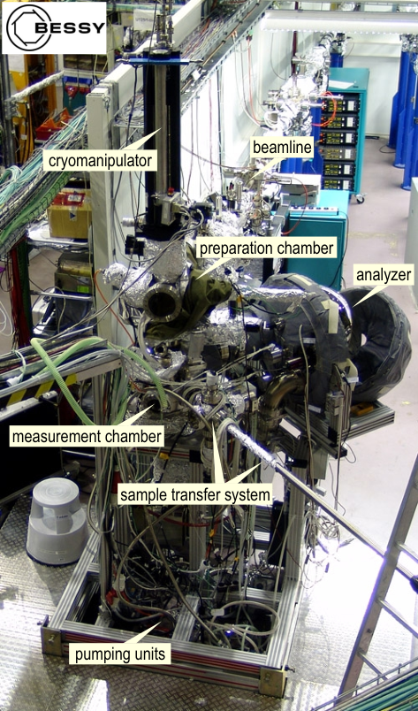
Experimental geometry. The analyzer is attached to the measurement chamber, which is connected to the beamline and is pumped to the ultra-high vacuum of mbar in order to prevent degradation of the sample surface during the experiment. The optical axis of the analyzer and the photon beam are aligned at 45∘ to each other in the horizontal plane in such a way that the view point of the analyzer coincides with the focus of the beam. The geometry of both experimental setups used in the present work is such that the entrance slit of the analyzer is placed vertically, i.e. perpendicular to the plane formed by the analyzer axis and the photon beam, as shown in Fig. 2.5. The investigated sample is fixed in the view point of the analyzer on a sample holder, which is in turn attached to the cryomanipulator that allows orienting the sample in three angular directions. In the following paragraph we will stop in more detail on the description of the manipulator and its functions. Except for the measurement chamber, the experimental setup normally includes a sample preparation chamber, supplied with a “fast entry” chamber for sample exchange. The appearance of the complete experimental setup can be seen in Fig. 2.6.
2.2.2 Cryomanipulator as a -space explorer

Figure 2.8: Transformation between the laboratory and intrinsic coordinate systems represented as three consecutive Euler rotations.
The function of the cryomanipulator is to position the sample precisely in the measurement chamber at an arbitrary position and angle while keeping it at a constant temperature between 30 and 400 K. In the present work, the Cryoax 6 manipulator was used (Fig. 2.7), with 3 rotational and 3 translational degrees of freedom, and reproducibility of the angles better than 0.2∘. The temperature of the sample, cooled by liquid He, can be controlled by a temperature sensor attached to the sample pocket.
To understand the need for the precise sample orientation, let us see what region of the momentum space can be measured by the analyzer in the vertical slit geometry for each particular orientation of the sample. We will introduce two orthonormal positively orientated coordinate systems: for the intrinsic coordinate system of the sample and for the laboratory coordinate system. The first one is fixed relative to the sample as shown in Fig. 2.1, with the axis normal to the sample surface and and axes corresponding to the high-symmetry directions of the sample. The second one is the laboratory coordinate system with the axis pointing along the optical axis of the analyzer, directed parallel to the entrance slit of the analyzer and lying in the horizontal plane so that is a right-handed orthogonal unit vector triplet (see Fig. 2.5).
The position of the intrinsic coordinate system relative to the laboratory coordinate system is uniquely determined by three Euler angles: polar angle , tilt , and azimuth . Starting from the laboratory coordinate system, the transformation to the intrinsic coordinate system can be represented as a composition of three consecutive rotations (see Fig. 2.8): first around the axis in the positive direction by the polar angle , then around the new (rotated) axis in the negative direction by the tilt angle , and finally around the new (twice-rotated) axis in the negative direction by the azimuthal angle . The coordinate transformation can be represented by the following matrix product:
| (2.15) |
The analyzer can detect only electrons with momenta in the laboratory coordinate system, where the analyzer angle is the angle between the electron momentum and analyzer axis limited by the acceptance angle, and is the absolute value of the free electron’s momentum. To find out the intrinsic coordinate representation of this vector, we substitute it into (2.15), which results in the following expressions for the sought and components of the momentum:
| (2.16a) | |||
| (2.16b) | |||
As follows from Eq. (2.5), the parallel components of the electron’s momentum are conserved during the photoemission process up to the multiples of the reciprocal lattice vector, so and in (2.16) actually represent the parallel components of the electron’s quasimomentum in the solid.
Figure 2.9: Position of the slit image in -space for different polar and tilt angles. The grid lines correspond to different values of the polar angle (vertical lines) and tilt (horizontal lines) at zero azimuth. Slit images for acceptance angle corresponding to different manipulator positions are shown in red. Non-zero azimuth would correspond to the rotation of the whole image by the azimuthal angle. Note that with the Cryoax 6 manipulator only tilt angles in the range from to are actually accessible.
The locus of all points that can be detected by the analyzer at a given manipulator position is called a slit image. It is a curve segment parametrically given by (2.16) as varies over the acceptance angle interval . Its position in -space can be changed by varying the manipulator angles (Fig. 2.9). Note that all the accessible vectors lie within a circle of radius , and the length of the slit image, i.e. the distance between momenta corresponding to the maximal and minimal analyzer angles, is given by . Both depend on the electron’s kinetic energy which in turn depends on the photon energy. Therefore by increasing the photon energy one can increase both the accessible momentum space and the momentum coverage of the slit image. On the other hand, the energy resolution will deteriorate with increasing photon energy.
-space mapping technique. As seen from Fig. 2.9, with the change of the polar angle the slit image moves orthogonally to itself, whereas with the change of the tilt angle the slit image moves parallel to itself. A change of azimuth is equivalent to the rotation of the slit image relative to the origin of coordinates. One sees that by changing the polar angle in small steps one can map a certain band in -space of the width of the slit image, which is called a polar map. Measuring several polar maps at different values of the tilt one can extend the width of the measured band of the -space. The direction, in which the polar mapping is performed, is given by the azimuthal angle. Sometimes it is convenient to perform mapping along different directions, e.g. along all high-symmetry directions of the sample. The movement of the manipulator responsible for the mapping can be performed automatically, resulting in a single three-dimensional data set of the photocurrent as a function of kinetic energy, analyzer angle, and manipulator angle. After rescaling the data according to (2.16) one ends up with a spectrum in the coordinates of binding energy and two projections of the momentum. As was shown in the previous section, such spectrum can be described within a number of approximations by Eq. (2.14) and can therefore provide important information about the single-particle spectral function of the sample.
2.2.3 Synchrotron light sources
Synchrotron: SLS BESSY II Electron energy: 2.4 GeV 1.7/1.9 GeV Circumference: 288 m 240 m Beamline: SIS X9L UE112-PGM1 UE112-LowE PGMb Energy range linear horizontal: 10 – 800 eV 15 – 600 eV 5 – 250 eV linear vertical: 100 – 800 eV — — circular: 50 – 800 eV — in project Beam spot size: m — slitsize m Resolving power: Undulator: UE212 UE112 UE112 Table 2.2: Comparative technical characteristics of the synchrotrons and beamlines used in the present work.

Modern ARPES experiments require high-quality light sources with high energy resolution (narrow bandwidth), variable photon energy and polarization, small spot size, high intensity, and high stability of the beam. All these conditions can be met only with synchrotron radiation at the built-on-purpose beamlines specially optimized for this class of experiments. The working principle of synchrotron light sources is based on the fact that high-energy charged particles (such as electrons, protons, or positrons) emit electromagnetic radiation in the ultra-violet to X-ray range when subjected to large accelerations orthogonal to their velocity [89, 90, 91]. The electrons are accelerated in a linear accelerator (linac) and then in the booster to energies of several GeV and then injected into the storage ring (see Fig. 2.11). The closed trajectory of the electrons is controlled by a set of bending magnets, and the energy losses at each revolution are compensated by the radio frequency cavity. To produce an intense photon beam, the electrons are led through undulators — special devices with a periodic pattern of the magnetic field. The undulators can be tuned to have a maximum of photon emission at a given energy (fundamental mode). Due to the relativistic effects the directional pattern of photon emission is peaked in the forward direction of the electron beam and is further enhanced by interference effects between photons emitted at different undulator wiggles. The photon beam generated in the undulator is then fed into one of several beamlines, where it is monochromatized and focused before it reaches the measurement chamber.
The data for the present work has been acquired at two electron synchrotrons (Fig. 2.10): at the SIS-9L beamline of the Swiss Light Source (SLS) in Villigen, Switzerland [92], and at the Berliner Elektronenspeicherring-Gesellschaft für Synchrotronstrahlung m. b. H. (BESSY) in Germany, beamlines UE112-PGM1 and UE112-LowE PGMb [93, 94]. All three beamlines are fitted with the plane grating monochromators (PGM). The summary of technical characteristics of the synchrotrons and the beamlines can be found in table 2.2.
![[Uncaptioned image]](0807.1434v1/Synchrotron.png) Figure 2.11: Sketch of a synchrotron facility with an ARPES end-station.
Figure 2.11: Sketch of a synchrotron facility with an ARPES end-station.
2.2.4 Sample preparation
In the present work, cuprates of the Bi2212 and Y123 families were studied (for the crystal structure, see section 3.1). The single crystals of the slightly overdoped (Bi, Pb)2Sr2CaCu2O8+δ ( K), slightly underdoped (Bi, Pb)2Sr2Ca1-xTbxCu2O8 and optimally doped Bi2Sr2CaCu2O8+δ were grown by the self-flux method in the group of Dr. H. Berger.†††† †† Institut de Physique de la Matière Complexe, Lausanne, Switzerland. The nearly optimally doped untwinned YBa2Cu3O6.85 ( K) samples were synthesized by the solution-growth method in the group of Prof. B. Keimer.‡‡‡‡ ‡‡ Max-Planck-Institut für Festkörperforschung, 70569 Stuttgart, Germany. Detwinning was achieved by applying a uniaxial mechanical stress to the sample at elevated temperatures.
Sample cleavage. Because ARPES is a surface-sensitive technique, the bulk samples need to be prepared by cleaving in situ in UHV conditions ( mbar) immediately before the measurement. At such vacuum conditions, the samples can usually be measured within approximately 24 hours after cleavage without any significant degradation of the surface. In order to transfer a sample into the UHV chamber and cleave it, it has to be glued to the sample holder as seen in Fig. 2.7 using a conducting silver epoxy glue.
![[Uncaptioned image]](0807.1434v1/Cleavage.png) Figure 2.12: Cleavage methods of BSCCO and YBCO samples and the typical LEED images taken from the cleaved surfaces.
(a) BSCCO samples can be cleaved with an O-shaped stripe of a sticky tape. (b) YBCO samples
have to be cleaved with an aluminum top-post glued to the top. (c) Transfer of a sample into the
preparation chamber for cleavage.
Figure 2.12: Cleavage methods of BSCCO and YBCO samples and the typical LEED images taken from the cleaved surfaces.
(a) BSCCO samples can be cleaved with an O-shaped stripe of a sticky tape. (b) YBCO samples
have to be cleaved with an aluminum top-post glued to the top. (c) Transfer of a sample into the
preparation chamber for cleavage.
In case of a BSCCO sample, weak Van-der-Waals bonds between the BiO layers make cleavage especially easy. It can be done simply with an O-shaped stripe of a sticky tape glued to the free surface of the sample as shown in Fig. 2.12 (a). In the UHV chamber, the stripe is then removed by the “fork” of the sample transfer system together with the upper layers of the crystal, which usually results in an atomically clean, mirror-like surface. The lower image in panel (a) shows a typical low-energy electron diffraction (LEED) picture taken from the surface of a Pb-free Bi2212 sample after cleavage.
Cleavage of YBCO samples requires a little more effort, but is also straightforward. As a rule, an aluminum top-post is glued to the free surface of the sample using the same silver epoxy glue, as shown in Fig. 2.12 (b). The top-post is tied to the sample holder with a thin golden wire in order to keep it from falling after cleavage. After the sample is transferred into the preparation chamber [see panel (c) of the same figure], the top-post is kicked off with a screwdriver, which usually results in at least part of the sample to have a mirror-like atomically clean surface suitable for measurements. Such method of cleavage allows one to apply a substantial cleaving force, which makes it possible to cleave even harder samples, such as LSCO, with a significantly non-zero chance of success.
2.2.5 Experimental data preprocessing
Intensity normalization. Possible inhomogeneities of the detector sensitivity in different momentum channels can lead to a slight -dependent intensity modulation in the raw ARPES spectra. Moreover, when measuring an angular map, the intensity may vary from one momentum cut to another due to various reasons. To eliminate these effects and to bring all spectra to a single intensity scale, the spectra are usually normalized to the background intensity integrated above the Fermi level. This spectral weight comes from the non-dispersing core levels excited by the higher harmonics of the synchrotron radiation, and is therefore expected to have no significant dependence on momentum. The normalized ARPES intensity is therefore given by
| (2.17) |
where is a kinetic energy window above the Fermi level: .
Energy scale corrections. The energy scale of a raw ARPES spectrum represents the kinetic energy of photoelectrons, which still has to be transformed to the binding energy scale. Naively, one could expect to be able to do the transformation using the energy conservation law . Unfortunately, this is not possible, because the work function is not known with the required precision. Instead, a reference spectrum of a freshly evaporated silver or gold film has to be measured, which is known to produce a perfect Fermi step. Because of the electrical contact between the sample, silver film, and analyzer, the Fermi levels in both spectra should coincide. can be therefore determined from the reference spectrum in every momentum channel independently (usually with subsequent smoothing**** ** For more details, see Ref. [95], p. 38 – 39.), and the energy scale transformation takes the form
| (2.18) |
The momentum-dependence of the Fermi energy determined in such a way comes mainly from the imperfectness of the energy calibration curves and the form of the analyzer slit. By the described procedure these deviations can be eliminated, which results in the accuracy of the energy scale 1 meV. For the best accuracy, it is important that the reference spectrum is taken with exactly the same experimental settings (analyzer slit, beamline settings, pass energy, etc.) as the spectra that are to be calibrated. For example, changing the photon energy of the beamline to a different value and back may result in an apparent shift of the Fermi level due to the imperfect reproducibility of the monochromator, so the reference spectrum will have to be remeasured.
Chapter 3 Electronic structure and renormalization effects in Bi2Sr2CaCu2O8+δ
3.1 Crystal structure of layered cuprates
3.1.1 Basic cuprate families
After the high-temperature superconductivity had been discovered in BaxLa5-xCu5O5(3-y) [1], the high- cuprates became one of the most studied materials in all of science, yielding in the research activity perhaps only to silicon. Even though the physics of superconductivity in these materials is not yet fully understood, their studies have been regularly producing new fundamental results in physics for more than 20 years since their discovery in 1986.
Figure 3.1: Crystal structure of the parent compounds for the three most studied families of high- cuprates:
LSCO, YBCO, and BSCCO, shown in chronological order of their discovery. The size of the atoms represents their
atomic radii. The perovskite-like oxygen coordination of Cu atoms is marked by the blue polyhedra. The lattice
parameters , , and are shown beside each drawing. Note that LSCO has a single CuO2 layer per
formula unit, while YBCO and BSCCO have a CuO2 bilayer per formula unit. The unit cells of LSCO and BSCCO
consist of two formula units shifted by , while the unit cell of YBCO
consists of a single formula unit.
![[Uncaptioned image]](0807.1434v1/CrystalStructure.png)
The crystal structure of the parent compounds for the three most actively studied families of cuprates is shown in Fig. 3.1. Among them, the La-based family, including La2-xBaxCuO4 (‘Zürich oxide’, LBCO) and La2-xSrxCuO4 (LSCO), was the first to be discovered [1, 96]. These are the hardest of the three materials, which makes the growth of larger single crystals ( 1 cm) possible. On the other hand, the stronger chemical bonds complicate the cleavage, making it difficult to obtain atomically flat surfaces for surface-sensitive measurements.

The second family of compounds, YBa2Cu3O7-δ (YBCO, or Y123), was also discovered within a year after the discovery of high- superconductivity [98, 99]. Unlike LSCO, it was a bilayer cuprate, and was the first superconductor to break the 77 K (liquid nitrogen) temperature limit. YBCO can be prepared in relatively large, clean, highly ordered single crystals, which makes it the best cuprate for studies by bulk-sensitive techniques such as INS. YBCO crystals are easily cleavable along the CuO chain layer. Unfortunately, such cleavage leads to the charge redistribution at the surface and, as a result, to significant overdoping of the upper CuO2 bilayer [100], precluding the studies of its bulk properties by surface-sensitive techniques such as ARPES. Note the slight orthorhombic distortion (1.8%) in the CuO2 planes of YBCO due to the anisotropy caused by the presence of the one-dimensional CuO chains.
The third compound, Bi2Sr2CaCu2O8+δ (BSCCO, or Bi2212), was independently discovered in 1988 by several groups [101, 102, 103, 104, 105] to become the first high-temperature superconductor not containing a rare earth element. It is usually available in thin, small single crystals, but is easily cleavable and is therefore the favorite material for STM and ARPES. Unlike YBCO, BSCCO has no chain layers, which makes its spectra easier to analyze. The cleavage happens symmetrically along the weakest bonds between the BiO layers and does not therefore distort the nearest CuO2 bilayers, so that they can be considered representative of the crystal’s bulk properties. On the other hand, because of the small volume of the samples, the bulk-sensitive measurements of BSCCO are rather difficult.
Figure 3.3: Schematic doping phase diagram of electron- and hole-doped high- superconductors showing, in particular, the superconducting (SC) and antiferromagnetic (AF) phases [106].
3.1.2 Periodic lattice modulations
The unit cell of BSCCO, shown in Fig. 3.1, is not exactly tetragonal. Within the -plane, there is a slight periodic distortion of the lattice. First, there is a commensurate lattice modulation in the direction as shown in Fig. 3.2 (a) that changes the original tetragonal unit cell to a larger orthorhombic unit cell [107, 108, 109, 110] with lattice parameters 5.414 Å, 5.418 Å, and 30.89 Å. If one nevertheless considers the original (pseudotetragonal) unit cell, in the reciprocal space this periodic modulation will manifest itself as shadows of the main bands shifted by (), as shown in Fig. 3.2 (b) and (d). Moreover, there is an incommensurate lattice modulation in the direction with a period of 4.75 [111, 112, 113], clearly observed both in surface- [102, 103, 114, 115] and bulk-sensitive [113] experiments. This modulation leads to the appearance of superstructure replicas in the ARPES spectra as shown in Fig. 3.2 (c) and (e), which are an additional obstruction for data analysis [116, 117, 118, 119]. To minimize their effect, BSCCO is often doped by Pb, which partially replaces the Bi atoms in the lattice, enhancing the [104] and removing the superstructure distortion [120, 121, 122, 123]. The Fermi surfaces in Fig. 3.2 (d) and (e) were measured from BSCCO crystals with and without Pb doping respectively.
![[Uncaptioned image]](0807.1434v1/Images/CupratesZoo.jpg)
3.1.3 The phase diagram
The layered structure of cuprates makes their electronic structure quasi-two-dimensional. Their parent compounds at zero doping are antiferromagnetic Mott insulators at half-filling (one hole per Cu site). The superconductivity and metallic behavior set in when the crystals are doped either by holes or electrons, as can be seen in the schematic phase diagram in Fig. 3.3 [106, 125, 126]. As more holes are added into the CuO2 planes, the O 2p5 and Cu 3d9 orbitals hybridize into the so-called Zhang-Rice singlet state [127], which leads to the antiferromagnetic superexchange between O and Cu holes. In the metallic and superconducting regimes the conduction bands are formed exclusively by the states within the CuO2 planes (in case of YBCO also by the CuO chains). The superconductivity occurs only within the CuO2 planes, whereas the rest of the crystal structure serves as a charge reservoir to control the doping of the planes.
3.1.4 Variety of high- cuprates
In Ref. [124], H. Eisaki et al. provide a classification of the hole-doped cuprates in terms of the disorder site and the number of CuO2 layers, which is shown in table 3.1, together with the corresponding critical temperatures. Note that increases both across the rows and down the columns of the chart for each single family of materials, each denoted by a different color. By changing the number of layers, the disorder atom and its position, dopants, etc. the macroscopic properties of the high- cuprates, including , can be significantly optimized. In most recent attempts to increase , crystals with the so-called planar weight disparity** * Planar weight disparity exists whenever planes within the layered perovskites are alternated light-heavy. (PWD) [128, 129] were prepared, some of which are claimed to exhibit signatures of superconductivity at temperatures as high as 175 K at ambient pressure [129].
3.2 Electronic band dispersion and self-energy
3.2.1 Electronic structure of Bi2212 as seen by ARPES
![[Uncaptioned image]](0807.1434v1/ElectronicStructure.png) Figure 3.4: (a) Schematic dispersion of the conductance band of optimally doped Bi2212 in a tight-binding model
(parameters from Ref. [130]). The bonding and antibonding sub-bands are shown in pink
and yellow color respectively. (b) LDA band structure of Bi2Sr2CaCu2O8.3 along the
high-symmetry directions from Ref. [131]. (c) and (d) Typical ARPES
images measured in the vicinity of the antinodal and nodal points in the directions shown in panel (a) by the
red arrows. The color scale represents photoemission intensity.
Figure 3.4: (a) Schematic dispersion of the conductance band of optimally doped Bi2212 in a tight-binding model
(parameters from Ref. [130]). The bonding and antibonding sub-bands are shown in pink
and yellow color respectively. (b) LDA band structure of Bi2Sr2CaCu2O8.3 along the
high-symmetry directions from Ref. [131]. (c) and (d) Typical ARPES
images measured in the vicinity of the antinodal and nodal points in the directions shown in panel (a) by the
red arrows. The color scale represents photoemission intensity.
Due to the layered crystal structure with the conductance electrons confined to the CuO2 planes, the electronic structure of the high- cuprates is quasi-two-dimensional, which significantly simplifies the ARPES measurements and data treatment. Though a small but finite -dispersion has been reported [132, 133, 134, 135], much of the existing ARPES work on the cuprates implicitly assumes the system to be perfectly two-dimensional [65, 136], ignoring the effects of interlayer hopping.
As mentioned earlier, the conductance band of a doped CuO2 plane is formed by the hybridized O 2p5 and Cu 3d9 states — the Zhang-Rice singlet [127]. In a solitary CuO2 layer, this state corresponds to a single band in the momentum space, whereas in the double-layer compounds it is additionally split into the bonding and antibonding sub-bands [137, 138, 139, 140] due to the non-zero interaction between the layers. The dispersion of the conductance band in Bi2212 at optimal doping is schematically presented in Fig. 3.4 (a) (only the occupied states below the Fermi energy are shown). As illustrated in the figure, the Fermi surface consists of the two hole barrels formed by the bonding and antibonding bands. The bilayer splitting is evident both from the local-density approximation (LDA) based band structure calculations [panel (b)] and from the experimental ARPES data [panel (c)]. As was already discussed in §3.1.2, the situation is additionally complicated by the shadow Fermi surface and superstructure replicas, possibly due to the periodic lattice modulations in these materials. The typical experimental Fermi surfaces of Bi(Pb)-2212 and Bi2212 can be seen in Fig. 3.2 (d) and (e).
3.2.2 Self-energy effects in the ARPES spectra of Bi2212
Figure 3.5: Real and imaginary parts of the self-energy (shown by blue and red double headed arrows respectively) on a photoemission image. Bare band dispersion (black solid line) and renormalized dispersion (red points). Red solid line represents the momentum distribution curve (MDC) taken at . The position of MDC maximum determines , and the momenta of its half-maximum level determine and . The figure is reproduced from Ref. [141].
Except for the electron dispersion, the spectral function measured by ARPES also contains information about the self-energy, which is reflected in the broadening of the spectrum and the deviation of the experimental dispersion from the bare band. Possibility to extract the self-energy from experimental data is of great importance, as it gives access to the understanding of interactions within the many-body system. The method of simultaneous self-consistent evaluation of the bare band dispersion and self-energy from ARPES spectra in the nodal direction has been developed in Ref. [130, 142, 143, 141] and will be discussed in detail in the next paragraph. It is remarkable that the dispersion vanishes at the nodal point [135], therefore there is no additional broadening introduced to the nodal spectrum due to the three-dimensionality, which is not the case at other points along the Fermi surface. This fact, as well as the maximal steepness of the dispersion, makes the self-energy analysis easiest at the node.
Neglecting for the moment the effects of the energy and momentum resolutions as well as the influence of matrix elements, one can consider the ARPES signal to be simply proportional to the spectral function, as follows from Eq. (2.14). The self-energy effect on the ARPES spectrum is then given by Eq. (1.34), which we can rewrite by taking the imaginary part and writing explicitly the real and imaginary parts of the self-energy as
| (3.1) |
Formula (3.1) is illustrated in Fig. 3.5. The background image (in gray scale) represents a typical nodal spectrum in the vicinity of the Fermi level. The red curve shows a constant energy cut, or momentum distribution curve (MDC) for a particular energy . The red dots mark the experimental dispersion, i.e. positions of MDC maxima taken at different . The solid black line is the bare band dispersion . Points and are the momenta at which MDCω reaches its half-maximum level (note that ). Then the real part of the self-energy is the deviation of the experimental dispersion from the bare band at , while the imaginary part is given by [141]
| (3.2) |
![[Uncaptioned image]](0807.1434v1/Kink.png) Figure 3.6: “Kink” in the experimental dispersion along the nodal direction in pure Bi2212. (a) Photoemission
intensity
distribution along the nodal direction. (b) Experimental dispersion (red dots). The solid black line
is a guide
to the eye. The figure is reproduced from Ref. [144].
Figure 3.6: “Kink” in the experimental dispersion along the nodal direction in pure Bi2212. (a) Photoemission
intensity
distribution along the nodal direction. (b) Experimental dispersion (red dots). The solid black line
is a guide
to the eye. The figure is reproduced from Ref. [144].
There are two major self-energy effects that can be observed experimentally along the nodal direction. First, the MDC width increases with at low energies, which is a typical behavior both for normal and marginal Fermi liquids (see §1.5.2). Then, there is an anomaly in the experimental dispersion, the so-called “kink”, at about 0.05 – 0.10 eV binding energy [145, 146, 147, 148, 149, 150, 144], as shown in Fig. 3.6. According to the most common understanding, this energy scale is a result of the bosonic mode coupling term in the self-energy (see §1.5.3) that originates from coupling either to a phonon [147, 148] or a collective mode of electronic origin [146, 149, 150, 144]. In the following, we will consider the two constituents of the self-energy in more detail.
![[Uncaptioned image]](0807.1434v1/AntinodalSpectra.png) Figure 3.7: Renormalization in the antinodal region of -space. Left: data taken with a photon energy of
38 eV, at which the signal from the bonding band is maximal. Middle: data taken at 50 eV,
where the signal from the antibonding band is dominant. Right: subtraction of the latter from the former
yielding the spectral weight of the bonding band. The figure is reproduced from
Ref. [151].
Figure 3.7: Renormalization in the antinodal region of -space. Left: data taken with a photon energy of
38 eV, at which the signal from the bonding band is maximal. Middle: data taken at 50 eV,
where the signal from the antibonding band is dominant. Right: subtraction of the latter from the former
yielding the spectral weight of the bonding band. The figure is reproduced from
Ref. [151].
As one moves away from the nodal point towards the antinode [146, 151], the situation is complicated by the opening of the superconducting gap, smaller band width, stronger renormalization, and non-zero -dispersion, which leads to an additional broadening of the spectrum, precluding exact quantitative self-energy analysis in this region of the momentum space. Nevertheless, the signatures of the renormalization similar to those at the nodal point can be clearly observed, as seen from Fig. 3.7. As the renormalization becomes stronger towards the antinode, the spectral weight becomes “squeezed” between the superconducting gap energy and the energy of the bosonic mode, significantly reducing the band width. For comparison, see the model spectra from Fig. 1.2.
3.2.3 Self-consistent evaluation of the bare dispersion and self-energy
Let us now return to the analysis of nodal spectra and scrutinize the procedure for extraction of the self-energy from photoemission data [130, 142, 143, 141, 152]. As follows from Eq. (3.2), the extraction of the imaginary part is straightforward if one knows the dispersion of the bare band. One has then simply to fit each MDCω with some, generally speaking, asymmetric lineshape, determine momenta at which the fitting curve reaches its half-maximum level, and substitute them into (3.2).
Unfortunately, the bare band dispersion is usually not known with the required accuracy. Though band structure calculations can provide us with the bare electronic structure, it is a priori unknown whether these results can be relied upon. It is therefore desirable to be able to extract the bare band dispersion from the experimental data together with the self-energy. This becomes possible, if we make some assumptions about the functional form of the dispersion. As soon as we analyze the electronic structure in the vicinity of the Fermi level, it is a good approximation to assume that the dispersion has a parabolic shape given by
| (3.3) |
The Fermi momentum is simply determined as the crossing point of the experimental dispersion with the Fermi level. We are therefore left with a single free parameter .
Imaginary part (). For a quadratic dispersion, formula (3.2) can be rewritten as
| (3.4) |
where is the half-width at half-maximum (HWHM) of the MDC peak. The last equality follows from the following property of a parabolic function: if , then .
There is another useful consequence of this property. It is interesting that the ratio , where , is identical to unity in case of a parabolic dispersion, i.e. . We can rewrite this equality as
| (3.5) |
The left part of (3.5) characterizes the asymmetry of the MDC peak. Indeed, the position of the peak maximum deviates from the center of the interval by . The ratio then gives an estimate of the relative error that one introduces by neglecting the asymmetry of the peak. On the other hand, in the vicinity of the Fermi level the right part of the same equation (3.5) is of the order of . This observation leads us to a useful conclusion: it is often sufficient to use a symmetric line shape in the fitting procedure (e.g. a Lorentzian or Voigt profile), as long as (which can be called low-energy region). As a rule of thumb, this approximation holds approximately half-way down to the bottom of the band, i.e. down to 0.5 eV binding energy. At energies that high, the parabolic approximation for the bare band dispersion probably breaks down as well, so taking the asymmetry of the peak into account is not expected to improve the accuracy of the self-energy analysis procedure, at least in this simple model. Moreover, our analysis is essentially based on the assumption that the self-energy is a function of one variable, which is justified only if the spectral function is well localized in momentum (see §1.5.1). It should be therefore emphasized that the described procedure is only capable of studying the behavior of the self-energy in the low-energy region, but not in the vicinity of the band bottom.
Relation to the real part (). Formula (3.4) gives the imaginary part of the self-energy in the assumption of the parabolic bare band. We can replace the unknown constant by the Fermi velocity of the bare band . A similar expression can be written down for the real part of the self-energy in the same approximations, which leads to
| (3.6a) | ||||
| (3.6b) | ||||
The real and imaginary parts of the self-energy are related by the Kramers-Kronig transformation (1.35), which will let us determine the unknown factor in formulae (3.6). In order to perform the Kramers-Kronig transformation, the experimentally extracted self-energy curves have to be symmetrized to the unoccupied part of the spectrum () and extrapolated to the high-energy region using some empirical model of the ‘tails’, for example:
| (3.7) |
The constants and are determined in a way such that the ‘tails’ are smoothly joined to the experimental data. The value of usually provides a reasonable result, while the cut-off energy can be either treated as an independent fitting parameter, or chosen from the following rule of thumb: [143]. This energy approximately corresponds to the point where reaches its maximum and starts to decrease, while crosses zero.
The fitting procedure is done in three steps. In the first two steps, the real part of the self-energy, for given and , is calculated in two independent ways: (i) determined directly from Eq. 3.6a; (ii) calculated indirectly from Eq. 3.6b with subsequent Kramers-Kronig transform. Then, in step (iii), the fitting parameters are adjusted to minimize the difference . The real and imaginary parts are considered to be Kramers-Kronig consistent, if this can be done with a reasonable accuracy determined by the experimental resolution.
Figure 3.8: Real and imaginary parts of the self-energy extracted from the experiment with the described procedure. Figure reproduced from Ref. [143].
Influence of the experimental resolution. It should be mentioned that the imaginary part of the self-energy determined from experimental data is affected by the experimental resolution. This influence can be approximated by the following formula:
| (3.8) |
where the empirical parameter characterizes the overall resolution. The frequency-dependent contribution of the resolution to the imaginary part of , which we will call here the resolution function, is then given by
| (3.9) |
Due to the linearity of the Kramers-Kronig transform, the contribution of the resolution function to the real part of the self-energy will be simply given by the Kramers-Kronig transform of .
Returning to the fitting procedure described above, note that is not influenced by the resolution function, therefore the difference has to be fitted not to zero, but to the real part of the resolution function (Fig. 3.8). For details, see Ref. [143].
A more subtle way to account for the experimental resolution is to use the Voigt profile for MDC fitting [152]. As the intrinsic MDC line shape is a Lorentzian, and the resolution effect is equivalent to Gaussian broadening, such procedure allows one to separate the intrinsic line width from the resolution effect.
Tight-binding model. The above-described procedure allows one to determine the energy scale of the band structure, i.e. either or the nodal Fermi velocity . In Pb-Bi2212, their values are 0.860.03 eV and 2.460.07 ÅeV respectively [143]. With this information at hand, the whole band structure can be fitted by a tight-binding model to the experimentally measured Fermi surface map. The Fermi surface shape is reproduced by fitting the dimensionless tight-binding parameters to the Fermi surface map, and the energy scale is taken from the self-consistent self-energy analysis. This procedure is justified, as the real part of the self-energy is zero at the Fermi level, so the photocurrent is localized along the Fermi surface given by the bare band structure.
We will use the tight-binding model limited to the three nearest neighbor intraplane hopping terms and one interlayer hopping term that is responsible for the bilayer splitting. Rewriting the expression (1.12) for the pseudo-tetragonal crystal lattice of Bi2212, one gets the following model for the dispersion [130]:
| (3.10) |
In Ref. [130], this model has been fitted to the experimental ARPES data from two Bi2212 samples with different doping: overdoped (=69 K) and underdoped (=77 K). The corresponding tight-binding parameters are given in table 3.2. In the following, we will use linear interpolation between these two samples to find the tight-binding parameters for the intermediate doping levels.
Sample (eV) (eV) (eV) (eV) (eV) OD 69 K 0.40 0.090 0.045 0.082 0.43 UD 77 K 0.39 0.078 0.039 0.082 0.29 Table 3.2: Tight-binding parameters of the Bi2212 conductance band from Ref. [130].
3.2.4 Models of the self-energy
Understanding the nature of the self-energy provides an insight into the many-particle interaction processes in the system. It is therefore essential not only to be able to evaluate the self-energy curves from experiment, but to understand the origin of its constituents. It turns out that the self-energy in cuprates can we well reproduced by a relatively simple model which involves two kinds of interactions: Fermi-liquid like component originating from the electron-electron interaction (see §1.5.2) and the second term which originates from the coupling to a bosonic mode (see §1.5.3), which we will denote here by and respectively [153]. The self-energy can be assumed to be the same for the bonding and antibonding bands, although strictly speaking, one should also account for the difference in scattering rates between the two bands [154], which is however small enough to be neglected in our case.
To reproduce the experimental data, we model the imaginary part of the self-energy, and calculate the real part by means of the Kramers-Kronig transformation. This is done independently in the nodal and antinodal directions, so that the self-energy at an arbitrary point can be found by a d-wave interpolation between the node and antinode:
| (3.11) |
Nodal direction. In the nodal direction, where the superconducting gap is zero and the partial density of states can be considered constant in the vicinity of the Fermi level, the electron-electron scattering rate is assumed to have a quadratic energy dependence typical for a normal Fermi liquid:
| (3.12) |
The electron-boson part is modeled as
| (3.13) |
This function is analogous to (1.78), but also takes into account the finite broadening of the bosonic mode, which is given here by the empirical parameter . In the limit , this corresponds to a step in the nodal scattering rate at the energy with amplitude .
The broadened bosonic mode, as introduced in (3.13), is well localized in energy, i.e. it has exponentially decaying tails. This formula is purely phenomenological, as in practice the exact shape of the bosonic spectrum is difficult to account for. Another possible way to introduce the broadening of the mode would be to offset the pole in the real part of the self-energy (1.78) [53]:
| (3.14) |
where is a small broadening parameter. Though this might seem to be a more natural way, it is not very convenient in practical situations because of the slowly decaying tails, which produce nonzero scattering rate near the Fermi level.
The total scattering rate is calculated from the two constituents by the following formula:
| (3.15) |
The denominator is necessary to guarantee convergence of the Kramers-Kronig transformation and represents a special case of the ‘tails’ model (3.7) for . In Ref. [153] the cutoff energy was chosen to be one third of the bare band bottom energy .
Antinodal direction. In the antinodal direction, the situation is more complicated, because the partial density of states can no longer be considered constant in the superconducting state. Due to the nonzero energy gap, the density of states develops a pile-up peak, which can be directly observed in scanning tunneling spectroscopy experiments [106, 155, 156]. Ref. [156] provides a convenient model for the partial density of states, which is
| (3.16) |
where is the superconducting gap and is a broadening parameter (see Ref. [156] and references therein).
Figure 3.9: The Kramers-Kronig consistent real and imaginary parts of the nodal and antinodal self-energies. The figure is reproduced from Ref. [153].
The electron-electron scattering rate will be then proportional to the number of states above the energy squared:
| (3.17) |
where is the maximal superconducting gap at the () point. The bosonic part can be approximated by
| (3.18) |
Here is the energy of the mode and is the broadening parameter at antinodal point.
We assume the particle-hole symmetry in to evaluate the self-energy in the unoccupied part of the spectrum (), so that the real and imaginary parts of the self-energy are odd and even functions of energy respectively.
Fitting procedure. In the nodal direction, the self-energy model can be directly fitted to the experimentally measured self-energy. At the antinode, this is not possible, so one has to calculate the spectral function from the self-energy (see section 3.4) and compare it to the experimentally observed one to achieve a good correspondence between the two. This was done in Ref. [153], where all the free parameters were adjusted during comparison with a set of ARPES spectra of Bi2212 to achieve the best correspondence. The resulting self-energies are plotted in Fig. 3.9. The best-fit parameters of the model are listed in the following table:
| eV-1 | meV | meV | meV |
|---|---|---|---|
| meV | meV | meV |
3.3 Superconducting energy gap
3.3.1 Momentum-dependence of the gap
Before proceeding to the description of the Green’s function model, which will be the main result of this chapter, we need to pause for a more detailed discussion of the superconducting energy gap and its evaluation from the ARPES data. As we know from BCS theory (§1.4.1), the gap function is the order parameter of the superconducting phase transition. The question of the symmetry of the superconducting gap has therefore become a hot topic in high- superconductivity research and is crucial to understand the nature of superconductivity in cuprates [157, 158, 159]. Though there are still hot debates about the exact behavior of the gap as a function of momentum [160, 161, 162, 163, 164, 165, 166, 167], temperature [167, 168, 169, 170, 171], doping [172, 173, 174, 175], and its space variations [115, 176], it is now well established that the order parameter, and therefore the pairing interaction, have a predominantly symmetry of the gap in the superconducting state [177, 159, 178, 179, 180]:
| (3.19) |
possibly with a minor s-wave component [181]. Such momentum-dependent order parameter is one of the major distinctions of the high- cuprates from conventional superconductors, where the gap has an s-symmetry and is therefore -independent. Though some data suggest that (3.19) might be incomplete and that higher order terms might also be present in the momentum-dependence of the gap function at low doping [173, 182], for the purposes of the present work it is a good approximation to consider the gap as having a perfect d-wave shape.
3.3.2 Evaluating the gap from ARPES data
One has to draw a clear distinction between the gap function , which is defined for all values of and enters the Green’s function of the superconducting state (1.66), and the energy gap extracted in a photoemission experiment [183, 184, 161, 179, 185, 186, 138, 130], usually defined as the leading edge gap (LEG) [185, 186, 138, 130] and measured along the Fermi surface contours. The leading edge gap is determined as the lowest binding energy at which the energy distribution curve (EDC) reaches half of its maximum. It is understandable, and usually admitted, that the LEG should depend on any parameters that determine the EDC line shape and, unless the relation between the LEG and the real gap is known, can be considered only as a qualitative representation of the real gap. So, analyzing the experimental data it is very important to distinguish between the artificial variations of the LEG and changes caused by the real gap in the electronic density of states. We will not stop here on the details of the LEG behavior as a function of experimental parameters, which can be found in Ref. [130]. Instead, we will consider a couple of examples in which the momentum dependence of the LEG is revealed from ARPES data analysis.
(a)![[Uncaptioned image]](0807.1434v1/Gap1.png) (b)
Figure 3.10: Plots of the LEG anisotropy as a function of the Fermi surface angle within the quadrant of the
Brillouin zone [see inset at the bottom of panel (b)]: (a) for a nearly optimally doped Bi2212 sample
measured at 13 K [179]; (b) for an underdoped Bi2212 sample measured at 120 K (above
the transition temperature) in the pseudogap phase [187].
(b)
Figure 3.10: Plots of the LEG anisotropy as a function of the Fermi surface angle within the quadrant of the
Brillouin zone [see inset at the bottom of panel (b)]: (a) for a nearly optimally doped Bi2212 sample
measured at 13 K [179]; (b) for an underdoped Bi2212 sample measured at 120 K (above
the transition temperature) in the pseudogap phase [187].
It is clear that in case of a non-zero energy gap, the spectral weight at the Fermi level vanishes and the Fermi surface is therefore no longer defined. One can however redefine it as the locus of points where the LEG reaches its minimum [130, 187, 97]. This permits plotting the gap as a function of the Fermi surface angle, measured from the center of the barrel. In Fig. 3.10 two such dependencies are shown for a nearly optimally doped Bi2212 sample at low temperature [panel (a)] and for underdoped Bi2212 sample above the transition temperature in the pseudogap phase [panel (b)]. In the first panel, only points measured along the minimal gap locus are shown. In the second case, all momenta are plotted, so that the actual -dependence of the pseudogap is represented by the low-gap envelope curve of all data points. In panel (a), the angular variation of the gap is in excellent agreement with that expected from a d-wave order parameter of the form. In the pseudogap case (b), significant deviations from this shape are observed.
3.4 Modeling of the Green’s function
3.4.1 Normal Green’s function in the superconducting state
The self-energy obtained in §3.2.4 can be used to model the Green’s functions — a fundamental result that can be used in a variety of different calculations and enables comparisons of ARPES with other experimental methods, as will be shown in chapter 5. It is tempting to use the raw ARPES data for such calculations, which is however unreliable. The problem is that the measurements are strongly affected by matrix element effects, as will be demonstrated in the next chapter, by the experimental resolution, and possibly some experimental artifacts [188], such as intensity variations during measurements, normalization procedure applied to the data, etc. Experimental spectra include contributions from both bonding and antibonding bands that are difficult to separate in a wide range of momenta. The spectral function originally measured by ARPES also lacks the absolute intensity scale, which precludes quantitative calculations.
Instead, in Ref. [153] we have employed a model of the Green’s function based on the bare electron dispersion studied in Ref. [130] and a model for the imaginary part of the self-energy described in §3.2.4. The Green’s function was then calculated according to [189]:
| (3.20) |
where is the superconducting d-wave gap (3.19) changing from zero along the Brillouin zone diagonals to the maximal value of along the antinodal directions. The term in the denominator of (3.20) is the anomalous vertex function,†† † The superconducting gap in BCS theory is the solution of [190]. Alternatively to and , one can introduce the complex effective mass function, , and the complex effective gap function [191, 192]. which is related to the pairing gap and is generally energy-dependent [189, 193, 190, 194, 195, 192, 191], though its energy dependence is often neglected [189].
To achieve the best reproduction of the experimental data, all the free parameters of the self-energy were adjusted during comparison with a set of ARPES spectra of Bi2212 to achieve the best correspondence (see Fig. 3.11 for the comparison of the model with experimental spectra and the table on page 3.2.4 for the fitting parameters). It is worth stressing that a simple self-energy model that includes coupling only to a single bosonic mode can accurately reproduce the state of the art ARPES spectra of Bi2212, as Fig. 3.11 clearly shows.
![[Uncaptioned image]](0807.1434v1/Model.png) Figure 3.11: Comparison of the model with experimental ARPES spectra of optimally doped Bi2212 at 30 K taken with 50 eV
(a, b) and 38 eV
(c) photon energies. The model spectra are smoothed with a Gaussian to account for 20 meV energy resolution
and
0.025 Å-1 angular resolution. (a) Spectra at the point with the corresponding
energy
distribution curves (below) taken along the dashed lines. (b) Nodal spectra along the
direction. (c) Comparison of the experimental and model spectra taken at an intermediate position in
-space to check the validity of the interpolation of the self-energy between the nodal and antinodal
directions. (d) The Kramers-Kronig consistent real and imaginary parts of the nodal and antinodal
self-energies. (e) Positions of the cuts (a – c) in -space. The figure is
reproduced from Ref. [153].
Figure 3.11: Comparison of the model with experimental ARPES spectra of optimally doped Bi2212 at 30 K taken with 50 eV
(a, b) and 38 eV
(c) photon energies. The model spectra are smoothed with a Gaussian to account for 20 meV energy resolution
and
0.025 Å-1 angular resolution. (a) Spectra at the point with the corresponding
energy
distribution curves (below) taken along the dashed lines. (b) Nodal spectra along the
direction. (c) Comparison of the experimental and model spectra taken at an intermediate position in
-space to check the validity of the interpolation of the self-energy between the nodal and antinodal
directions. (d) The Kramers-Kronig consistent real and imaginary parts of the nodal and antinodal
self-energies. (e) Positions of the cuts (a – c) in -space. The figure is
reproduced from Ref. [153].
3.4.2 Anomalous Green’s function
As was shown in §1.4.2, the Green’s function of the superconducting state is actually a 22 spinor, which includes an anomalous off-diagonal element. The anomalous Green’s function can not be directly measured in an ARPES experiment, but with the self-energy and the pairing vertex present in the model (3.20), it becomes possible to calculate the anomalous Green’s function analytically [193]:
| (3.21) |
The described model of the Green’s functions is free of the disadvantages inherent in the raw ARPES data. Only in such a way can one completely separate the bonding and antibonding bands, which is impossible to achieve in the experiment. Besides the already mentioned absence of matrix element effects and experimental resolution, the formulae (3.20) and (3.21) also allow one to obtain both real and imaginary parts of the Green’s functions for all k and values including those above the Fermi level. It automatically implies the particle-hole symmetry () in the vicinity of the Fermi level, which in case of the raw data would require a complicated symmetrization procedure based on Fermi surface fitting, being a source of additional errors. Finally, it provides the Green’s function in absolute units, allowing for quantitative comparison with other experiments and theory, even though the spectral function originally measured by ARPES lacks the absolute intensity scale. Thereupon, we find the proposed analytical expressions to be better estimates for the self-energy and both Green’s functions and therefore helpful in calculations where comparison to the experimentally measured spectral function is desirable.
Chapter 4 Matrix element effects in photoemission spectra of cuprates
4.1 Manifestation of the photoemission matrix elements in an ARPES experiment
4.1.1 Excitation energy dependence of the matrix elements
Figure 4.1: The intensities of bonding and antibonding bands in an antinodal spectrum of Bi2212 as a function of excitation energy extracted from experimentally measured ARPES spectra. The figure is reproduced from Ref. [139].
In section 2.1 it was shown that ARPES essentially measures the one-particle spectral function of the initial states. Much of the data on the cuprates have been analyzed within this approximation. While this simple approach yields insights into the underlying physics, a satisfactory description of the spectra must necessarily model the photoexcitation process properly by taking into account the matrix element involved, the complex modifications of the wave functions resulting from a specific surface termination, and the effects of multiple scattering and of finite lifetimes of the initial and final states [196]. It is now well recognized [197, 198, 188, 139, 199, 196, 200, 201, 202, 203, 204, 205] that this interplay between the bulk and surface phenomena — the so called “matrix element effect”, is essential for a satisfactory interpretation of the ARPES data.
In a photoemission experiment, matrix elements manifest themselves as an additional modulation of the photocurrent with momentum, excitation energy, and polarization of the incident photons. On the one hand, such modulation is harmful, as it complicates data analysis and distorts the underlying electronic structure. On the other hand, it can be used to enhance or mask the ARPES signal from individual bands, for example bonding and antibonding, by tuning the excitation energy so that only one of the sub-bands is enhanced (see Fig. 3.7 as an example). It is therefore essential to know the behavior of the matrix elements depending on the experimental parameters in order to uncover the underlying electronic structure.
The relative contributions of the bonding and antibonding bands to the spectrum of Bi2212 taken near the antinodal point are known as a function of photon energy both from experiment [188, 139, 199] and theoretical calculations [200, 196, 201, 202, 203, 204, 205]. The experimentally measured intensity prefactors for the two sub-bands are shown in Fig. 4.1. One can see that 38 eV photons effectively excite electrons only from the bonding band, while the antibonding band is enhanced by 50 eV photons.
In the nodal direction, a similar quantitative measurement is complicated in Bi2212 because of the very small bilayer splitting [140]. But the modulations of the relative bonding/antibonding intensity have nevertheless been observed both in Bi2212 [140, Fig. 1 (d) – (g)] and in Y123 [206], though not quantified.
4.1.2 Momentum and polarization dependence of the matrix elements
The dependence of the photoemission matrix elements on momentum has been studied mostly at the Fermi level, i.e. as the variation of photocurrent intensity along the Fermi surface contours. Unfortunately, the published results of numerical calculations covering an extended region of -space are available only for a couple of excitation energies: 21.2 eV [119] and 22 eV [200, 196], and there are no systematic studies of the matrix element effects as a function of both photon energy and momentum, as well as at higher binding energies.
![[Uncaptioned image]](0807.1434v1/ZhangRice.png) Figure 4.2: Schematic of the Zhang-Rice singlet state in the one-particle representation. The Zhang-Rice
singlet has the same symmetry as a orbital, implying the existence of two mirror planes
perpendicular to the CuO2 plane, labeled M1 and M2. The black and white colors represent opposite signs of
the
orbital lobes. The figure is reproduced from Ref. [207].
Figure 4.2: Schematic of the Zhang-Rice singlet state in the one-particle representation. The Zhang-Rice
singlet has the same symmetry as a orbital, implying the existence of two mirror planes
perpendicular to the CuO2 plane, labeled M1 and M2. The black and white colors represent opposite signs of
the
orbital lobes. The figure is reproduced from Ref. [207].
Some conclusions about the behavior of the matrix elements can be made, though, even from simple symmetry and parity considerations. In the one-band Hubbard model, the - model and its extensions, the Zhang-Rice singlet state is a one-particle state that has the same symmetry as a Cu 3d orbital. Fig. 4.2 shows a schematic representation of the Zhang-Rice singlet state, including the two mirror planes M1 and M2 which are perpendicular to the CuO2 plane and which are relevant for photoemission along – and – respectively [207]. The wave function of the photoelectron to be detected by the analyzer must always be even with respect to the detector plane, otherwise it would be zero at the detector. The initial state (ground state) is a one-hole state with symmetry, and therefore has even parity with respect to M2 and odd parity with respect to M1. In the assumption of the Zhang-Rice singlet construction applicability to the first electron-removal final state, this state is totally symmetric. Let’s consider two possible polarizations of the incident photons: (i) polarization plane coincides with the emission plane (parallel polarization); (ii) polarization plane is orthogonal to the emission plane (perpendicular polarization). The photoemission operator has even () parity in a parallel and odd () parity in a perpendicular experimental geometry. The matrix element thus formally vanishes for the two cases:
| (4.1) |
Therefore along the – direction the first electron-removal state feature is expected to show the highest photoemission intensity with perpendicular geometry, whereas along – maximal intensities are to be observed in the parallel geometry. This simple consideration explains the strong momentum and polarization dependence of the matrix elements and demonstrates that in particular geometries the ARPES signal may completely vanish due to the symmetry selection rules.
4.2 Anomalous high-energy dispersion as a matrix element effect
4.2.1 “Waterfalls” in cuprates: first observations
Appearance of the new generation of electron spectrometers with the wide acceptance angle ( 15∘ for Scienta R4000) has opened up the possibility of viewing the electronic structure of cuprates over a broad momentum range covering more than one Brillouin zone** * Unlike the standard definition of the Brillouin zone in solid state physics, here by different Brillouin zones we mean primary and secondary cones of photoemission (Mahan cones), as introduced in Ref. [72]. in a single measurement. This has triggered a series of publications evidencing anomalous high-energy dispersion in the renormalized band structure of Bi2Sr2CaCu2O8+δ [208, 209, 210, 211, 212, 213, 214, 215], Bi2Sr2CuO6+δ [212, 213, 214, 215, 216], La2-xSrxCuO4 [215, 214, 217], La2-xBaxCuO4 [209], Pr1-xLaCexCuO4 [213], Ba2Ca3Cu4O8(OδF1-δ)2 [215], and Ca2CuO2Cl2 [218] at the binding energies higher than 0.3 – 0.5 eV — a region that has previously been scarcely explored. All of these reports seem to agree on the qualitative appearence of the spectra: (i) in the – (nodal) direction the “high-energy kink” (“giant kink”) at 0.4 eV is followed by a nearly vertical dispersion (“waterfall”) that ends up below 1 eV with a barely detectable band bottom approaching that of the bare band (see Fig. 4.3); (ii) the band bifurcates near the high-energy kink, forming another branch with a bottom at 0.5 eV [208, 213, 215]; (iii) some authors claim that the actual band width is even larger than that of the bare band, reaching 1.6 eV [212, 215]; (iv) as one moves away from the nodal direction, the “vertical dispersion” persists surprisingly up to the (antinodal) point, forming a “diamond” shape in momentum space at 0.5 eV [214, 209, 217] [Fig. 4.3 (b) and (c)].
These observations suggested the presence of new energy scales in the electronic structure. Except for the well-known “kink” at 0.05 – 0.10 eV, the second energy scale corresponding to the “high-energy kink” at 0.4 eV, and even a third energy scale at 0.9 eV [210] have been reported. It is widely believed that understanding the interplay between different energy scales in any physical system, and in high- superconductors in particular [126, 65, 125], holds the key to mastering their physical properties. The existence (or non-existence) of the new high energy scales is of fundamental importance for the dressing of the charge carriers in high- superconductors and may be related to the strange normal state properties of these materials and possibly even to the mechanism of high- superconductivity. Furthermore, “waterfalls” have been detected for the first time in the ARPES spectra of cuprates, but never in any other correlated or uncorrelated material. Hence, the clarification of this phenomenon is also of great importance for the ARPES method itself, which has now developed into one of the most powerful experimental methods in solid state physics. This explains the heated interest to the new observations, and gives us the motivation to study the “waterfalls” phenomenon in greater detail.
As one works with the spectra taken in a momentum window as wide as the Brillouin zone, and several electron-volts deep in momentum, the simplified notion of the “experimental dispersion” breaks down and can no longer be used, because the observed spectral features are not localized in momentum. The experimental dispersions extracted from momentum and energy distribution curves can be drastically different [218, 213, 211, 216]. This renders many simplified procedures commonly used for ARPES data treatment, such as self-energy analysis or direct comparison with band structure calculations, virtually impossible. The very notion of an electronic band with “vertical” dispersion (a whole energy range corresponding to the same quasimomentum) or an S-shaped dispersion, where becomes an ambiguous function of momentum as observed in MDC-derived experimental dispersions [210, 212, 215], is unphysical. The quantum number enumerates different electronic states within each electronic band, therefore each value for a particular band corresponds to a unique eigenstate with a well-defined eigenvalue, leaving no place for ambiguity. This means that the experimental dispersion can not represent the underlying bare band structure, but is a more complex many-body effect.
![[Uncaptioned image]](0807.1434v1/WaterfallsOld.png) Figure 4.3: Some of the first experimental observations of the high-energy anomaly. (a) The first published
evidence of the anomalous dispersion in Ca2CuO2Cl2 [218]. (b) Evolution of
the
“waterfalls” in Bi2212 with momentum as one proceeds from the node towards the antinode as shown in the
inset
[214]. (c) Photoemission intensity integrated from to 0.8 eV binding
energy revealing a diamond-like shape [214]. (d) ARPES intensity map along the nodal
direction of Bi2201 from Ref. [212] compared to the LDA band structure of Bi2212 from
Ref. [131] [panel (e)].
Figure 4.3: Some of the first experimental observations of the high-energy anomaly. (a) The first published
evidence of the anomalous dispersion in Ca2CuO2Cl2 [218]. (b) Evolution of
the
“waterfalls” in Bi2212 with momentum as one proceeds from the node towards the antinode as shown in the
inset
[214]. (c) Photoemission intensity integrated from to 0.8 eV binding
energy revealing a diamond-like shape [214]. (d) ARPES intensity map along the nodal
direction of Bi2201 from Ref. [212] compared to the LDA band structure of Bi2212 from
Ref. [131] [panel (e)].
4.2.2 Possible origins of the “waterfalls”-resembling phenomena
Unfortunately there is still no consensus on the physics responsible for the high-energy anomaly. In principle any strong coupling to a bosonic mode would lead to the appearance of the incoherent spectral weight below the energy of the mode [53], which can resemble the “vertical dispersion”, so distinguishing between different mechanisms is impossible without accurate quantitative comparison between theory and experiment. Up to now, a number of qualitative explanations have been proposed for the high-energy anomaly, including a disintegration of the quasiparticles into a spinon and holon branch [208], coherence-incoherence crossover [213, 217], disorder-localized band-tailing [219], polarons [215], rotationally symmetric charge modulations [220], familiar - model with [221] or without [222] string excitations, Hubbard model [223, 224, 225], as well as the self-energy approach with strong local spin correlations [212], itinerant spin fluctuations [209, 215, 226, 227], quantum criticality [228], plasmons [229], or any arbitrary bosonic mode pairing [230]. The reported “diamond”-like momentum distribution of the “waterfalls” in Bi-2212 with its sides pinned at around the BZ center could be a sign of BZ folding due to some form of antiferromagnetism [208, 213]. However, such picture is violated in other cuprates and does not appear to be universal [209]. Let us briefly summarize some of the above-mentioned alternative explanations to get an impression about the obvious difficulties that one runs into, attempting to find a theoretical background for the anomalous behavior of the dispersion. For brevity, we will dwell here only on theories that have provided us with numerical results that can be directly compared with experiment.
![[Uncaptioned image]](0807.1434v1/ChargeSeparation.png) Figure 4.4: Cartoon comparison of the spin-charge separation and electron-removal excitation spectrum in one- and
two-dimensional materials. (a) Within the band theory, a single branch in the excitation spectrum
exists. (b) If interactions are properly taken into account (e.g. in a - model), in a
one-dimensional antiferromagnet spin-charge separation leads to the appearence of two branches, as shown in
red
and blue at the bottom of the panel. (c) In two dimensions, charge separation is not possible, as the
holon and spinon are always bound by a string of “disturbed” spins. Taking into account these string
excitations within the - model, E. Manousakis [221] has obtained the excitation spectrum
shown
at the bottom of the panel. The figure is reproduced (with modifications) from Ref. [231], the
bottom image in panel (c) is taken from Ref. [221].
Figure 4.4: Cartoon comparison of the spin-charge separation and electron-removal excitation spectrum in one- and
two-dimensional materials. (a) Within the band theory, a single branch in the excitation spectrum
exists. (b) If interactions are properly taken into account (e.g. in a - model), in a
one-dimensional antiferromagnet spin-charge separation leads to the appearence of two branches, as shown in
red
and blue at the bottom of the panel. (c) In two dimensions, charge separation is not possible, as the
holon and spinon are always bound by a string of “disturbed” spins. Taking into account these string
excitations within the - model, E. Manousakis [221] has obtained the excitation spectrum
shown
at the bottom of the panel. The figure is reproduced (with modifications) from Ref. [231], the
bottom image in panel (c) is taken from Ref. [221].
Spin-charge separation. The disintegration of the low energy quasiparticles into a spinon and holon branch at the energy of the “giant kink” was suggested as a possible mechanism underlying the high energy scale, because of the apparent similarity to the quasi-one-dimensional materials with antiferromagnetic correlations, such as SrCuO2 [208], where spin-charge separation and, consequently, appearence of the two bands (spinons and holons) scaling with and respectively in a - model, are an established phenomenon [126, 231]. But a closer look shows that such simple analogy with two-dimensional cuprates does not hold. First, SrCuO2 is a one-dimensional insulator, and the bifurcation of the highest occupied electronic band into the spinon and holon branch happens at about 1.0 eV, whereas in cuprates it is observed at 0.4 eV in the conductance band, so even the visual similarity between the two spectra in not complete. Second, it is well known that in two dimensions spin-charge separation does not occur because of the formation of the so-called strings (see Fig. 4.4). As the photohole moves in a Néel background of antiferromagnetically ordered spins, it creates a disturbance that raises the energy of the system [126, 232, 233], creating a one-dimensional string excitation that binds the photohole to its original position. If in the one-dimensional case the spinon and holon are fully independent, each possessing its own energy scale, in two dimensions they are bound by an effective potential growing linearly with the distance between the two “particles”, so the string excitation as a whole is characterized by a single energy scale of the order of . The excitation spectrum of such a system was calculated within the - model (see Fig. 4.4) [221]. Though it bears a slight resemblance to the “waterfalls” kind of spectrum, it no longer possesses the two energy scales and fails to reproduce other experimental details, such as long vertically dispersing “waterfalls” of almost constant width.
![[Uncaptioned image]](0807.1434v1/Srivastava.png) Figure 4.5: Result of the Hubbard model calculation including finite- double-occupancy effects on magnetic
excitations, reproduced from Ref. [224]. The figure is to be compared with panel (a) in
Fig. 4.3.
Figure 4.5: Result of the Hubbard model calculation including finite- double-occupancy effects on magnetic
excitations, reproduced from Ref. [224]. The figure is to be compared with panel (a) in
Fig. 4.3.
It is worth mentioning that spin-charge separation is not the only mechanism that may lead to a bifurcation of the low-energy band, as similar behavior has been reproduced within a Hubbard model calculation for the two-dimensional doped Mott insulator [225, 234]. There the inner branch of the dispersion corresponds to the standard lower Hubbard band of the - model, while the outer branch represents a new charge state that arises from a binding of the hole with the charge 2 boson.
Strong correlations. Several other theoretical calculations employing the Hubbard or - models have been made in the attempt to reproduce the experimentally observed spectra in the high-energy range. Calculations by K. Byczuk et al. [223] within the Hubbard model solved by many-body dynamical mean-field theory (DMFT) showed the possibility to reproduce the high-energy kinks, but again, no vertically dispersing features similar to “waterfalls” can be observed in the calculated spectra. In the work by P. Srivastava et al. [224], is was shown that the high-energy kink in the calculated hole dispersion is strongly enhanced by the finite- double-occupancy effects within the Hubbard model, exhibiting qualitative agreement with the experiment on Ca2CuO2Cl2 [218] (see Fig. 4.5). Another work by Y. Wan et al. [222] provides a - model calculation, where the double-occupancy effects are implicitly excluded, and reports a “waterfall”-like feature that again lacks the extent in energy and is much weaker than the experimentally observable spectral weight.
![[Uncaptioned image]](0807.1434v1/WaterfallsSE.png) Figure 4.6: Summary of the self-energy based models that lead to the appearence of high-energy anomalies in the spectral
density: (a) coupling to magnons [227], bare and renormalized dispersions are
shown by the solid red and dashed orange lines respectively, MDC dispersion is shown by dots; (b)
quantum critical fluctuations [228], the position in momentum space is shown in the inset;
(c) spin fluctuations [226], thin line indicates bare dispersion; (d)
plasmons
[229], bare and renormalized dispersions shown by red solid and blue dashed lines
respectively.
Figure 4.6: Summary of the self-energy based models that lead to the appearence of high-energy anomalies in the spectral
density: (a) coupling to magnons [227], bare and renormalized dispersions are
shown by the solid red and dashed orange lines respectively, MDC dispersion is shown by dots; (b)
quantum critical fluctuations [228], the position in momentum space is shown in the inset;
(c) spin fluctuations [226], thin line indicates bare dispersion; (d)
plasmons
[229], bare and renormalized dispersions shown by red solid and blue dashed lines
respectively.
Self-energy approach. Several self-energy models have been proposed that at least partially reproduce the high-energy anomaly. These include coupling to bosonic modes [230], including spin fluctuations [209, 215, 226], magnons[227], plasmons [229], or quantum-critical fluctuations of a loop-current phase [228]. Some of these results are summarized in Fig. 4.6.
Figure 4.7: Kramers-Kronig inconsistency of the experimental self-energy. (a) Experimental dispersion (points) shown together with different bare band models: parabolic (1) [143], tight binding (2) [130], and LDA (3) [131]. (b) Real (top) and imaginary (bottom) parts of the self-energy extracted from the experimental dispersion and MDC width, respectively. Different curves (1 – 3) correspond to different bare band models. The red curves () in both panels represent the KK-consistent counterparts for the LDA bare bands.
Other evidence, however, lets us exclude the self-energy as the sole reason for the “waterfalls” behavior [198, 197, 235, 216]. Before we consider more arguments below, let us first see what information one can obtain directly from the self-energy analysis of the photoemission data. As we know, in the common assumption of momentum-independent self-energy (i.e. when the self-energy is considered a function of one variable ), the real and imaginary parts are to be Kramers-Kronig consistent. Let us check if the consistency holds for the experimental self-energy extracted from a “waterfall” spectrum. To do this, we extract the self-energy from the nodal spectrum of Bi2212, such as the one shown in Fig. 4.8 (a), assuming three different forms of the bare band with the same Fermi momentum and velocity: parabolic [143], tight-binding model [130], and LDA [131]. In Fig. 4.7 (a) these bare bands are shown together with the experimental dispersion obtained by fitting the momentum distribution curves with Lorentzians. By the procedure described in §3.2.3 we extract the real and imaginary parts of the self-energy from the experimental dispersion and half-width at half-maximum (HWHM) of the MDC:
| (4.2) |
Here is the experimental MDC dispersion, is HWHM of the MDC at energy , and is the bare dispersion.†† † The formulae (4.2) are exact, except that we neglect here the asymmetry of the actual MDC curve, which turns out to be a very good approximation whenever (so that the bare band can be well approximated with a linear function within the momentum window defined by the MDC width) and starts to break down only in the close vicinity of the bare band bottom (at about 70% of the band width).
The results for all three different bare band models are shown in Fig. 4.7 (b). As one can see, for all three models the scattering rate appears constant at high energies (along the “waterfall”) with an onset at about 0.15 eV. One would expect from Kramers-Kronig relations that the maximum in would coincide with this onset. Instead, the maximum appears to be shifted to 0.3 – 0.35 eV. Hence, we can conclude that the spurious early onset of the constant scattering rate is a result of the spectral function being distorted by photoemission matrix element effects. To quantify this result, Fig. 4.7 (b) also shows the Kramers-Kronig consistent counterparts of the experimental and . The curves in both upper and lower panels are the Kramers-Kronig transforms of the curves 3 in the lower and upper panels respectively. As one can see from comparison of the curves 3 and in both panels, the real and imaginary parts of dramatically disagree, which means that the experimental self-energy obtained without proper treatment of matrix element effects is not Kramers-Kronig consistent and is therefore unphysical. Hence the extensive “waterfalls” are present only in the raw ARPES spectra, but not in the spectral function, which explains the difficulties in their theoretical interpretation. In order not to overload the figure, the Kramers-Kronig transforms are shown only for the LDA-based curves, but the other two self-energies (curves 1 and 2) result in an equally bad match.
![[Uncaptioned image]](0807.1434v1/WaterfallsMomentum.png) Figure 4.8: (a) – (h) Typical snapshots of
the one-particle excitation spectra of Bi-2212 (a – f) and Y-123
(g, h) measured
by angle-resolved photoemission with 100 eV photon energy. The spectra (a) – (d) are
measured along
the high-symmetry directions marked by the dashed lines on the Fermi surface map (e). Spectra
(a) and
(c) from the first Brillouin zone exhibit strong high-energy kinks (black arrows) and “waterfalls”,
while the equivalent
spectrum (b) from the second Brillouin zone exhibits no pronounced high-energy scales. Additional
spectral weight is clearly
seen in panel (d), where the curve at the left of the panel shows the energy distribution curve at
.
(f) Constant-energy cut at 0.38 eV below the Fermi level in Bi-2212 showing spectral weight
depletion along
the first Brillouin zone diagonals. (g), (h) The respective constant-energy maps of Y-123.
The first Brillouin zone on the
constant-energy maps is confined by the dotted squares. (i), (j) and
(k), (l)
Pairs of equivalent spectra of Tb- and Pb-doped Bi2212 taken in the second Brillouin zone along the
and
directions with two different excitation energies as indicated on top of each panel. In both directions, the
onset of
the “waterfalls” behavior suddenly occurs at about 75 eV photon energy. The color scale in all panels
represents
photoelectron intensity. The spectra are normalized to the background above the Fermi level. The spectra in
panels
(k) and (l) are in addition multiplied by a linear function of momentum to enhance the
right-hand part
of the spectrum, which otherwise has much lower intensity than the left-hand part due to the experimental
geometry.
(m) Schematic representation of the experimentally accessible regions of momentum space showing
different
behaviors of the high-energy dispersion in different Brillouin zones immediately below 75 eV photon energy.
Positive values
correspond to the experimental geometry approaching normal incidence. (n) Energy distribution curves
taken at
the point from spectra shown in panels (i) and (k), showing a distinct
bottom of the
renormalized band at about 0.5 eV. The figure is reproduced from
Ref. [197].
Figure 4.8: (a) – (h) Typical snapshots of
the one-particle excitation spectra of Bi-2212 (a – f) and Y-123
(g, h) measured
by angle-resolved photoemission with 100 eV photon energy. The spectra (a) – (d) are
measured along
the high-symmetry directions marked by the dashed lines on the Fermi surface map (e). Spectra
(a) and
(c) from the first Brillouin zone exhibit strong high-energy kinks (black arrows) and “waterfalls”,
while the equivalent
spectrum (b) from the second Brillouin zone exhibits no pronounced high-energy scales. Additional
spectral weight is clearly
seen in panel (d), where the curve at the left of the panel shows the energy distribution curve at
.
(f) Constant-energy cut at 0.38 eV below the Fermi level in Bi-2212 showing spectral weight
depletion along
the first Brillouin zone diagonals. (g), (h) The respective constant-energy maps of Y-123.
The first Brillouin zone on the
constant-energy maps is confined by the dotted squares. (i), (j) and
(k), (l)
Pairs of equivalent spectra of Tb- and Pb-doped Bi2212 taken in the second Brillouin zone along the
and
directions with two different excitation energies as indicated on top of each panel. In both directions, the
onset of
the “waterfalls” behavior suddenly occurs at about 75 eV photon energy. The color scale in all panels
represents
photoelectron intensity. The spectra are normalized to the background above the Fermi level. The spectra in
panels
(k) and (l) are in addition multiplied by a linear function of momentum to enhance the
right-hand part
of the spectrum, which otherwise has much lower intensity than the left-hand part due to the experimental
geometry.
(m) Schematic representation of the experimentally accessible regions of momentum space showing
different
behaviors of the high-energy dispersion in different Brillouin zones immediately below 75 eV photon energy.
Positive values
correspond to the experimental geometry approaching normal incidence. (n) Energy distribution curves
taken at
the point from spectra shown in panels (i) and (k), showing a distinct
bottom of the
renormalized band at about 0.5 eV. The figure is reproduced from
Ref. [197].
A careful reader might remark here that the self-energy analysis can be affected by several factors which we did not take into account. Namely, (i) the k-dependence of the self-energy, (ii) sensitivity of the Kramers-Kronig transform to the assumed behavior of the “tails” [143], and (iii) bilayer splitting effects. Let us comment briefly on these three points. (i) The k-dependence of the self energy is estimated to be much less than 20% across the whole Brillouin zone [228], which by itself is too weak an effect to account for the observed inconsistency of the experimental self-energies. Moreover, the experimental self-energy tracks the renormalization effects only along a particular curve in space, so even if there was some k-dependence of , it would be equally present both in and , not affecting their Kramers-Kronig consistency. Only presence of a notable k-dependence on the scale of the MDC width could influence our arguments, which is definitely not the case. (ii) We have checked how different forms of the “tails” terminating the experimental self-energy at influence the result. If one reasonably assumes that the self-energy decreases monotonically after the cut-off energy (1.5 eV), the result of the Kramers-Kronig transform will not significantly depend on the actual form of the “tail”. We have checked this for “tails” of different steepness, from abrupt zeroing at the cut-off energy up to a constant non-zero value at high energies. It slightly influenced the high-energy part of the resulting curve, while all the energy scales essential for our argument remained practically unchanged. (iii) The bilayer splitting can, indeed, affect the self-energy analysis, because the intensity ratio of the bonding and antibonding bands should generally depend both on energy and momentum. If this effect is significant, it only confirms our conclusion that within the broad energy and momentum ranges under consideration matrix element effects can not be neglected. In §4.2.4, however, we will present additional evidence for the bilayer splitting effects not being responsible for the anomalous dispersion.
4.2.3 Momentum dependence and line shape analysis
Now we will consider the momentum dependence of the “waterfalls”. We observe strong differences in the shape of the single-particle excitation spectrum between different Brillouin zones and its strong dependence on the excitation energy. This indicates that photoemission matrix elements strongly influence the recorded spectral weight and that the reported values for a high energy scale, as well as the respective physical models, may be incorrect.
Here we present several counter-examples which show that the “waterfalls” do not necessarily reveal a “new energy scale”. Fig. 4.8 [197] shows several typical photoemission spectra of Bi2212 along high-symmetry directions [panels (a) – (d)] and the constant-energy maps at the Fermi level [panels (e) and (g)] and at 0.38 eV below it for Pb-Bi2212 and Y123 [panels (f) and (h)]. As can be seen from comparison of panels (a) and (b), presenting the spectra taken along equivalent cuts in momentum space in the first and second Brillouin zones, the high-energy kinks and -shaped “waterfalls” appear in the first Brillouin zone, while in the second Brillouin zone neither of these features is observed. Since both the electronic band structure and many body effects remain invariant under any translation by a reciprocal lattice vector, the difference between these two images can come only from the photoemission matrix elements which, as a rule, strongly depend on momentum and excitation energy [196, 188, 119].
Panels (i) – (l) in the same figure show the energy dependence of the spectra along the and directions in the second Brillouin zone taken with the photon energies close to the binding energy of the Cu 3p level (75.1 eV), where the photoionization cross section is modified by interchannel coupling of the direct photoemission process with an Auger decay of the photoexcited Cu 3p core hole [236]. Here we also observe an abrupt transition from a -shaped to a -shaped dispersion at eV photon energy. Panels (i) and (k) show spectra below the transition that are to be compared with the equivalent spectra shown in panels (j) and (l) above the transition energy. Using different experimental geometries, i. e. different sample positions relative to the analyzer, we can access the second Brillouin zone both at (experimental geometry approaching normal incidence) and (experimental geometry approaching grazing incidence). It is remarkable that we do not see a distinct transition neither in the first, nor in the second Brillouin zone at , as shown schematically in panel (m). At the points marked by “ ”, the -shaped dispersion persists at all energies, while at the point marked by “ ”, a sharp transition from the - to the -like behavior is observed at 75 eV photon energy. In panel (n) we show energy distribution curves at the point extracted from spectra (i) and (k), where a distinct band bottom at about 0.5 eV is observed.
However, the matrix elements can not explain all of the high-energy effects. As can be clearly seen both in Bi2212 [panels (b), (d), (f), and (i)] and Y123 [panel (h)], additional incoherent spectral weight is aggregated along the bonding directions in the momentum space, i. e. and , , persisting deeply below the saddle-point of the conductance band [panel (d)] and forming a grid-like structure in the momentum space [panel (h)]. At the center of the first Brillouin zone this incoherent component is suppressed by matrix elements together with the coherent part of the spectrum, forming the “waterfalls” — two long vertically dispersing tails seen in panels (a) and (c), and high-energy kinks.
In addition, we should mention that in our studies we have not detected any significant dependence of the high-energy dispersion neither on doping nor on temperature.
Both photon energy dependence near 75 eV and the dependence on the Brillouin zone may be related to the resonant enhancement of the Cu photoionization cross section at this energy [237]. In the Auger process which resonates at eV with the normal photoemission process, near the threshold the core hole is produced by a Cu 3p 3d transition. According to the dipole selection rules [238] this transition is allowed for vectors parallel to the surface of the sample (or to the Cu 3d orbital) and forbidden for vectors perpendicular to the surface. Thus we would expect an enhancement of the Cu ionization cross section above the resonance for those momenta (sample positions), for which the component of parallel to the surface is significant, i. e., for . This would mean that changing the photon energy from below to above the resonance, small changes in the spectral weight should be expected for and large changes should be expected for , which is in good agreement with our experimental findings.
This suggests that in those Brillouin zones where we see for eV a -shaped dispersion, we directly probe the spectral function of the renormalized band without significant distortion, while in the other Brillouin zones and at higher excitation energies the -shaped “waterfalls” are produced by a strong suppression of the spectral weight near the point due to matrix element effects [207, 239]. According to such interpretation, the peak seen near 0.5 eV in the energy distribution curves extracted from the -shaped spectra (Fig. 1(n)) would be the bottom of the renormalized conduction band. It is interesting to compare the observed band width with recent calculations of the band renormalization due to a coupling to the charge carrier plasmon [229]. There the renormalization factor has been derived, corresponding to the bandwidth narrowing by a factor of two, which is in reasonable agreement with the observed bottom of the conduction band at 0.5 eV.
![[Uncaptioned image]](0807.1434v1/LineShape.png) Figure 4.9: Momentum dependence of the high-energy dispersion. Top row: constant energy maps of Bi2212 at the
Fermi level and at 0.6 eV binding energy, where the depletion of the spectral weight along the Brillouin zone
diagonals is seen. Second row: ARPES images taken along the momentum cuts marked on the maps by the
dashed lines. The first and second images correspond to equivalent cuts in -space measured in the
first and second Brillouin zones respectively. Bottom row: corresponding MDC profiles at 0.6 eV
compared to the sum of two Lorentzian peaks (red curves) to emphasize the depletion of the spectral
weight.
Figure 4.9: Momentum dependence of the high-energy dispersion. Top row: constant energy maps of Bi2212 at the
Fermi level and at 0.6 eV binding energy, where the depletion of the spectral weight along the Brillouin zone
diagonals is seen. Second row: ARPES images taken along the momentum cuts marked on the maps by the
dashed lines. The first and second images correspond to equivalent cuts in -space measured in the
first and second Brillouin zones respectively. Bottom row: corresponding MDC profiles at 0.6 eV
compared to the sum of two Lorentzian peaks (red curves) to emphasize the depletion of the spectral
weight.
Our reasoning is additionally supported by Fig. 4.9, which presents the line shape analysis of the two kinds of spectra. One sees that the MDC of a -shaped spectrum taken at 0.6 eV binding energy has a Lorentzian line shape, while the corresponding MDC of a -shaped spectrum can not be fitted with two Lorentzians due to the suppressed spectral weight at the point. As one moves away from the high-symmetry direction, the intensity of the peaks becomes asymmetric, as the suppression of spectral weight moves along the Brillouin zone diagonal and is stronger along one diagonal than along the other.
Finally, we discuss the vertical feature close to which extends from 0.1 to 1.0 eV. Along the cut (d) in Fig. 4.8, it has almost constant intensity below the saddle point of the conductance band, visible at a variety of excitation energies. Its intensity is approximately twice as large as could be explained simply by a sum of the tails of the conductance and valence bands. It is interesting that its distribution in momentum space is localized along the bonding directions [Fig. 4.8 (h)]. In agreement with this, along the – cut (or equivalent) no feature is observed at neither at low ( eV) nor at high ( eV) photon energies [see e. g. Fig. 4.8 (b)]. But surprisingly, in a similar cut taken with eV [see Fig. 1(i)] we also see vertical features. They might possibly stem from the shadow bands, caused by the orthorhombic lattice distortions of Bi-2212, which are seen cutting the line “a” in Fig. 4.8 (e) near the point at an angle of 90∘. Evidently there is a strong enhancement of the shadow bands near the photon energy eV, which is natural, because strong matrix element effects of the spectral weight of these bands have been previously detected [108].
4.2.4 Excitation energy dependence
Let us now have a closer look at the photon energy dependence of the high-energy dispersion. As already mentioned, there are two distinctive types of behavior observed near the point in the second Brillouin zone in the binding energy range between 0.4 and 0.8 eV. Fig. 4.10 gives an example of two equivalent ARPES spectra of slightly overdoped Pb-Bi2212 taken along the – – direction in the momentum space at two different excitation energies: 64 eV (a) and 81 eV (b). The first image shows a -shaped (“champagne glass”) type of dispersion with a single vertical stem in the high energy region, while the second image exhibits the -like (“waterfalls”) behavior with two vertically dispersing features in the same energy range. In panel (c), the momentum distribution curves (MDC) of the photocurrent integrated in a small binding energy window around 0.6 eV are plotted for several excitation energies, showing a smooth crossover between the two types of spectra at about 72 eV. It is remarkable that such behavior is universal for different families of cuprates [197].
![[Uncaptioned image]](0807.1434v1/WaterfallsMDC.png) Figure 4.10: Photon energy dependence of the high-energy anomaly in Pb-Bi2212 [235]. A pair of equivalent
spectra taken in the second Brillouin zone along the
– – direction with excitation energies 64 and 81 eV
are shown in panels (a) and (b) respectively. The spectrum (a) is an example of the “champagne glass”
dispersion, while spectrum (b) represents the “waterfalls” behavior. The momentum distribution curves
integrated in a small energy window around 0.6 eV binding energy (hatched area) are shown in panel (c) for a
number of excitation energies, showing a transition between the two types of behavior at about
70 eV.
Figure 4.10: Photon energy dependence of the high-energy anomaly in Pb-Bi2212 [235]. A pair of equivalent
spectra taken in the second Brillouin zone along the
– – direction with excitation energies 64 and 81 eV
are shown in panels (a) and (b) respectively. The spectrum (a) is an example of the “champagne glass”
dispersion, while spectrum (b) represents the “waterfalls” behavior. The momentum distribution curves
integrated in a small energy window around 0.6 eV binding energy (hatched area) are shown in panel (c) for a
number of excitation energies, showing a transition between the two types of behavior at about
70 eV.
Two seemingly reasonable explanations for these changes in behavior could be related to (i) bilayer splitting, i.e. modulation of the relative intensity of the bonding and antibonding bands due to the photoemission matrix elements; (ii) effects of the dispersion that cause periodic changes of the ARPES signal with varying excitation energy. In the following, we will show that both these hypotheses are inconsistent with the experimental observations.
Fig. 4.11 shows an excitation energy map along the same cut – – in momentum space [235]. The color scale represents photoemission intensity integrated in a small binding energy window around 0.6 eV. Each vertical cut corresponds to an MDC similar to those shown in Fig. 4.10 (c), measured with a 1 eV step in excitation energy (plotted along the horizontal axis). The intensity of each MDC is normalized by its average value. A single MDC maximum at the point corresponds to the “champagne glass” behavior, while the two split maxima represent the “waterfalls”. Except for the already known transition at 70 eV, there are two more transitions observed around 50 and 90 eV.
One can see that the distance between the MDC maxima changes continuously within each transition. The two maxima in the “waterfalls” region do not lose intensity, giving place to the central peak, as one would possibly expect in the case of bilayer splitting; they rather change their position in momentum gradually, merging into a single peak. This lets us rule out the bilayer splitting hypothesis.
![[Uncaptioned image]](0807.1434v1/WaterfallsEdep.png) Figure 4.11: Momentum distribution of the photocurrent along the M – – M direction measured in the
second Brillouin zone as a function of excitation energy [235], showing several alterations
of the high energy dispersion behavior. The color scale represents photoemission intensity integrated in a
small binding energy window around 0.6 eV and normalized by the average intensity along each cut. The
double-headed arrow marks the energy range covered by Fig. 4.10 (c).
Figure 4.11: Momentum distribution of the photocurrent along the M – – M direction measured in the
second Brillouin zone as a function of excitation energy [235], showing several alterations
of the high energy dispersion behavior. The color scale represents photoemission intensity integrated in a
small binding energy window around 0.6 eV and normalized by the average intensity along each cut. The
double-headed arrow marks the energy range covered by Fig. 4.10 (c).
It is also illustrative to compare Fig. 4.11 to the experimentally measured photon energy dependence curves for the matrix elements of the bonding and antibonding bands (see Fig. 4.1). The relative intensity of the bonding band near the Fermi level is known to reach maxima at 38 and 56 eV, while the antibonding band is enhanced by 50 eV photons. On the other hand, the transitions seen in Fig. 4.11 do not follow this pattern. Comparison to the theoretical photoemission intensity curves available for the bonding and antibonding bands in an even wider photon energy window [201, 203] will lead us to the same conclusion.
Let us now turn to the consideration of the possible role of the dispersion. It is well known that by varying the excitation energy in a photoemission experiment, one can probe different points [63]. As the Bi2212 crystals are known to be not perfectly two-dimensional [133, 135], this might lead to periodic variations of the observed electronic structure as a function of photon energy. The easiest way to estimate the period of such variations is to use the three-step model in the free electron approximation [63]. The kinetic energy of the photoelectron is given by
| (4.3) |
where and are the normal and parallel components of the electron’s momentum in vacuum, is the photon energy, is the binding energy of the electron in the solid, and is the work function. The component of the wave vector perpendicular to the surface is
| (4.4) |
where is the inner potential of the crystal, is the reciprocal lattice vector; . At the point, . The periodicity in should correspond to , where is the lattice constant along direction. If the periodic changes in Fig. 4.11 originated from the dispersion, one period in would fit approximately between eV and eV. Using formula (4.4), we find that this is not possible to achieve for any reasonable value of . Indeed, solving the equation yields an unphysically large minimal value of eV that corresponds to , which lets us also reject the dispersion as a possible reason for the observed changes in behavior.
4.2.5 Summary and outlook
The anomalous high-energy dispersion in the electronic structure of cuprates remains a hot topic in the high-temperature superconductivity research. After multiple attempts to explain this phenomenon as an intrinsic property of the spectral function, we have finally shown that the experimentally observed dispersion significantly depends on the experimental conditions, such as photon energy and the experimental geometry, which suggested that the influence of photoemission matrix elements distorts the real behavior of the conductance band at high binding energies. This distortion can be explained by the photoemission matrix element effect that suppresses the total photoemission signal near the point at particular excitation energies. Such conclusion agrees with the -dependent matrix element with a minimum at the point recently found by W. Meevasana et al. [216] after a complicated two-dimensional fitting of the spectral function to the ARPES data.
The photon energy dependence of the high-energy dispersion lets us rule out both the bilayer splitting and the -dispersion as possible causes of the changes in behavior. We conclude that it can only be caused by the suppression of the total photoemission signal near the point due to the matrix element effect, which would mean that the real underlying electronic structure is closer to the “champagne glass” type, rather than to the ”waterfalls”. Further theoretical work still needs to be done in order to understand all the details of the high-energy anomaly behavior as a function of photon energy and gain more insight into the underlying electronic structure.
On the other hand, up to now there is no clear understanding of the source of the additional spectral weight observed along the bonding directions, which manifests itself as the vertical feature at below the saddle point [Fig. 4.8 (d) and (i)] and as the “waterfalls” at the point extending below the bottom of the conductance band in the energy range between 0.5 and 1.0 eV [Fig. 4.8 (i) and (k)]. Here we mention only that such an additional component is supported by recent optical experiments [210]. Evidently, this component, either incoherent or extrinsic, represents a new phenomenon which deserves more systematic studies as a function of photon energy and momentum. Possible explanations can be related with the disorder-localized in-gap states [219]. The inelastic scattering of photoelectrons [240] can be another option. On the other hand, the grid-like momentum distribution of this additional spectral weight may hint at the presence of a one-dimensional structure [241]. If so, then the photoemission spectra consist of two components: one from the well studied two-dimensional metallic phase and another from an underdoped one-dimensional phase. Such a scenario would be consistent with the “checkerboard” structure observed by scanning tunneling spectroscopy in lightly hole-doped cuprates [242].
Chapter 5 Relation between the single-particle spectral function and the two-particle correlation functions
5.1 Spin excitations in cuprates probed by the inelastic neutron scattering
5.1.1 Inelastic neutron scattering spectroscopy as an experimental method

Inelastic neutron scattering is an experimental technique capable of probing magnetic and crystal field excitations of a solid by measuring the change in kinetic energy and momentum of the scattered neutron beam [244]. It has played a major role in characterizing the nature and strength of antiferromagnetic interactions and spin fluctuations in cuprates [245, 246]. What INS actually measures is the imaginary part of the dynamic spin susceptibility of the sample, where the scattering vector is the difference between the incoming and outgoing wave vectors, and is the energy change experienced by the sample (negative that of the scattered neutron). Different contributions to the susceptibility may come from all possible kinds of magnetic excitations in the system, therefore an important part of the INS data analysis is to distinguish between these contributions.
ARPES and INS are complementary momentum-resolved techniques that probe charge and spin excitation spectra, respectively. Comparison of ARPES and INS data is therefore expected to shed light on the interactions between spin and charge excitations, which according to many models are at the root of the mechanism of high- superconductivity [248]. Neutron scattering (in contrast to ARPES) is a bulk sensitive technique, and its intensity is determined in particular by the volume of the single crystals available for measurements. This is why INS measurements were prohibited for a long time by the small size of the single crystals. One often has to prepare huge arrays of co-oriented single crystals (see Fig. 5.1) in order to reach reasonable intensity and resolution of an INS measurement [249].
Figure 5.3: Images of magnetic excitations in YBa2Cu3O6.6 above (left), below (right), and at the resonance energy (middle). The figure is reproduced from Ref. [250].
Most of the neutron scattering studies of cuprate superconductors [251, 252, 253, 254, 250, 249, 255, 256, 257, 258, 259] have focused on two families: LSCO and YBCO for the simple reason that these are the only compounds for which large crystals have been available. For a comparison with ARPES this is rather disappointing, as surface-sensitive techniques perform much better with BSCCO samples, which are easily cleavable to obtain atomically clean surfaces representative of the bulk. Unfortunately, ARPES measurements of YBCO and LSCO are complicated by the surface effects [100], while INS measurements of BSCCO have long been prohibited because of the small size of the single crystals. Because of the weak bonding along the direction in BSCCO, the crystals typically grow as thin plates with volumes much too small for INS. This problem has recently been overcome [260, 261, 262, 263], but the resolution of neutron scattering measurements of BSCCO is still far behind that of LSCO and YBCO.
5.1.2 Magnetic resonance structure observed in high- cuprates
Figure 5.4: Summary of the - and -dependent susceptibility of YBCO and BSCCO. (a) Local susceptibility of YBa2Cu3O6.95 at in the optical (even) channel in absolute units [257]. (b) Same for the acoustic (odd) mode. (c) Incommensurability of spin excitations in YBCO as a function of energy [258]. (d) Acoustic (top) and optical (bottom) resonances in Bi2212 [262]. (e) Dispersion of the spin excitations in Bi2212 along the (130) and (110) directions [263].
Inelastic neutron scattering measurements have brought to light the existence of unusual antiferromagnetic excitations in cuprates that develop below , but their origin is still highly controversial [246]. The spin excitation spectrum is dominated by a sharp magnetic excitation at the planar antiferromagnetic wave vector — the so-called magnetic resonance mode [251, 264, 54, 55, 265]. The energy of the mode depends on the particular material and was found to scale approximately linearly with as for a wide range of both hole- and electron-doped cuprates [247], as shown in Fig. 5.2. It is therefore a fundamental property of the superconducting state that might play an important role in the mechanism of high- superconductivity.
The resonance has been originally discovered in YBCO [251] at the energy of 40 meV. In optimally doped BSCCO a similar magnetic resonance peak has been observed at 43 meV [260]. Further, it has been seen in Tl2Ba2CuO6+δ as high as at 47 meV [266]. Except for the main resonance, INS provides evidence for incommensurate spin fluctuations both above and below the resonance [250, 258], as shown in Fig. 5.3. The incommensurability increases below with decreasing temperature and decreases upon approaching the resonance energy in the superconducting state, forming an hourglass-like shape [Fig. 5.4 (c)]. The symmetry of the incommensurate resonances also changes across : below the resonance the intensity is concentrated along the and directions, while above the resonance it prevails along the diagonal directions .
In bilayer cuprates, the interlayer exchange coupling leads to the formation of two non-degenerate modes of magnetic excitations characterized by odd (o) and even (e) symmetries with respect to exchange of the layers [254, 255]. These are often called acoustic and optical modes respectively, by analogy with the acoustic and optical magnons in the insulating parent compounds [246]. The odd and even channels can be separated in an INS experiment by their differences in dependence, as the total magnetic response is given by
| (5.1) |
where is the distance between the nearest CuO2 planes along the axis [257].
For a long time, the magnetic resonance peak was observed only in the odd channel, where it is stronger. However, the resonance in the even channel was subsequently found both in Y123 [254, 255, 257, 256] at 43 meV and in Bi2212 [262] at 55 meV (both values correspond to nearly optimal doping). These results are summarized in Fig. 5.4.
5.2 Dynamic spin susceptibility of Bi2Sr2CaCu2O8+δ in the random phase approximation
5.2.1 Localized versus itinerant electron models
The localized and itinerant electron models [17, p. 4] have diametrically opposed starting points. The former starts with the electronic states localized in the real space, while the latter starts with those localized in the reciprocal or wave-vector space. Since early theories of magnetism based on these two mutually opposite models had complementary merits and demerits, famous controversies over these two models have lasted for quite a long time.
The localized electron approach, described by the Heisenberg (1.16) or - (1.15) Hamiltonians, is justified from the microscopic point of view when well-defined local atomic moments exist. This is established to be the case in magnetic insulator compounds [14], where the electrons are localized owing to the Mott mechanism of strong correlations [267], and in the majority of rare-earth materials. The magnetic susceptibility within the Heisenberg model is given by
| (5.2) |
where is the number of atoms in the crystal, is the gyromagnetic ratio (-factor), is spin, is the Curie temperature, and are the interatomic exchange interaction constants.
On the other hand, the itinerant electron approach has been motivated by the progress in the band calculations and by the experimental observation of d-electron Fermi surfaces in magnetic transition metals. The itinerant electron theory of ferromagnetism has first been developed in the works of Bloch [268], Wigner [269], Slater [270], and Stoner [271]. The Stoner model considers spin flip excitations of the electrons across the Fermi surface, or equivalently the excitations of electron-hole pairs with opposite spins (so-called spin fluctuations). These are exactly the excitations described by RPA theory (see section 1.3). The itinerant susceptibility is therefore given by (1.53).
It should be emphasized that although itinerant and localized models approach the electron subsystem from two different points of view, originating in the reciprocal and real space respectively, they are originally equivalent and simply correspond to a change of basis (e.g. from Bloch waves to Wannier functions). If the series (1.51) could be summed up exactly, it would provide an exact expression for the correlation function of the electron subsystem independently of the nature of the electronic states, in contrast to a popular belief that the itinerant approach is not applicable to electronic states localized in real space. In fact, for a non-interacting electron system the correlation function is exactly given by the Lindhard function, independently of the localization of electrons in real space. As the interactions are included, the other terms in (1.51) become important, and for a strongly interacting system the series is expected to converge more slowly, which ultimately makes RPA a bad approximation, though it is difficult to estimate rigorously how strong the interactions should be for this to happen.
In this section we will calculate the itinerant magnetic spectrum of nearly optimally doped Bi2Sr2CaCu2O8+δ in the RPA approximation. Even though high- superconductors are generally considered to have highly correlated electronic subsystems, the spin susceptibility estimated in the itinerant model is in reasonable agreement with the INS data, which might mean that the RPA approximation still holds in the vicinity of the optimal doping in these materials.
5.2.2 Dilemma of the magnetic resonance origin in cuprates
The origin of the magnetic resonance structure observed in the superconducting state of Y123 [251, 252, 253, 254, 250, 249, 255, 256, 257], Bi2212 [260, 261, 262, 263], and other families of cuprates [266, 258, 259] is one of the most controversial topics in today’s high- superconductor physics. Existing theories waver between the itinerant magnetism resulting from the fermiology [54, 272, 273, 274, 275, 276, 277, 278, 279, 280, 281, 282, 283] and the local spins pictures (such as static and fluctuating “stripes”, coupled spin ladders, or spiral spin phase models) [258, 284, 285, 286, 245, 287, 288, 289], as it appears that both approaches can qualitatively reproduce the main features of the magnetic spectra in the neighborhood of the optimal doping. It is a long standing question, which one of these two components (itinerant or localized) predominantly forms the integral intensity and the momentum-dependence of the magnetic resonances. It is therefore essential to estimate their contribution quantitatively, carefully taking into account all the information about the electronic structure available from experiment. However, such a comparison, which could shed light on the dilemma, is complicated, as it requires high-quality INS data and the extensive knowledge of the electronic structure for the same family of cuprates. On the other hand, APRES data for Y-based compounds, for which the best INS spectra are available, are complicated by the surface effects [100], while for the Bi-based cuprates, most easily measured by surface-sensitive techniques such as ARPES, the INS measurements show much lower resolution due to small crystal sizes. Only thanks to the recent progress in INS on Bi2212 discussed above, the direct comparison of theory and experiment finally became possible.
Before we turn to our calculation, let us briefly compare some of the available results from both “local” and “itinerant” camps to pinpoint the differences between the two approaches. The localized theories have been successful in explaining the data on LSCO and LBCO utilizing the models of static stripes and coupled spin ladders [258, 285, 284, 287], reproducing the universal “hourglass” dispersion of magnetic excitations [Fig. 5.5 (a) – (c)]. To explain the neutron scattering data on YBCO within the stripe picture, where no static order has been observed, one has to introduce the notion of fluctuating stripes [290, 291, 292, 288], i.e. locally one-dimensional magnetic order that fluctuates both in space and time [Fig. 5.5 (d)]. On the one hand, this model leads to spin excitations very similar to those observed in experiments. On the other hand, the RPA-type (itinerant) models have been equally successful in reproducing the same data [277, 281] [Fig. 5.5 (e) – (g)]. Although RPA-based models tend to produce dispersions that are closer to W-shape than to the “hourglass”, the distinction between the two shapes in the experimental data is still ambiguous. At first, it seemed that the “smoking gun” experiment to distinguish between the two models would be the observation of one-dimensionality in the INS signal from an array of detwinned YBCO crystals [249], but it turned out that it can be explained within itinerant models as well, if one accounts for orthorhombicity [282, 293, 294, 295, 296]. Recently, the itinerant models have been developed to the point where they can also qualitatively reproduce the effects of bilayer splitting (acoustic and optical resonances) [283], and resonances in the electron-doped cuprates [297].
![[Uncaptioned image]](0807.1434v1/LocalModels.png) Figure 5.5: Local and itinerant models of spin
fluctuations. (a) – (c) Constant energy cuts in the bond-centered stripes model
[284] (cf. Fig. 5.3). (d) Dispersion along in
the fluctuating stripes model [288]. (e) – (g) Constant energy cuts and dispersion
in
an RPA (itinerant) model [281].
Figure 5.5: Local and itinerant models of spin
fluctuations. (a) – (c) Constant energy cuts in the bond-centered stripes model
[284] (cf. Fig. 5.3). (d) Dispersion along in
the fluctuating stripes model [288]. (e) – (g) Constant energy cuts and dispersion
in
an RPA (itinerant) model [281].
At this point, only an accurate quantitative comparison of the local and itinerant models can prove helpful in defining the applicability ranges of the two opposed alternatives. Unfortunately, this is complicated, as the above-mentioned theories are to a great extent phenomenological and neither of them can provide quantitative results that can be directly compared to experiment. In the RPA, the problem is that the results of the calculations are sensitive to the fine details of the electronic structure and renormalization effects, which up to now have not been fully accounted for. In the following paragraph, we will address these problems in detail and will show how ARPES can provide the necessary data for the quantitative comparison. Starting from the experimentally measured single-particle spectra, we will calculate the RPA susceptibility that accurately accounts for the renormalization effects and bilayer splitting, which we will compare to the recent INS measurements.
5.2.3 Establishing the relation between ARPES and INS experiments
Here we will establish an important relation between the single-particle spectral function measured by ARPES and the INS response. The dynamic spin susceptibility in the odd (o) and even (e) channels can be estimated within the random phase approximation from the single-particle spectral function, including many-body effects [153]. As already shown in section 1.3, the two-particle correlation function measured by INS spectroscopy can be calculated within RPA from the single-particle Green’s function. In the normal state, the irreducible part of the susceptibility function is given by Eq. (1.55), while in the superconducting state an additional term appears due to the anomalous Green’s function, resulting in Eq. (1.67). The bilayer splitting leads to an additional summation over the four possible pairs of sub-bands, of which bonding-bonding and antibonding-antibonding terms contribute only to the odd susceptibility component, while the two bonding-antibonding terms contribute only to the even component [298]. The normal-state Lindhard function can be therefore related to the quasiparticle Green’s function via the following Matsubara frequency summation [2, 299]:
| (5.3) |
where indices and numerate the bonding and antibonding bands. Rewriting the Matsubara summation as a double integral along the real energy axis [300, 301], we obtain:
| (5.4) |
where is the cross-correlation of every pair of constant-energy cuts of the spectral function over the Brillouin zone that can be efficiently calculated in the Fourier domain by means of the cross-correlation theorem [302].
In the superconducting state, the anomalous Green’s function additionally contributes to [274]:
| (5.5) |
Although is not directly measured by ARPES, it can be modeled using the self-energy as described earlier in §3.4.2.
After one knows the Lindhard function (frequently referred to as the bare spin susceptibility), one can finally obtain from RPA the dynamic spin susceptibility [272], the imaginary part of which is directly proportional to the measured INS intensity [245]:
| (5.6) |
The coefficient in the denominator of (5.6) describes the effective Hubbard interaction. In our calculations we employed the model for discussed in Ref. [283] and [303], namely:
| (5.7) |
where the first term accounts for the momentum dependence due to the in-plane nearest-neighbor superexchange, and the second term arises from the out-of-plane exchange interaction.
Thus, knowing the single-particle Green’s function leads us to a comparison of ARPES results with the INS data. The previous calculations based on this idea [274, 281, 283] were performed for the bare band structure only, disregarding the renormalization effects, which makes the conclusions based on comparison with the INS data rather uncertain. The recent work by U. Chatterjee et al. [304] is the only available paper that includes the many-body effects from experimental data (in a procedure different from ours), but it does not account for the bilayer splitting (necessary for reproducing the odd and even INS channels), provides the results in arbitrary units only, rather than on an absolute scale, and gives only an estimate for the anomalous contribution to . So we will address these issues in more detail below.
In section 3.4 we have introduced an analytical model that can reproduce the ARPES measurements within a wide energy range and all over the Brillouin zone. As in a single experiment it is practically impossible to obtain a complete data set of ARPES spectra, such a model allows making use of all the available data measured from a particular sample and calculating the full 3D data set afterwards. In such a way the effect of matrix elements and experimental resolution is also excluded. We employed this model of the Green’s function based on the bare electron dispersion and self-energy extracted from ARPES data [153] to compute both normal and anomalous Green’s functions and consequently calculate the dynamic spin susceptibility (5.6).
Figure 5.6: (a) Energy dependence of the real and imaginary parts of the Lindhard function at the point for the odd and even channels. (b) Contributions of the normal (thin solid curves) and anomalous (dashed curves) components to the real and imaginary parts of in the superconducting state. The sum of two components is shown as thicker curves. In our calculations we used the value in (5.4) of 5 meV, which could introduce insignificant additional broadening of as compared to the bare band calculations. The energy integration range in (5.4) was chosen to be 0.25 eV. The figure is reproduced from Ref. [153].
Starting from the model data set built for optimally doped Bi2212 at 30 K, with the maximal superconducting gap of 35 meV, we have calculated the Lindhard function [Eq. (5.4)] in the energy range of 0.25 eV in the whole Brillouin zone for the odd and even channels of the spin response [see Fig. 5.6 (a)]. To demonstrate that the contribution of the anomalous Green’s function is not negligibly small, in Fig. 5.6 (b) the normal and anomalous components of are also shown.
![[Uncaptioned image]](0807.1434v1/Chi.png) Figure 5.7: (a) k-integrated in the
odd
(solid curve) and even (dashed curve) channels. (b) momentum dependence of the resonance energies in
odd (+) and even ()
channels along the high-symmetry directions – – . The dashed lines
mark
the onset of the particle-hole continuum (position of the “step” in ). Second
row: Constant
energy cuts of in the odd channel below the resonance (c), at the resonance energy (d), and above the
resonance (e). The center of each Brillouin zone image corresponds to the point. The figure is
reproduced from Ref. [153].
Figure 5.7: (a) k-integrated in the
odd
(solid curve) and even (dashed curve) channels. (b) momentum dependence of the resonance energies in
odd (+) and even ()
channels along the high-symmetry directions – – . The dashed lines
mark
the onset of the particle-hole continuum (position of the “step” in ). Second
row: Constant
energy cuts of in the odd channel below the resonance (c), at the resonance energy (d), and above the
resonance (e). The center of each Brillouin zone image corresponds to the point. The figure is
reproduced from Ref. [153].
After that we calculated (Eq. 5.6) by adjusting the and parameters to obtain correct resonance energies at in the odd and even channels (42 and 55 meV respectively), as seen by INS in Bi2212 [260, 261, 262, 263]. The resulting are qualitatively similar to those obtained for the bare Green’s function [283]. The intensity of the resonance in the even channel is approximately two times lower than in the odd channel, which agrees with the experimental data [256, 262] shown in Fig. 5.4 (d). On the other hand, for the splitting between odd and even resonances does not exceed 5 – 6 meV, which is two times less than the experimental value. This means that the out-of-plane exchange interaction (in our case ) is significant for the splitting and the difference in alone between the two channels cannot fully account for the effect.
In Fig. 5.7 (a) we show both resonances, momentum-integrated all over the BZ. Here we should pay attention to the absolute intensities of the resonances. A good estimate for the integral intensity in this case is the product of the peak amplitude and the full width at half maximum, which for the odd resonance results in 0.12 f.u. in our case. This is in good agreement with the corresponding intensity in latest experimental spectra on YBCO ( 0.11 f.u.) [257].
As for the momentum dependence of , Fig. 5.7 (b) shows the dispersions of incommensurate resonance peaks in both channels along the high-symmetry directions, calculated from the Green’s function model with the self-energy derived from the ARPES data. We see the W-shaped dispersion similar to that seen by INS on Y123 [250, 245] and to the one calculated previously by RPA for the bare Green’s function [281, 283]. At both resonances are well below the onset of the particle-hole continuum at 65 meV (dashed line), which also agrees with previous observations [255, 281, 283]. At higher energies magnetic excitations are overdamped, so the upper branch of the “hourglass” near the resonance at suggested by some INS measurements [250, 255, 245] is too weak to be observed in the itinerant part of and is either not present in Bi2212 or should originate from the localized spins.
In Fig. 5.7 we additionally show three constant-energy cuts of in the odd channel below the resonance, at the resonance energy, and above the resonance. As one can see, besides the main resonance at the calculated reproduces an additional incommensurate resonance structure, qualitatively similar to that observed in INS experiments [250]. Below the resonance the intensity is concentrated along the and directions, while above the resonance it prevails along the diagonal directions .
5.3 Relating the FT-STS data to ARPES measurements
5.3.1 Spatial modulations of the electronic density of states in the direct and reciprocal spaces.
In this and the following sections, we will consider two more examples of how the model of the Green’s function derived from ARPES data can prove useful in bridging different experimental techniques and theories. We will start with the problem of spatial inhomogeneities seen in the local density of states (LDOS) of high- cuprates by scanning tunneling spectroscopy (STS) [305, 115, 306, 307, 308], which has attracted much attention of the scientific community because of its clear relation to the central problem of high- superconductivity — the evolution of an antiferromagnetic insulator to a superconductor with doping. Recent breakthrough in the development of STS technique to a level where the Fourier transformed (FT) STS images have been crystallized into well-defined symmetric patterns [309, 176, 310, 242, 311] has revealed the existence of regular inhomogeneities which could relate the high temperature superconductivity problem to self-ordering phenomena in correlated electron systems.
![[Uncaptioned image]](0807.1434v1/Images/FT-STS.jpg) Figure 5.8: An FT-STS image at 10 meV bias voltage (left) obtained from the spatially resolved
map of Bi2212 (right). The figure is adapted from Ref. [176].
Figure 5.8: An FT-STS image at 10 meV bias voltage (left) obtained from the spatially resolved
map of Bi2212 (right). The figure is adapted from Ref. [176].
The local density of states is obtained in STS by spatial mapping of the tip-sample differential tunneling conductance () as a function of real-space variable at each bias voltage . An FT-STS image for a particular energy is then obtained by the Fourier transform of the corresponding LDOS: , where is the Fourier transform operator with the integration variable . Fig. 5.8 [176] gives an example of the 10 meV FT-STS image and the corresponding LDOS map measured from a Bi2212 sample. As one sees, the seemingly random inhomogeneities of the LDOS in real space reveal a regular pattern of peaks in the spatial frequency domain.
The most common explanation for the regular patterns seen in the FT-STS images is given by the so-called impurity scattering hypothesis, which identifies the inhomogeneities with the quasiparticle interference mediated by the impurity scattering [309, 176, 310, 242, 311, 312, 313]. In the framework of this hypothesis, the FT-STS function, , is proportional to the joint density of states defined as the autocorrelation of the single-particle spectral function :
| (5.8) |
Here denotes the autocorrelation of the spectral function taken over the momentum variable at some fixed value of .
5.3.2 Can one see the Fermi surface with STS?
The impurity scattering hypothesis provides a link between the joint -space of FT-STS and the reciprocal -space where the quasiparticle spectral function is known from ARPES with a tremendous accuracy [65]. Formula (5.8) is an attractive possibility to compare the FT-STS images to ARPES data. Here two approaches are possible. First, knowing the spectral function , one can straightforwardly calculate the left part of (5.8) and compare the result with the STS measurements. Second, one can try to solve the inverse problem — to restore the spectral function from its autocorrelation measured experimentally by STS. In Ref. [314], we make the first step in this direction and propose a procedure to uniquely recover from , therefore shifting the problem of FT-STS to the ARPES domain.
For a better understanding of the problem, let us rewrite Eq. (5.8) using the Wiener-Khinchin theorem [315], which states that the autocorrelation is simply given by the inverse Fourier transform of the function’s Fourier amplitude squared:
| (5.9) |
In other words, the autocorrelation operator preserves information about the function’s Fourier amplitude, but loses information about its phase. The Wiener-Khinchin theorem provides a convenient way to calculate the autocorrelation using fast Fourier transform, which is much more efficient than straightforward integration. More important, it demonstrates the irreversibility of the autocorrelation procedure in the general case, as all complex functions that have the same Fourier amplitude (but different phase) will yield the same autocorrelation. Luckily, this irreversibility can be overcome if one knows additional information about the function. For example, if the function is real-valued and possesses particular symmetries, the Fourier phase can be restored from the amplitude using iterative numerical algorithms. This problem is well known from applied optics, where a number of phase retrieval algorithms were developed [316, 317, 318]. These algorithms involve iterative Fourier transformation back and forth between the object and Fourier domains with application of the known constraints.

Fig. 5.9 (top row) shows a model of the spectral function of an optimally doped superconducting CuO-bilayer at meV binding energy (left), the real part of its Fourier image, (middle), and the result of its autocorrelation, (right). is simulated from the experimentally determined tight-binding parameters of the bare band dispersion for an optimally doped Bi2212 compound taking into account a d-wave superconducting gap with meV. We note that due to the even symmetry of the spectral function, , so the inverse problem is reduced to recovering a symmetric real-valued function from its experimentally measured Fourier amplitude . Such a procedure can be realized, in principle, but it can be potentially sensitive to the finite resolution and unavoidable uncertainty of the experiment. The bottom row of Fig. 5.9 illustrates the robustness of the phase retrieval algorithm used in our work to experimental uncertainty: is recovered from a noisy (the additive noise was simulated from a Gaussian distribution with the standard deviation equal to half of the average value of ).
The phase retrieval algorithms are essentially discrete. Their convergence to a unique solution, in case of positive and spatially confined object, has been proved theoretically, while the stability to noise and speed of convergence are the issues of continuous development [316, 317, 318]. The recovering of from by means of a phase retrieval algorithm without noise and with the 50% Gaussian noise is illustrated by two movies available online [319]. We used a modified “input-output” algorithm [316, 317, 318], the -th iteration of which can be formulated as follows:
| (5.10a) | |||||
| (5.10b) | |||||
| (5.10c) | |||||
where is the “source” function and is a constant which we choose between 1 and 2 to compromise between speed of convergence and stability of the algorithm. As an initial guess, we used a Gaussian distribution with random noise: .
Finally, we discuss the existent attempts to compare the STS and ARPES data in the -domain [312, 320, 321]. It has been shown that the intensity maps measured by ARPES, when autocorrelated, do not result in such distinct spots as those observed in FT-STS images [312]. There is still hope for better correspondence assuming better energy resolution in ARPES [312], or -dependent matrix elements in STS [320]. We believe that both effects should be taken into account together with the gapped and highly anisotropic quasiparticle self-energy, which could be a topic of future research. We are not aware of any earlier publications that would attempt to recover the spectral function from FT-STS data. If the momentum resolution of FT-STS ever allows this, the direct comparison with the spectral function directly measured by ARPES will possibly clarify such long standing problems as tunneling matrix elements [155] and inconsistency in the values of the quasiparticle self-energies determined from STS and ARPES experiments on high- cuprates [155].
5.4 Probing the Peierls instability conditions by ARPES
5.4.1 Charge density waves and conditions for their formation.
In 1955 Peierls [322] suggested that in one-dimensional metals a spontaneous formation of periodic lattice distortions (PLD) and charge density waves (CDW) can be energetically favorable under certain conditions. Since then, CDW formation has been experimentally observed in many anisotropic compounds, such as transition metal chalcogenides [323, 324, 325, 326, 327]. This kind of symmetry breaking, which happens upon cooling at a certain transition temperature , is known as a Peierls phase transition. The physical mechanisms of CDW formation are now well understood and are generally known to be determined in particular by the Fermi surface geometry [322, 328, 329, 330], though some aspects of CDW formation in two-dimensional metals, including its possible relation to the problem of high- superconductivity, are still actively discussed [329, 331, 332, 333, 334, 335, 325, 326, 327, 336, 337, 338, 339, 340, 341, 342].
In its simplest form, the instability condition for the formation of CDW/PLD in an electronic system can be written as [328]
| (5.11) |
where and are the direct and exchange Coulomb interactions in the local approximation [343, p. 115 – 192], is the local electron- phonon interaction, and is the real part of the bare spin susceptibility (Lindhard function) at , which can be successfully evaluated from the ARPES data [153]. Here by we denote the Fermi-Dirac distribution function. Note that the imaginary part of vanishes in the static limit.
From Eq. (5.11) one sees that if the electron-phonon interaction is strong enough for the left part of the inequality to be positive, a divergence or a strong peak in at a particular wave vector would lead to the CDW/PLD instability. The phase transition would be then preceded by the softening of a phonon mode, until it “freezes” at , giving rise to the PLD with the same (or similar) wave vector . Appearance of such a divergence in the static susceptibility we will call nesting. In the simplest scenario, such sharp peak will arise if the Fermi surface possesses parallel fragments such that many pairs of electronic states can be connected by the same wave vector , which results in an enhancement of the susceptibility at this vector.
![[Uncaptioned image]](0807.1434v1/TaSe2Maps.png) Figure 5.10: Fermi surface maps of 2H-TaSe2 at 180 K (top) and 30 K (bottom). Thin dotted lines are the Brillouin zone
boundaries. At high temperatures the Fermi surface consists of two kinds of hole-like barrels centered at the
and K points and electron-like “dogbones” around the M-point. In the commensurate CDW
state, the Fermi surface reconstructs as schematically shown in the middle of the figure, consisting of nearly
circles around new points and rounded triangles around new points in the
folded Brillouin zone. The figure is reproduced from Ref. [341].
Figure 5.10: Fermi surface maps of 2H-TaSe2 at 180 K (top) and 30 K (bottom). Thin dotted lines are the Brillouin zone
boundaries. At high temperatures the Fermi surface consists of two kinds of hole-like barrels centered at the
and K points and electron-like “dogbones” around the M-point. In the commensurate CDW
state, the Fermi surface reconstructs as schematically shown in the middle of the figure, consisting of nearly
circles around new points and rounded triangles around new points in the
folded Brillouin zone. The figure is reproduced from Ref. [341].
It is a long-standing argument, however, whether such simple mechanism of Fermi surface instabilities underlies the CDW formation in transition metal dichalcogenides, such as TaSe2 and NbSe2, which are the subject of this letter. In some of the earlier studies the existence of necessary nesting conditions in transition metal chalcogenides was questioned [344, 345, 346, 340], and some alternative mechanisms of CDW instability were proposed [329, 331, 335, 337]. We find several instability scenarios proposed in the literature: (i) simple Fermi surface nesting [347], which in some studies was considered too weak to be responsible for the instability [348], (ii) nesting of the van Hove singularities (saddle points) [329, 349, 350], and (iii) combination of the two: partial nesting of the FS with the saddle band [351].
To clarify the role of simple nesting as the driving force of the CDW instabilities, we performed high resolution measurements of several transition metal dichalcogenides using modern angle-resolved photoelectron spectroscopy, which let us accurately determine the Fermi surface geometries and assess their nesting properties and their variations with temperature. As will be shown in the following, our results not only support the Fermi surface nesting scenario of CDW formation, but also reveal new aspects of nesting geometry: incommensurability of the nesting vector and its universality among several transition metal dichalcogenides.
As already demonstrated in section 5.2, the spin susceptibility can be calculated from ARPES data, which we successfully did for the Bi2212 cuprate. Then we were interested in both real and imaginary parts of the Lindhard function as functions of energy, and were accounting for the many-body effects. Here we will use a much simpler version of the same technique to calculate the static susceptibility at , neglecting the renormalization effects, for a different layered compound — transition metal dichalcogenide 2H-TaSe2.
5.4.2 Nesting properties of 2H-TaSe2 as a function of temperature.
2H-TaSe2 (trigonal prismatic tantalum diselenide) is a quasi-two-dimensional CDW-bearing material with two phase transitions at accessible temperatures: a second-order incommensurate CDW transition at 122 K and a first-order commensurate 33 CDW lock-in transition at 90 K [324]. The temperature evolution of its Fermi surface is presented in Fig. 5.10 [341]. The Fermi surface sheets originate from two bands: one is responsible for the and K barrels with a saddle point in between, the other one supports the “dogbone” with another saddle point at M. The dispersions in the normal and incommensurate CDW states are qualitatively similar [352, 353, 346, 341]. In contrast, the lock-in transition to the commensurate CDW state at 90 K is clearly pronounced, resulting in a new folded Fermi surface consisting of a set of nearly circles around new points and rounded triangles around new points [341]. The commensurate CDW vectors are well known from experiments [323, 324].
![[Uncaptioned image]](0807.1434v1/Nesting.png) Figure 5.11: (a) Nesting properties of the 2H-TaSe2 Fermi surface at different temperatures. Color plots show
the real part of the Lindhard function in the static limit () as a function of momentum.
Corresponding profiles along high-symmetry directions are shown to the right of each panel. Red arrows mark the
position of the peak in susceptibility close to the CDW wave vector. The thin orange curve in the bottom panel
shows the autocorrelation of the Fermi surfaces (off scale). (b) The same plots for the tight-binding
model of Rossnagel et al. at 125 K [346] are in good agreement with our
calculations.
Figure 5.11: (a) Nesting properties of the 2H-TaSe2 Fermi surface at different temperatures. Color plots show
the real part of the Lindhard function in the static limit () as a function of momentum.
Corresponding profiles along high-symmetry directions are shown to the right of each panel. Red arrows mark the
position of the peak in susceptibility close to the CDW wave vector. The thin orange curve in the bottom panel
shows the autocorrelation of the Fermi surfaces (off scale). (b) The same plots for the tight-binding
model of Rossnagel et al. at 125 K [346] are in good agreement with our
calculations.
The question that we want to address here is whether the Fermi surface geometry observed in the normal state by ARPES possesses the nesting properties that could explain the transition to the CDW state upon cooling. It is also interesting to which extent the Fermi surface varies with temperature in the neighborhood of the incommensurate CDW transition. To our knowledge, in earlier studies such minor variations of the Fermi surface could not be detected, and the dispersion was considered unchanged down to 90 K [352, 353, 346], until the Fermi surface reconstruction due to the commensurate CDW lock-in transition finally occurred. On the other hand, we have recently reported a noticeable variation of the distance between the M- and K-barrels (see Fig. 4a in Ref. [341]), which gave us the motivation to study temperature variations of the Fermi surface all over the momentum space in order to estimate their effect on the nesting properties.
We have fitted the experimental dispersion of 2H-TaSe2 measured with high resolution at three different temperatures using the following tight-binding expansion (momenta and enter the formula in dimensionless units):
| (5.12) |
The tight-binding parameters were independent for the two bands, which resulted in the total of 10 fitting parameters. The fitting was done by precisely measuring the relative Fermi momenta (distances between Fermi surface contours) and Fermi velocities along several high-symmetry directions that were exactly determined from Fermi surface maps at different temperatures. The tight-binding parameters were then found by solving an overdetermined system of 15 equations relating the Fermi momenta and velocities of the model to the experimentally measured ones, so that the resulting tight-binding model best reproduces both the Fermi surface contours and the experimental dispersion in the vicinity of the Fermi level. Such fitting procedure has been applied to the Fermi surface maps of 2H-TaSe2 independently at three temperatures: 107 K (in the incommensurate CDW state), 180 K, and 290 K (both in the normal state). The corresponding tight-binding parameters are given in Table 5.1.
- and K-barrels M-barrels (“dogbones”) (K) 290 –0.027 0.199 0.221 0.028 0.013 0.407 0.114 0.444 –0.033 0.011 180 –0.051 0.172 0.248 0.005 0.011 0.355 –0.015 0.406 –0.069 0.013 107 –0.064 0.167 0.211 0.005 0.003 0.369 0.074 0.425 –0.049 0.018 Table 5.1: Experimental tight-binding parameters of 2H-TaSe2 independently determined for three different temperatures. All values are given in eV.
We then calculated the Lindhard functions at as
| (5.13) |
where indices a and b indicate the two bands forming the - and K-centered hole barrels and M-centered electron “dogbones” respectively. The results of the calculation are shown in Fig. 5.11 (a). The sharp peak seen near the wave vector (red arrows) is a clear evidence of nesting. Surprisingly, it does not exactly coincide with the CDW vector, but appears at 0.58 – 0.60 . The same calculation performed for the tight-binding model of Rossnagel et al. [346], as shown in Fig. 5.11 (c), yields the same pattern of somewhat weaker peaks at remarkably similar positions. As will be shown later, similar incommensurate nesting peak appears to be universal between different transition metal dichalcogenides.
The temperature behavior of the nesting vector observed in TaSe2 agrees with our previous observations [341]. Upon lowering the temperature towards the incommensurate CDW transition, the nesting vector moves away from the commensurate position, which means that the system feels the instability and starts to avoid it already above the transition. In the incommensurate state, the nesting peak seems to be slightly driven in the opposite direction upon cooling, which finally drives the commensurate transition at 90 K.
As also seen from Fig. 5.11, the absolute intensity of the dominant nesting peak slightly decreases with temperature due to natural temperature broadening, which finally leads to the phase transition as soon as the instability criterion (5.11) is satisfied. This natural scenario is confirmed by the observation of a Kohn-like anomaly in the phonon branch already at 300 K, which softens even more as the transition is approached [330]. Such a mutual response can signify a strong electron-phonon interaction in 2H-TaSe2. It is interesting that at first the system does not develop a static commensurate CDW order. Instead, it opens up a pseudogap [341] and falls into an incommensurate CDW state, which shifts the nesting vector closer to the commensurate position [see the 107 K curve in Fig. 5.11 (a)] preserving its strength. This new nesting peak in the incommensurate state may finally drive the commensurate CDW transition at lower temperatures.
We note here that the effect of temperature on the absolute value of the susceptibility may be even higher due to the renormalization effects, as the self-energy is usually temperature-dependent. Therefore many-body effects, which we neglect in our calculations, may lead to additional temperature broadening of the spectral function and consequently of the susceptibility.
Our results are at variance with the previous observations [345, 340, 346], which have found susceptibility for 2H polytypes to take a broadly humped form without strong signatures of nesting, and with the earlier band structure calculations [344], which fail to reproduce the Fermi surface topology and therefore its nesting properties.
It is worth mentioning that in our previous work [341] the calculation of the Lindhard function as described above was replaced by the autocorrelation of the Fermi surface maps, which is easier to calculate. This procedure is partially justified, as the peaks that are present in the Lindhard function are also to be found in the autocorrelation. One has to be careful, however, as the latter may additionally include many “false” peaks that do not represent relevant nesting vectors [compare two curves in the bottom panel of Fig. 5.11 (a)]. The rigorous calculation of the bare susceptibility should be therefore preferred whenever allowed by the computational capability.
5.4.3 Universality of the nesting vector.
For a comparison with TaSe2, we have chosen two other transition metal dichalcogenides of the same 2H polytype, namely NbSe2 (niobium diselenide) and Cu0.2NbS2 (copper intercalated niobium disulphide). Both compounds possess different Fermi surface topology, as in contrast to 2H-TaSe2, both saddle points along the K line are located below the Fermi level, therefore the Fermi surface consists of double hole barrels around the and K points, rather than single hole barrels and single electron “dogbones” as in case of TaSe2. The experimental Fermi surfaces of all three compounds are presented in Fig. (a), measured at 180 K, 20 K, and 30 K respectively. Both TaSe2 and NbSe2 are half-filled band metals, while copper intercalation in Cu0.2NbS2 is responsible for the 20% electron doping. These doping levels are in good agreement with Fermi surface areas determined from ARPES datasets.
The ordering temperatures of the three materials are also different. 2H-TaSe2 experiences an incommensurate CDW phase transition at 122 K, commensurate CDW phase transition at 90 K, and a superconducting transition at 0.2 K [354]. In 2H-NbSe2 incommensurate CDW transition happens at much lower temperature of 33.5 K [323, 324, 355], the commensurate CDW transition does not occur, whereas the superconducting critical temperature is enhanced to 7.2 K [326]. 2H-NbS2 shows no CDW transitions (neither incommensurate nor commensurate) [356], but to our knowledge it has not been studied whether CDW ordering exists in Cu-intercalated samples around 20% doping. Superconductivity is still present below 6.3 K in pure NbS2 [354], but is suppressed to 2.5 K in Cu0.2NbS2.
One would expect the nesting properties in these three materials to be different, the absolute value of the susceptibility at the dominant nesting vector being in direct correspondence to the CDW transition temperature. Surprisingly, the results of our calculations shown in Fig. 2 (b) reveal a totally different picture. First, the maximal value of the susceptibility is not correlated with the CDW transition temperature. It is the lowest among the three compounds in TaSe2, where is the highest, is higher in Cu0.2NbS2, where no CDW order has been observed, and is maximal in NbSe2, which has an intermediate transition temperature. This probably could be explained by the difference in the phonon spectra and electron-phonon interaction in these materials or by the differences in -dispersion, which we neglect in our calculations. More surprising is that the dominant nesting vector in both compounds coincides with that of TaSe2 and is located at 0.600.05 [see panel (c) of the same figure]. Such coincidence can hardly be accidental, as we know that the nesting properties are extremely sensitive to the Fermi surface geometry. In fact, a rigid band shift of the TaSe2 band structure by 20 meV is enough to displace the nesting peak in the room temperature susceptibility from 0.6 to the commensurate position at . Such shift corresponds to the electron doping of about 4%, which is much smaller than the 20% doping of Cu0.2NbS2. Similarly, an arbitrary distortion of the Fermi surface in any of these compounds was shown to destroy the universal nesting vector or shift it to a different position.
The tight binding parameters that were fitted to experimental ARPES datasets and used for susceptibility calculations are given in Table . The corresponding Fermi surfaces for all three materials are shown in Fig. (d) together with their replicas shifted by the nesting vector (dashed lines) to show the different nesting geometry. In TaSe2 the dominant contribution to the nesting peak comes from simultaneous tangency of the M and K barrels, K and barrels, and the K barrel with itself. In NbSe2 the broad nesting peak is a sum of several peaks that originate from the pairwise tangency of the two K-centered barrels with the barrels and with themselves, while in Cu0.2NbS2 the splitting between the two bands is too small to be resolved, so they can be thought of as a single degenerate band that produces the sharp nesting peak by the external contact of the K-centered barrel with the barrel and with itself, as shown in the figure. Such different nesting geometries make the coincidence of their nesting vectors even more puzzling.
5.4.4 Conclusions.
We have found that the Fermi surfaces of TaSe2, NbSe2, and Cu0.2NbS2 possess a strong nesting vector in the vicinity of the CDW wave vector, which supports the Peierls instability scenario for the formation of CDW/PLD in these materials. We observe however an offset of the nesting vector from the commensurate position that is persistent over Fermi surfaces of all three materials and over different temperatures in TaSe2, and note that the absolute maximal value of the susceptibility does not correlate with the ordering temperature.
Here several questions can be posed. First, how to explain the inconsistency of the maximal susceptibility values with the transition temperature. As one would suspect that the differences in the electron-phonon coupling might be a possible answer, a comparative study of the phonon spectrum in these materials seems to be necessary. Second, why is the nesting vector shifted from the commensurate position, if we know that even in the incommensurate CDW state the incommensurability of the CDW wave vector does not exceed 2% [324]? A small shift of the CDW wave vector relative to the nesting vector is natural, if one recalls that in the parent compound the frequency of the phonon mode is nonzero, which means that it will couple to the susceptibility at a finite energy of the phonon mode (which is of the order of 10 meV), rather than at the Fermi level. Evidently, the CDW does not necessarily form exactly at the same wave vector at which the instability criterion (5.11) is first satisfied (a similar discrepancy in pure Cr and its possible mechanisms are discussed for example in Ref. [357]). In fact, Eq. (5.11) provides the conditions at which the CDW transition becomes energetically favorable, but does not specify the exact lattice configuration, at which the new energy minimum is reached. As the phonon frequency softens towards zero, it will couple to the electronic susceptibility at different energies, which correspond to slightly different positions of the nesting peak in momentum space. Moreover, the electronic system itself may react to the ongoing transition, changing its nesting vector. Slight deviations of the CDW wave vector from the peak in susceptibility would also be possible if the electron-phonon interaction is strongly momentum-dependent, which is however an unlikely explanation, as the nesting peaks, at least in TaSe2 and Cu0.2NbS2, are very sharp.
Finally, we note that the universality of the nesting vector among different compounds is in line with the neutron scattering measurements performed on the same materials [324], which show surprisingly identical incommensurate wave vectors in 2H-TaSe2 and 2H-NbSe2. The fact that the nesting vector in Cu0.2NbS2 is the same possibly means that Cu-intercalation enhances the CDW instability is this material, even though no CDW order is observed in the pure compound. The presence of CDW order in Cu0.2NbS2 would not be surprising, being analogous to the strong changes in the magnetic transition temperatures observed in NbS2 upon intercalation by the first row transition metals (Mn, Fe, Co, Ni) [358, 359] to comparable doping levels. Alternatively, our findings might suggest that chemical intercalation does not result in a simple rigid band shift of the bands, which would immediately destroy the nesting vector, but leads to more complex changes in the dispersion that pin some parts of the Fermi surface relevant for the nesting to their original position. A similar effect has been observed by C. Battaglia et al. [360], who have shown that the -centered barrel in Ni- and Mn-intercalated NbS2 remains practically unaffected by the presence of intercalant species in violation of the rigid band approximation. To distinguish between these two possibilities, more systematic studies of the nesting properties as a function of doping and in other transition metal dichalcogenides might be helpful.
5.5 Summary and outlook
In this chapter, some important connections between different experimental techniques were drawn. In particular, we have demonstrated the basic relationships between the ARPES, INS, and FT-STS data and have shown that the single-particle Green’s function extracted from ARPES can be useful in predicting physical properties of the solids.
Our comparison of ARPES and INS data from section 5.2 supports the idea that the magnetic response below (or at least its major constituent) can be explained by the itinerant magnetism. Namely, the itinerant component of , at least near optimal doping, has enough intensity to account for the experimentally observed magnetic resonance both in the acoustic and optic INS channels. The energy difference between the acoustic and optic resonances seen in the experiments on both BSCCO and YBCO, cannot be explained purely by the difference in between the two channels, but requires the out-of-plane exchange interaction to be additionally considered. In this latter case the experimental intensity ratio of the two resonances agrees very well with our RPA results. Also the calculated incommensurate resonance structure is similar to that observed in the INS experiment. Such quantitative comparison becomes possible only if the many-body effects and bi-layer splitting are accurately accounted for. A possible way to do that is to use the analytical expressions for the normal and anomalous Green’s functions proposed in this work. We point out that such method is universal and can be applied also to other systems with electronic structure describable within the self-energy approach.
In section 5.3, we have sketched a way that could make the direct comparison between FT-STS and ARPES data principally possible. One can approach this problem from two directions: (i) starting from the model of the Green’s function described in section 3.4, calculate the autocorrelation functions given by Eq. (5.8), and compare them with FT-STS images; (ii) apply the phase retrieval algorithms to the FT-STS data and attempt to restore the spectral function that is to be compared with the ARPES spectra. Both approaches still meet more or less significant obstacles on their way to real application, as discussed above, but have been shown to work in principle.
Finally, we have used the same relation between the single-particle spectral function measured in ARPES and the two-particle response functions to investigate the nesting properties of the 2H-TaSe2 Fermi surface. A rigorous calculation that starts with a high-quality tight-binding model of the ARPES data confirms that conventional Fermi surface nesting scenario is most probably responsible for the CDW/PLD instability in transition metal chalcogenides. This seemingly irrelevant example was chosen to demonstrate universality of the approach: for a wide variety of materials, ARPES can be a starting point for intriguing connections between different experiments and theories.
In outlook, it would be interesting to develop accurate tight-binding models and study the nesting properties of other CDW-bearing materials. As soon as the quality of ARPES spectra on YBCO and LSCO cuprates allow, repeating the susceptibility calculations for these materials is another challenge. One could attempt to apply similar techniques to calculate the transport properties of the high- cuprates and transition metal chalcogenides, where the resistivity and Hall coefficient show non-trivial behavior [361, 356, 362]. The first successful steps in this direction have already been made [342].
Appendix A Kramers-Kronig relations and transforms
The retarded Green’s function, self-energy, Lindhard function, and correlation functions introduced in chapter 1 are causal functions of . Causality [363] is the property of any transfer function of a linear time-invariant physical system complying with the cause-and-effect relationship. According to the Paley-Wiener theorem [364], causality in the time domain is equivalent in frequency domain to the analyticity in the upper half-plane together with the following integrability property:
| (A.1) |
The functions satisfying these two conditions are called Hardy functions. Any Hardy function can be obtained as the Fourier transform of a function supported on , and vice versa. For any Hardy function the following Cauchy integral formula can be written:
| (A.2) |
By taking the real and imaginary parts of (A.2) we obtain the Kramers-Kronig relations, which where mentioned in §1.2.3 for the self-energy in formulae (1.35):
| (A.3a) | |||
| (A.3b) |
These relations suggest that the real and imaginary parts of Hardy functions are not independent, but can be obtained from one another. This procedure, called Kramers-Kronig transformation, is important in processing ARPES data, as demonstrated in section 3.2. Below an effective algorithm which was used to perform such calculations will be given.
Two other useful properties can be derived from the analytical properties of Hardy functions. (i) The Hardy integrability condition (A.1) implies that the function has to vanish at . (ii) If in the time domain the causal function is real-valued, then in the frequency domain its real and imaginary parts are respectively even and odd. Incorporating these symmetries into (A.3) gives
| (A.4a) | |||
| (A.4b) |
In applications, the universal problem is that it is possible to take frequency measurements only within a bounded interval of frequencies, at a finite number of points, and with limited accuracy. This imposes some restrictions upon the practical use of Kramers-Kronig transformations. Even though the analytical continuation of a function given within a bounded interval is unique, the restriction of Hardy functions to any finite interval is dense in according to the Riesz theorem [365]. This suggests that for any experimentally measured pair of functions their Kramers-Kronig consistency cannot be checked without imposing some additional constraints on their smoothness and behavior outside of the experimentally accessible frequency window (‘tail regions’). Neither is it possible to perform the Kramers-Kronig transformation of an experimentally measured function without imposing such external constraints. In both cases a necessary condition is that the tail regions a priori contain a negligibly small amount of their -weight compared to that inside the interval. Under this assumption the Kramers-Kronig transformations become well-defined and practically independent of the shape of ‘tails’ outside the interval.
Kramers-Kronig transformations in Fourier domain. As seen from (A.3), the real part of a Hardy function is the convolution of its imaginary part with , while the inverse transform is equivalent to the convolution with . Rewriting the convolution as a product in Fourier domain, we get
| (A.5a) | |||
| (A.5b) |
Here is the Fourier transform defined as .
In practice, either real or imaginary part of a causal, real-valued in time domain physical quantity is usually known only within a limited interval , outside of which it can be safely neglected. Within this interval it is usually sampled in equally spaced points: . Under these conditions equations (A.5) can still be applied upon replacing the operators and by the discrete fast Fourier transform (FFT) and inverse fast Fourier transform (IFFT) respectively:
| (A.6a) | |||
| (A.6b) |
Here is an arbitrary constant, up to which the Kramers-Kronig transform is defined, so it has to be chosen from some physical considerations (e.g. from the condition ). The algorithm (A.6) has the computational complexity of the order of in contrast to the straightforward calculation of the convolution, which requires elementary operations and is therefore less effective.
One has to remember two important properties of the FFT transform that are essential. (i) The accuracy of the Fourier (and therefore Kramers-Kronig) transformations does not depend on the number of points , but only on the interval size , which means that even for small the values of the Kramers-Kronig transform at every point will be as accurate as for large . (ii) The discrete Fourier transform performed within a finite interval accurately represents the Fourier transform of the original function only far from the interval’s borders, therefore should be much larger than the maximal energy, up to which the Kramers-Kronig counterpart of the original function needs to be calculated. To illustrate this second property and to provide a rule of thumb for choosing an appropriate for a particular problem, the following example will be considered.
Figure A.1: (a) Real and imaginary parts of (see example given in text). (b) Comparison of the for different with . (c) for different , as indicated beside each curve. (d) The relative deviation of the FFT-transformed function from as a function of .
Example. Let us consider a simple rational function , similar to the one used in §3.2.4 for modeling the real part of the self-energy. The Kramers-Kronig transformation of this function can be calculated analytically to be . It reaches its maximum at . Both functions are plotted in Fig. A.1 (a). It can be easily checked that is a Hardy function. Let us restrict the function to an interval and define as its FFT-based Kramers-Kronig transformation according to (A.6a). Fig. A.1 (b) shows in comparison with for different values of . As expected, the deviation of the two functions increases with and decreases with , as shown in Fig. A.1 (c). As our usual region of interest is , we can characterize the accuracy of the Kramers-Kronig transformation by the value , i.e. the relative deviation of the two functions at their maximum, which is plotted in Fig. A.1 (d) versus . From this plot we can derive the rule of thumb for choosing the size of the interval needed for accurate numerical calculation of the Kramers-Kronig transformations: 5% and 1% accuracies at frequencies are achieved with and respectively. This result depends, of course, on the rate with which the tails of the function decay at . For the function , decaying like , the 5% accuracy is reached already for .
Publication List
-
D. S. Inosov, J. Fink, A. A. Kordyuk, S. V. Borisenko, V. B. Zabolotnyy, R. Schuster, M. Knupfer, B. Büchner, R. Follath, H. A. Dürr, W. Eberhardt, V. Hinkov, B. Keimer, H. Berger; Momentum and Energy Dependence of the Anomalous High-Energy Dispersion in the Electronic Structure of High Temperature Superconductors, Phys. Rev. Lett. 99, 237002 (2007).
-
D. S. Inosov, S. V. Borisenko, I. Eremin, A. A. Kordyuk, V. B. Zabolotnyy, J. Geck, A. Koitzsch, J. Fink, M. Knupfer, B. Büchner; Relation between the one-particle spectral function and dynamic spin susceptibility in superconducting Bi2Sr2CaCu2O8+δ, Phys. Rev. B 75, 172505 (2007).
-
D. S. Inosov, R. Schuster, A. A. Kordyuk, J. Fink, S. V. Borisenko, V. B. Zabolotnyy, D. V. Evtushinsky, M. Knupfer, B. Büchner, R. Follath, H. Berger; Excitation energy map of the high-energy dispersion anomalies in cuprates, Phys. Rev. B 77, 212504 (2008).
-
S. V. Borisenko, A. A. Kordyuk, A. N. Yaresko, V. B. Zabolotnyy, D. S. Inosov, R. Schuster, B. Büchner, R. Weber, R. Follath, L. Patthey, H. Berger; Pseudogap and charge density waves in two dimensions, Phys. Rev. Lett. 100, 196402 (2008).
-
D. V. Evtushinsky, S. V. Borisenko, A. A. Kordyuk, V. B. Zabolotnyy, D. S. Inosov, B. Büchner, H. Berger, L. Patthey, R. Follath; Pseudogap-driven Hall effect sign reversal, Phys. Rev. Lett. 100, 236402 (2008).
-
A. Grüneis, C. Attaccalite, T. Pichler, V. Zabolotnyy, H. Shiozawa, S. L. Molodtsov, D. S. Inosov, A. Koitzsch, M. Knupfer, J. Schiessling, R. Follath, R. Weber, P. Rudolf, L. Wirtz, A. Rubio; Electron-electron correlation in graphite, Phys. Rev. Lett. 100, 037601 (2008).
-
S. Borisenko, A. Kordyuk, V. Zabolotnyy, J. Geck, D. S. Inosov, A. Koitzsch, J. Fink, M. Knupfer, B. Büchner, V. Hinkov, C. T. Lin, B. Keimer, T. Wolf, S. G. Chiuzbaian, L. Patthey, R. Follath; Kinks, nodal bilayer splitting, interband scattering in YBa2Cu3O6+x, Phys. Rev. Lett. 96, 117004 (2006).
-
A. Koitzsch, S. V. Borisenko, D. Inosov, J. Geck, V. B. Zabolotnyy, H. Shiozawa, M. Knupfer, J. Fink, B. Büchner, E. D. Bauer, J. L. Sarrao, R. Follath; Hybridization effects in CeCoIn5 observed by angle-resolved photoemission, Phys. Rev. B 77, 155128 (2008).
-
V. B. Zabolotnyy, S. V. Borisenko, A. A. Kordyuk, D. S. Inosov, J. Geck, A. Koitzsch, J. Fink, M. Knupfer, B. Büchner, S.-L. Drechsler, V. Hinkov, B. Keimer, L. Patthey; Disentangling surface and bulk photoemission using circularly polarized light, Phys. Rev. B 76, 024502 (2007).
-
V. B. Zabolotnyy, S. V. Borisenko, A. A. Kordyuk, J. Geck, D. S. Inosov, A. Koitzsch, J. Fink, M. Knupfer, B. Büchner, S.-L. Drechsler, L. Patthey, V. Hinkov, B. Keimer; Momentum and temperature dependence of renormalization effects in the high-temperature superconductor YBa2Cu3O7-δ, Phys. Rev. B 76, 064519 (2007).
-
A. A. Kordyuk, V. B. Zabolotnyy, D. S. Inosov, S. V. Borisenko; From tunneling to photoemission: correlating two spaces, J. Electr. Spectr. Rel. Phen. 159, 91 (2007).
-
D. S. Inosov, S. V. Borisenko, I. Eremin, A. A. Kordyuk, V. B. Zabolotnyy, J. Geck, A. Koitzsch, J. Fink, M. Knupfer, B. Büchner; About the relation between the quasiparticle Green’s function in cuprates obtained from ARPES data and the magnetic susceptibility, Physica C 460 – 462, 939 (2007)
-
V. B. Zabolotnyy, S. V. Borisenko, A. A. Kordyuk, J. Geck, D. S. Inosov, A. Koitzsch, J. Fink, M. Knupfer, B. Büchner, V. Hinkov, B. Keimer, R. Follath; Anomalous surface overdoping as a clue to the puzzling electronic structure of YBCO-123, Physica C 460 – 462, 888 (2007)
-
A. Koitzsch, S. V. Borisenko, D. S. Inosov, J. Geck, V. B. Zabolotnyy, H. Shiozawa, M. Knupfer, J. Fink, B. Büchner, E. D. Bauer, J. L. Sarrao, R. Follath; Observing the heavy fermions in CeCoIn5 by angle-resolved photoemission, Physica C 460 – 462, 666 (2007)
-
D. S. Inosov, S. V. Borisenko, V. B. Zabolotnyy, D. V. Evtushinsky, A. A. Kordyuk, B. Büchner, R. Follath, H. Berger; Fermi surface nesting in several transition metal dichalcogenides, accepted to New J. Phys., preprint available from arXiv:0805.4105 (2008).
-
A. A. Kordyuk, S. V. Borisenko, V. B. Zabolotnyy, R. Schuster, D. S. Inosov, R. Follath, A. Varykhalov, L. Patthey, H. Berger; Non-monotonic pseudo-gap in high- cuprates, submitted to Phys. Rev. Lett., preprint available from arXiv:0801.2546 (2007).
-
A. Koitzsch, I. Opahle, S. Elgazzar, S. V. Borisenko, J. Geck, V. B. Zabolotnyy, D. Inosov, H. Shiozawa, M. Richter, M. Knupfer, J. Fink, B. Büchner, E. D. Bauer, J. L. Sarrao, R. Follath; The electronic structure of CeCoIn5 from angle-resolved photoemission spectroscopy, submitted to Phys. Rev. B.
-
A. Koitzsch, D. Inosov, J. Fink, M. Knupfer, H. Eschrig, S. V. Borisenko, G. Behr, A. Kohler, J. Werner, B. Buchner, R. Follath, H. A. Dürr; Electronic structure of LaO1-xFxFeAs from photoemission spectroscopy, submitted to Phys. Rev. Lett., preprint available from arXiv:0806.0833 (2008).
References
- [1] J. G. Bednorz and K. A. Muller, Z. Physik B 64, 189 (1986).
- [2] H. Bruus and K. Flensberg, Many-body Quantum Theory in Condensed Matter Physics, Oxford Press, New York, 1981.
- [3] G. D. Mahan, Many-Particle Physics, Kluwer Academic/Plenum Publishers, New York, 3rd edition, 2000.
- [4] M. P. Marder, Condensed Matter Physics, Wiley, New York, 2000.
- [5] A. L. Fetter and J. D. Walecka, Quantum Theory of Many-Particle Systems, McGraw-Hill, N.-Y., 1971.
- [6] A. Atland and B. Simons, Condenced Matter Field Theory, Cambridge Univ. Press, New York, 2006.
- [7] R. D. Matuck, A Guide to Feynman Diagrams in the Many-Body Problem, Dover, New York, 2nd edition, 1992.
- [8] S. Doniach and E. H. Sondheimer, Green’s functions for solid state physicists, Imperial College Press, London, 2nd edition, 1999.
- [9] A. A. Abrikosov, L. P. Gorkov, and I. E. Dzaloshinski, Methods of Quantum Field Theory in Statistical Physics, Prentice-Hall, Englewood Cliffs, N. J., 1963.
- [10] R. Hagen, S. Roch, and B. Silbermann, - Algebras and Numerical Analysis, Marcel Dekker, New York, 2001.
- [11] G. H. Wannier, Phys. Rev. 52, 191 (1937).
- [12] J. Hubbard, Proceedings of the Royal Society of London A266, 238 (1963).
- [13] E. H. Lieb and F. Wu, Phys. Rev. Lett. 20, 1445 (1968).
- [14] P. W. Anderson, Phys. Rev. 115, 2 (1959).
- [15] W. Heisenberg, Z. Phys. 49, 619 (1928).
- [16] R. P. Feynman, Phys. Rev. 76, 769 (1949).
- [17] T. Moriya, Spin Fluctuations in Itinerant Electron Magnetism, Springer-Verlag, Berlin Heidelberg, 1985.
- [18] J. Lindhard, Kgl. Danske Videnskab. Selskab, Mat.-Fys. Medd. 28, 1 (1954).
- [19] V. D. Gorbachenko and E. G. Maksimov, Usp. Fiz. Nauk 130, 65 (1980).
- [20] L. N. Cooper, Phys. Rev. 104, 1189 (1956).
- [21] J. Bardeen, L. N. Cooper, and J. R. Schrieffer, Phys. Rev. 106, 162 (1957).
- [22] J. Bardeen, L. N. Cooper, and J. R. Schrieffer, Phys. Rev. 108, 1157 (1957).
- [23] N. N. Bogoliubov, J. Exptl. Theoret. Phys. U.S.S.R. 34, 58 and 73 (1958).
- [24] Y. Nambu, Phys. Rev. 117, 648 (1959).
- [25] D. L. Maslov, Fundamental Aspects of Electron Correlations and Quantum Transport in One-Dimensional Systems, lecture notes, cond-mat/0506035 (2005).
- [26] L. D. Landau, Sov. Phys. JETP 3, 920 (1957).
- [27] L. D. Landau, Sov. Phys. JETP 8, 70 (1959).
- [28] A. C. Hewson, The Kondo Problem to Heavy Fermions, Cambridge Univ. Press, 1997.
- [29]
D. L. Maslov,
Fermi- and non-Fermi Liquids,
lecture notes,
http://www.phys.ufl.edu/ccms/lecture/lecture-summer07.html (2007). - [30] A. V. Chubukov and D. L. Maslov, Phys. Rev. B 69, 121102 (2004).
- [31] A. V. Chubukov and D. L. Maslov, Phys. Rev. B 68, 155113 (2003).
- [32] B. I. Lundqvist, Phys. Stat. Sol. 32, 273 (1969).
- [33] D. Coffey and K. S. Bedell, Phys. Rev. Lett. 71, 1043 (1993).
- [34] S. Gangadharaiah, D. L. Maslov, A. V. Chubukov, and L. I. Glazman, Phys. Rev. Lett. 94, 156407 (2005).
- [35] A. V. Chubukov, D. L. Maslov, S. Gangadharaiah, and L. I. Glazman, Phys. Rev. B 71, 205112 (2005).
- [36] C. M. Varma, P. B. Littlewood, S. Schmitt-Rink, E. Abrahams, and A. E. Ruckenstein, Phys. Rev. Lett. 63, 1996 (1989).
- [37] C. Castellani, C. D. Castro, and W. Metzner, Phys. Rev. Lett. 72, 316 (1994).
- [38] P. Krotkov and A. V. Chubukov, Phys. Rev. B 74, 014509 (2006).
- [39] J. M. Luttinger, J. Math. Phys. 4, 1154 (1963).
- [40] S. Tomonaga, Prog. Theor. Phys. 5, 544 (1950).
- [41] K. Schonhammer, Interacting fermions in one dimension: The Tomonaga-Luttinger model, cond-mat/9710330 (1998).
- [42] M. Bockrath et al., Nature 397, 598 (1999).
- [43] O. M. Auslaender et al., Science 295, 825 (2002).
- [44] O. M. Auslaender et al., Science 308, 88 (2005).
- [45] E. Dagotto and T. M. Rice, Science 271, 618 (1996).
- [46] T. F. A. Müller and T. M. Rice, Phys. Rev. B 60, 1611 (1999).
- [47] M. Hagiwara et al., Phys. Rev. Lett. 96, 147203 (2006).
- [48] K. Matho and A. Müller, Physica C 317, 585 (1999).
- [49] I. Vekhter and A. V. Chubukov, Phys. Rev. Lett. 93, 016405 (2004).
- [50] K. Matho, Power-law analysis of ARPES data on superconducting cuprates above , private correspondence, 2006.
- [51] J. M. Luttinger, Phys. Rev. 121, 942 (1961).
- [52] J. J. Quinn and R. A. Ferrell, Phys. Rev. 112, 812 (1958).
- [53] S. Engelsberg and J. R. Schrieffer, Phys. Rev. 131, 993 (1963).
- [54] H. F. Fong et al., Phys. Rev. Lett. 75, 316 (1995).
- [55] H. F. Fong, B. Keimer, D. Reznik, D. L. Milius, and I. A. Aksay, Phys. Rev. B 54, 6708 (1996).
- [56] M. A. Ivanov, V. M. Loktev, and Y. G. Pogorelov, Fiz. Nizk. Temp. 24, 615 (1998).
- [57] D. Manske, I. Eremin, and K. H. Bennemann, Phys. Rev. B 67, 134520 (2003).
- [58] L. H. Thomas, Proc. Cambridge Philos. Soc. 23, 542 (1927).
- [59] E. Fermi, Z. Phys. 48, 73 (1928).
- [60] J. Fink et al., Phys. Rev. B 74, 165102 (2006).
- [61] H. R. Hertz, Annalen der Physik 267, 983 (1887).
- [62] A. Einstein, Annalen der Physik 325, 199 (1906).
- [63] S. Hüfner, Photoelectron Spectroscopy, Springer-Verlag, Berlin Heidelberg, 1995.
- [64] L. D. Landau and E. M. Lifshitz, The Classical Theory of Fields, volume 2 of The Course of Theoretical Physics, Butterworth-Heinemann, 4th edition, 1987.
- [65] A. Damascelli, Z. Hussain, and Z.-X. Shen, Rev. Mod. Phys. 75, 473 (2003).
- [66] V. B. Zabolotnyy et al., Phys. Rev. B 76, 024502 (2007).
- [67] L. D. Landau and E. M. Lifshitz, Quantum Mechanics: Non-Relativistic Theory, volume 3 of The Course of Theoretical Physics, Pergamon Press, 3th edition, 1991.
- [68] C. Caroli, D. Lederer-Rozenblatt, B. Roulet, and D. Saint-James, Phys. Rev. B 8, 4552 (1973).
- [69] P. J. Feibelman and D. E. Eastman, Phys. Rev. B 10, 4932 (1974).
- [70] M. Potthoff, J. Lachnitt, W. Nolting, and J. Braun, Phys. Stat. Sol. 203, 441 (1997).
- [71] M. Potthoff, Theory of electron spectroscopies, cond-mat/0107257 (2001).
- [72] G. D. Mahan, Phys. Rev. B 2, 4334 (1970).
- [73] C.-O. Almbladh, J. Phys.: Conf. Ser. 35, 127 (2006).
- [74] L. Hedin and J. D. Lee, J. Electr. Spectr. Rel. Phen. 124, 289 (2002).
- [75] H. Matsui et al., Phys. Rev. Lett. 90, 217002 (2003).
- [76] F. J. Himpsel, Phys. Scr. T31, 171 (1990), and references therein.
- [77] D. W. Lynch and C. G. Olson, Photoemission Studies of High-Temperature Superconductors, Cambridge University Press, Cambridge, 1999.
- [78] C. Nordling, E. Sokolowski, and K. Siegbahn, Phys. Rev. 105, 1676 (1957).
- [79] J. E. Rowe, M. M. Traum, and N. V. Smith, Phys. Rev. Lett. 33, 1333 (1974).
- [80] N. G. Stoffel et al., Phys. Rev. B 37, 7952 (1988).
- [81] N. G. Stoffel et al., Phys. Rev. B 38, 213 (1988).
- [82] Y. Sakisaka et al., Phys. Rev. B 39, 2304 and 9080 (1989).
- [83] F. Minami, T. Kimura, and S. Takekawa, Phys. Rev. B 39, 4788 (1989).
- [84] P. A. P. Lindberg et al., Phys. Rev. B 40, 5169 (1989).
- [85] G. Beamson et al., Surf. Interf. Anal. 15, 541 (1990).
- [86] N. Martensson et al., J. Electr. Spectr. Rel. Phen. 70, 117 (1994).
- [87]
VG Scienta,
Electron spectrometer Scienta SES 100,
http://www.gammadata.se/ULProductFiles/SES100_VGS.pdf. - [88]
VG Scienta,
Electron spectrometer Scienta R4000,
http://www.gammadata.se/ULProductFiles/R4000_v.2.2_web.pdf. - [89] D. Iwanenko and I. Pomeranchuk, Phys. Rev. 65, 343 (1944).
- [90] F. R. Elder, R. V. Langmuir, and H. C. Pollock, Phys. Rev. 74, 52 (1948).
- [91] I. M. Ternov, Phys. Usp. 38, 409 (1995).
- [92] SLS web site, http://sls.web.psi.ch.
- [93] BESSY web site, http://www.bessy.de.
- [94] D. Krämer, Status of the High Brilliance Synchrotron Radiation Source “BESSY II”, Technical report, BESSY, Berlin, Germany, 1996.
- [95] V. Zabolotnyy, Investigation of renormalization effects in high temperature cuprate superconductors, PhD thesis, TU-Dresden, 2007.
- [96] K. Kitazava et al., Jpn. J. Appl. Phys. 26, L751 (1987).
- [97] S. V. Borisenko et al., Nature 431, 1 (2004).
- [98] P. H. Hor et al., Phys. Rev. Lett. 58, 911 (1987).
- [99] M. K. Wu et al., Phys. Rev. Lett. 58, 908 (1987).
- [100] V. B. Zabolotnyy et al., Phys. Rev. B 76, 064519 (2007).
- [101] H. Maeda, Y. Tanaka, M. Fukutomi, and T. Asono, Jpn. J. Appl. Phys. 27, L209 (1988).
- [102] R. M. Hazen et al., Phys. Rev. Lett. 60, 1174 (1988).
- [103] T. M. Shaw et al., Phys. Rev. B 37, 9856 (1988).
- [104] S. A. Sunshine et al., Phys. Rev. B 38, 893 (1988).
- [105] J. M. Tarascon et al., Phys. Rev. B 37, 9382 (1988).
- [106] Ø. Fischer, M. Kugler, I. Maggio-Aprile, C. Berthod, and C. Renner, Rev. Mod. Phys. 79, 353 (2007).
- [107] A. Koitzsch et al., Phys. Rev. B 69, 220505 (2004).
- [108] A. Mans et al., Phys. Rev. Lett. 96, 107007 (2006).
- [109] V. Arpiainen and M. Lindroos, Phys. Rev. Lett. 97, 037601 (2006).
- [110] K. Nakayama et al., Phys. Rev. B 74, 054505 (2006).
- [111] P. A. Miles et al., Phys. Rev. B 55, 14632 (1997).
- [112] R. E. Gladyshevskii and R. Flükiger, Acta Cryst. B52, 38 (1996).
- [113] G. Calestani, C. Rizzoli, M. G. Francesconi, and G. D. Andreetti, Physica C 161, 598 (1989).
- [114] S. H. Pan, E. W. Hudson, J. Ma, and J. C. Davis, Appl. Phys. Lett. 73, 58 (1998).
- [115] S. H. Pan et al., Nature 413, 282 (2001).
- [116] H. Ding et al., Phys. Rev. Lett. 76, 1533 (1996).
- [117] Y.-D. Chuang et al., Phys. Rev. Lett. 83, 3717 (1999).
- [118] S. V. Borisenko et al., Phys. Rev. Lett. 84, 4453 (2000).
- [119] M. C. Asensio et al., Phys. Rev. B 67, 014519 (2003).
- [120] R. Ramesh et al., J. Appl. Phys. 66, 4878 (1989).
- [121] O. Eibl, Physica C 175, 419 (1991).
- [122] C. Xianhui et al., Phys. Rev. B 46, 9181 (1992).
- [123] C. Xianhui, X. Cheng, C. Liezhao, and C. Zhaojia, Physica C 208, 38 (1993).
- [124] H. Eisaki et al., Phys. Rev. B 69, 064512 (2004).
- [125] P. A. Lee, N. Nagaosa, and X.-G. Wen, Rev. Mod. Phys. 78, 17 (2006).
- [126] E. Dagotto, Rev. Mod. Phys. 66, 763 (1994).
- [127] F. C. Zhang and T. M. Rice, Phys. Rev. B 37, 3759 (1988).
- [128] E. W. Barrera, M. P. R. Sarmiento, L. F. Rincón, D. A. L. Téllez, and J. Roa-Rojas, Phys. Stat. Sol. (c) 4, 4306 (2007).
- [129]
E. J. Eck,
Predicted superconductivity near 175 K found,
http://www.superconductors.org/175K_pat.htm. - [130] A. A. Kordyuk, S. V. Borisenko, M. Knupfer, and J. Fink, Phys. Rev. B 67, 064504 (2003).
- [131] H. Lin, S. Sahrakorpi, R. S. Markiewicz, and A. Bansil, Phys. Rev. Lett. 96, 097001 (2006).
- [132] P. A. Sterne and C. S. Wang, J. Phys. C: Solid State Phys. 21, L949 (1988).
- [133] R. S. Markiewicz, S. Sahrakorpi, M. Lindroos, H. Lin, and A. Bansil, Phys. Rev. B 72, 054519 (2005).
- [134] A. Bansil, M. Lindroos, S. Sahrakorpi, and R. S. Markiewicz, Phys. Rev. B 71, 012503 (2005).
- [135] M. Lindroos, S. Sahrakorpi, V. Arpiainen, R. Markiewicz, and A. Bansil, J. Phys. Chem. Sol. 67, 244 (2006).
- [136] J. C. Campuzano, M. Norman, and M. Randeria, Physics of Conventional and Unconventional Superconductors, volume 2, Springer, 2004.
- [137] A. A. Kordyuk et al., Phys. Rev. B 66, 014502 (2002).
- [138] S. V. Borisenko et al., Phys. Rev. B 66, 140509 (2002).
- [139] A. A. Kordyuk et al., Phys. Rev. Lett. 89, 077003 (2002).
- [140] A. A. Kordyuk et al., Phys. Rev. B 70, 214525 (2004).
- [141] A. A. Kordyuk and S. V. Borisenko, Details of the photoemission spectra analysis, cond-mat/0510421 (2005).
- [142] A. Koitzsch et al., Phys. Rev. B 69, 140507 (2004).
- [143] A. A. Kordyuk et al., Phys. Rev. B 71, 214513 (2005).
- [144] V. B. Zabolotnyy et al., Phys. Rev. Lett. 96, 037003 (2006).
- [145] T. Valla et al., Science 285, 2110 (1999).
- [146] A. Kaminski et al., Phys. Rev. Lett. 86, 1070 (2001).
- [147] P. Bogdanov et al., Phys. Rev. Lett. 85, 2581 (2000).
- [148] A. Lanzara et al., Nature 412, 510 (2001).
- [149] P. D. Johnson et al., Phys. Rev. Lett. 87, 177007 (2001).
- [150] A. A. Kordyuk et al., Phys. Rev. Lett. 92, 257006 (2004).
- [151] T. K. Kim et al., Phys. Rev. Lett. 91, 167002 (2003).
- [152] D. V. Evtushinsky et al., Phys. Rev. B 74, 172509 (2006).
- [153] D. S. Inosov et al., Phys. Rev. B 75, 172505 (2007).
- [154] S. V. Borisenko et al., Phys. Rev. Lett. 96, 067001 (2006).
- [155] B. W. Hoogenboom, C. Berthod, M. Peter, O. Fischer, and A. A. Kordyuk, Phys. Rev. B 67, 224502 (2003).
- [156] W. Sacks, T. Cren, D. Roditchev, and B. Douçot, Phys. Rev. B 74, 174517 (2006).
- [157] J. F. Annett, Advances in Physics 39, 83 (1990).
- [158] D. J. Van Harlingen, Rev. Mod. Phys. 67, 515 (1995).
- [159] C. C. Tsuei and J. R. Kirtley, Rev. Mod. Phys. 72, 969 (2000).
- [160] Z.-X. Shen et al., Phys. Rev. Lett. 70, 1553 (1993).
- [161] H. Ding et al., Phys. Rev. Lett. 74, 2784 (1995).
- [162] S. Haas, A. V. Balatsky, M. Sigrist, and T. M. Rice, Phys. Rev. B 56, 5108 (1997).
- [163] H. Matsui et al., Phys. Rev. Lett. 95, 017003 (2005).
- [164] A. Kanigel et al., Nat. Phys. 2, 447 (2006).
- [165] A. Kanigel et al., Phys. Rev. Lett. 99, 157001 (2007).
- [166] T. Kondo, T. Takeuchi, A. Kaminski, S. Tsuda, and S. Shin, Phys. Rev. Lett. 98, 267004 (2007).
- [167] W. S. Lee et al., Nature 450, 81 (2007).
- [168] H. Ding et al., Nature 382, 51 (1996).
- [169] M. R. Norman et al., Nature 392, 157 (1998).
- [170] M. R. Norman, D. Pines, and C. Kallin, Advances in Physics 54, 715 (2005).
- [171] M. C. Boyer et al., Nat. Phys. 3, 802 (2007).
- [172] A. G. Loeser et al., Science 273, 325 (1996).
- [173] J. Mesot et al., Phys. Rev. Lett. 83, 840 (1999).
- [174] M. Le Tacon et al., Nat. Phys. 2, 537 (2006).
- [175] S. Hüfner, M. A. Hossain, A. Damascelli, and G. A. Sawatzky, Rep. Prog. Phys. 71, 062501 (2008).
- [176] K. McElroy et al., Nature 422, 592 (2003).
- [177] F. Wenger and S. Östlund, Phys. Rev. B 47, 5977 (1993).
- [178] T. Sato, T. Kamiyama, T. Takahashi, K. Kurahashi, and K. Yamada, Science 291, 1517 (2001).
- [179] H. Ding et al., Phys. Rev. B 54, R9678 (1996).
- [180] D. M. Newns and C. C. Tsuei, Nat. Phys. 3, 184 (2007).
- [181] J. R. Kirtley et al., Nat. Phys. 2, 190 (2006).
- [182] H. Ghosh, J. Phys.: Condens. Matter 11, L371 (1999).
- [183] R. Manzke, T. Buslaps, R. Claessen, M. Skibowski, and J. Fink, Physica C 162 – 144, 1381 (1989).
- [184] C. G. Olson et al., Science 245, 731 (1989).
- [185] D. S. Marshall et al., Phys. Rev. Lett. 76, 4841 (1996).
- [186] H. Ding et al., Phys. Rev. Lett. 78, 2628 (1997).
- [187] T. Eckl et al., Phys. Rev. B 70, 094522 (2004).
- [188] S. V. Borisenko et al., Phys. Rev. B 64, 094513 (2001).
- [189] A. V. Chubukov and M. R. Norman, Phys. Rev. B 70, 174505 (2004).
- [190] A. Abanov, A. V. Chubukov, and J. Schmalian, J. Electr. Spectr. Rel. Phen. 117, 129 (2001).
- [191] G. Eliashberg, Sov. Phys. JETP 11, 696 (1960).
- [192] D. J. Scalapino, J. R. Schrieffer, and J. W. Wilkins, Phys. Rev. 148, 263 (1966).
- [193] R. Haslinger and A. V. Chubukov, Phys. Rev. B 68, 214508 (2003).
- [194] M. Eschrig and M. R. Norman, Phys. Rev. Lett. 85, 3261 (2000).
- [195] J. P. Carbotte, Rev. Mod. Phys. 62, 1027 (1990).
- [196] A. Bansil and M. Lindroos, Phys. Rev. Lett. 83, 5154 (1999).
- [197] D. S. Inosov et al., Phys. Rev. Lett. 99, 237002 (2007).
- [198] D. S. Inosov et al., cond-mat/0703223 (2007).
- [199] S. V. Borisenko et al., Phys. Rev. Lett. 90, 2070001 (2003).
- [200] A. Bansil and M. Lindroos, J. Phys. Chem. Sol. 59, 1879 (1998).
- [201] J. D. Lee and A. Fujimori, Phys. Rev. B 66, 144509 (2002).
- [202] M. Lindroos, S. Sahrakorpi, and A. Bansil, Phys. Rev. B 65, 054514 (2002).
- [203] A. Bansil, R. S. Markiewicz, C. Kusko, M. Lindroos, and S. Sahrakorpi, J. Phys. Chem. Sol. 65, 1417 (2004).
- [204] Y.-D. Chuang et al., Phys. Rev. B 69, 094515 (2004).
- [205] V. Arpiainen, V. Zalobotnyy, A. A. Kordyuk, S. V. Borisenko, and M. Lindroos, Phys. Rev. B 77, 024520 (2008).
- [206] S. V. Borisenko et al., Phys. Rev. Lett. 96, 117004 (2006).
- [207] C. Dürr et al., Phys. Rev. B 63, 014505 (2001).
- [208] J. Graf et al., Phys. Rev. Lett. 98, 067004 (2007).
- [209] T. Valla et al., Phys. Rev. Lett. 98, 167003 (2007).
- [210] J. Hwang, E. J. Nicol, T. Timusk, A. Knigavko, and J. P. Carbotte, Phys. Rev. Lett. 98, 207002 (2007).
- [211] W. Zhang et al., arXiv:0801.2824 (2008).
- [212] B. P. Xie et al., Phys. Rev. Lett. 98, 147001 (2007).
- [213] Z.-H. Pan et al., cond-mat/0610442 (2006).
- [214] J. Graf, G.-H. Gweon, and A. Lanzara, Physica C 460, 194 (2007).
- [215] W. Meevasana et al., Phys. Rev. B 75, 174506 (2007).
- [216] W. Meevasana et al., Phys. Rev. B 77, 104506 (2008).
- [217] J. Chang et al., Phys. Rev. B 75, 224508 (2007).
- [218] F. Ronning et al., Phys. Rev. B 71, 094518 (2005).
- [219] A. S. Alexandrov and K. Reynolds, Phys. Rev. B 76, 132506 (2007).
- [220] T. Zhou and Z. D. Wang, Phys. Rev. B 75, 184506 (2007).
- [221] E. Manousakis, Phys. Lett. A 362, 86 (2007).
- [222] F. Tan, Y. Wan, and Q.-H. Wang, Phys. Rev. B 76, 054505 (2007).
- [223] K. Byczuk et al., Nat. Phys. 3, 168 (2007).
- [224] P. Srivastava, S. Ghosh, and A. Singh, Phys. Rev. B 76, 184435 (2007).
- [225] R. G. Leigh, P. Phillips, and T.-P. Choy, Phys. Rev. Lett. 99, 046404 (2007).
- [226] A. Macridin, M. Jarrell, T. Maier, and D. J. Scalapino, Phys. Rev. Lett. 99, 237001 (2007).
- [227] R. S. Markiewicz, S. Sahrakorpi, and A. Bansil, Phys. Rev. B 76, 174514 (2007).
- [228] L. Zhu, V. Aji, A. Shekhter, and C. M. Varma, Phys. Rev. Lett. 100, 057001 (2008).
- [229] R. S. Markiewicz and A. Bansil, Phys. Rev. B 75, 020508 (2007).
- [230] S. Cojocaru, R. Citro, and M. Marinaro, Phys. Rev. B 75, 220502 (2007).
- [231] B. J. Kim et al., Nat. Phys. 2, 397 (2006).
- [232] C. L. Kane, P. A. Lee, and N. Read, Phys. Rev. B 39, 6880 (1989).
- [233] E. Dagotto, R. Joynt, A. Moreo, S. Bacci, and E. Gagliano, Phys. Rev. B 41, 9049 (1990).
- [234] T.-P. Choy, R. G. Leigh, P. Phillips, and P. D. Powell, Phys. Rev. B 77, 014512 (2008).
- [235] D. S. Inosov et al., Phys. Rev. B 77, 212504 (2008).
- [236] L. C. Davis and L. A. Feldkamp, Phys. Rev. B 23, 6239 (1981).
- [237] B. Henke, E. Gullikson, and J. Davis, At. Data Nucl. Data Tables 54, 181 (1993).
- [238] J. Fink et al., J. Electr. Spectr. Rel. Phen. 66, 395 (1994).
- [239] J. Mesot et al., Phys. Rev. B 63, 224516 (2001).
- [240] S. Tougaard and P. Sigmund, Phys. Rev. B 25, 4452 (1982).
- [241] X. J. Zhou et al., Science 286, 268 (1999).
- [242] T. Hanaguri et al., Nature 430, 1001 (2004).
- [243] Web site of the Max Planck Institute for Solid State Research, Stuttgart, Keimer’s department, http://www.fkf.mpg.de/keimer/.
- [244] T. Brückel, G. Heger, D. Richter, and R. Zorn, Neutron Scattering: Lectures of the JCNS Laboratory Course held at Forschungszentrum Jülich and the research reactor FRM II of TU Munich, lecture notes (2007).
- [245] J. M. Tranquada, Neutron Scattering Studies of Antiferromagnetic Correlations in Cuprates, cond-mat/0512115 (2005).
- [246] Y. Sidis et al., Phys. Stat. Sol. B 241, 1204 (2004).
- [247] S. D. Wilson et al., Nature 442, 59 (2006).
- [248] M. Eschrig, Adv. Phys. 55, 47 (2006).
- [249] V. Hinkov et al., Nature 430, 650 (2004).
- [250] S. M. Hayden, H. A. Mook, P. Dai, T. G. Perring, and F. Doğan, Nature 429, 531 (2004).
- [251] J. Rossat-Mignod et al., Physica C 185 – 189, 86 (1991).
- [252] H. F. Fong et al., Phys. Rev. B 61, 14773 (2000).
- [253] P. Dai, H. A. Mook, R. D. Hunt, and F. Doğan, Phys. Rev. B 63, 054525 (2001).
- [254] S. Pailhès et al., Phys. Rev. Lett. 91, 237002 (2003).
- [255] S. Pailhès et al., Phys. Rev. Lett. 93, 167001 (2004).
- [256] S. Pailhès et al., Phys. Rev. Lett. 96, 257001 (2006).
- [257] H. Woo et al., Nat. Phys. 2, 600 (2006).
- [258] J. M. Tranquada et al., Nature 429, 534 (2004).
- [259] B. Vignolle et al., Nat. Phys. 3, 163 (2007).
- [260] H. F. Fong et al., Nature 398, 588 (1999).
- [261] H. He et al., Phys. Rev. Lett. 86, 1610 (2001).
- [262] L. Capogna et al., Phys. Rev. B 75, 060502 (2007).
- [263] B. Fauqué et al., Phys. Rev. B 76, 214512 (2007).
- [264] H. A. Mook, M. Yethiraj, G. Aeppli, T. E. Mason, and T. Armstrong, Phys. Rev. Lett. 70, 3490 (1993).
- [265] P. Bourges, L. P. Regnault, Y. Sidis, and C. Vettier, Phys. Rev. B 53, 876 (1996).
- [266] H. He et al., Science 295, 1045 (2002).
- [267] N. F. Mott, Proc. Phys. Soc. A 62, 416 (1949).
- [268] F. Bloch, Z. Phys. 57, 545 (1929).
- [269] E. Wigner, Phys. Rev. 46, 1002 (1934).
- [270] J. C. Slater, Phys. Rev. 49, 537 (1936).
- [271] E. C. Stoner, Proc. R. Soc. A 165, 372 (1938).
- [272] D. Z. Liu, Y. Zha, and K. Levin, Phys. Rev. Lett. 75, 4130 (1995).
- [273] J. Brinckmann and P. A. Lee, Phys. Rev. Lett. 82, 2915 (1999).
- [274] A. Abanov and A. V. Chubukov, Phys. Rev. Lett. 83, 1652 (1999).
- [275] Y.-J. Kao, Q. Si, and K. Levin, Phys. Rev. B 61, 11898 (2000).
- [276] M. R. Norman, Phys. Rev. B 61, 14751 (2000).
- [277] D. Manske, I. Eremin, and K. H. Bennemann, Phys. Rev. B 63, 054517 (2001).
- [278] M. R. Norman, Phys. Rev. B 63, 092509 (2001).
- [279] A. V. Chubukov, B. Jankó, and O. Tchernyshyov, Phys. Rev. B 63, 180507 (2001).
- [280] F. Onufrieva and P. Pfeuty, Phys. Rev. B 65, 054515 (2002).
- [281] I. Eremin, D. K. Morr, A. V. Chubukov, K. H. Bennemann, and M. R. Norman, Phys. Rev. Lett. 94, 147001 (2005).
- [282] I. Eremin and D. Manske, Phys. Rev. Lett. 94, 067006 (2005).
- [283] I. Eremin, D. K. Morr, A. V. Chubukov, and K. Bennemann, Phys. Rev. B 75, 184534 (2007).
- [284] M. Vojta and T. Ulbricht, Phys. Rev. Lett. 93, 127002 (2004).
- [285] G. S. Uhrig, K. P. Schmidt, and M. Grüninger, Phys. Rev. Lett. 93, 267003 (2004).
- [286] F. Krüger and S. Scheidl, Phys. Rev. B 70, 064421 (2004).
- [287] G. Seibold and J. Lorenzana, Phys. Rev. Lett. 94, 107006 (2005).
- [288] M. Vojta, T. Vojta, and R. K. Kaul, Phys. Rev. Lett. 97, 097001 (2006).
- [289] D. Reznik et al., cond-mat/0610755 (2006).
- [290] S. Sachdev, Rev. Mod. Phys. 75, 913 (2003).
- [291] S. A. Kivelson et al., Rev. Mod. Phys. 75, 1201 (2003).
- [292] N. Hasselmann, A. H. Castro Neto, C. M. Smith, and Y. Dimashko, Phys. Rev. Lett. 82, 2135 (1999).
- [293] I. Eremin and D. Manske, Phys. Rev. Lett. 96, 059902(E) (2006).
- [294] A. P. Schnyder, D. Manske, C. Mudry, and M. Sigrist, Phys. Rev. B 73, 224523 (2006).
- [295] H.-J. Zhao and J. Li, Phys. Rev. Lett. 98, 139701 (2007).
- [296] I. Eremin and D. Manske, Phys. Rev. Lett. 98, 139702 (2007).
- [297] J.-P. Ismer, I. Eremin, E. Rossi, and D. K. Morr, Phys. Rev. Lett. 99, 047005 (2007).
- [298] M. Eschrig and M. R. Norman, Phys. Rev. Lett. 89, 277005 (2002).
- [299] P. Monthoux and D. Pines, Phys. Rev. B 49, 4261 (1994).
- [300] T. Dahm and L. Tewordt, Phys. Rev. B 52, 1297 (1995).
- [301] M. Eschrig and M. Norman, Phys. Rev. B 67, 144503 (2003).
- [302] A. Papoulis, The Fourier Integral and Its Applications, New York: McGraw-Hill, 1962.
- [303] J. Brinckmann and P. A. Lee, Phys. Rev. B 65, 014502 (2001).
- [304] U. Chatterjee et al., Phys. Rev. B 75, 172504 (2007).
- [305] S. H. Pan et al., Nature 403, 746 (2000).
- [306] E. W. Hudson, S. H. Pan, A. K. Gupta, K.-W. Ng, and J. C. Davis, Science 285, 88 (1999).
- [307] E. W. Hudson et al., Nature 411, 920 (2001).
- [308] K. M. Lang et al., Nature 415, 412 (2002).
- [309] J. E. Hoffman et al., Science 297, 1148 (2002).
- [310] C. Howald, H. Eisaki, N. Kaneko, M. Greven, and A. Kapitulnik, Phys. Rev. B 67, 014533 (2003).
- [311] M. Vershinin et al., Science 303, 1995 (2004).
- [312] R. S. Markiewicz, Phys. Rev. B 69, 214517 (2004).
- [313] Q.-H. Wang and D.-H. Lee, Phys. Rev. B 67, 020511 (2003).
- [314] A. A. Kordyuk, V. B. Zabolotnyy, D. S. Inosov, and S. V. Borisenko, J. Electr. Spectr. Rel. Phen. 159, 91 (2007).
- [315] E. W. Weisstein, Wiener-Khinchin Theorem, from MathWorld — a Wolfram web resource, http://mathworld.wolfram.com/Wiener-KhinchinTheorem.html.
- [316] J. R. Fienup, Appl. Optics 21, 2758 (1982).
- [317] P. S. Idell, J. R. Fienup, and R. S. Goodman, Optics Lett. 12, 858 (1987).
- [318] J. Miao, D. Sayre, and H. N. Chapman, J. Opt. Soc. Am. A 15, 1662 (1998).
- [319] A. A. Kordyuk, supporting online materials: movies 1 and 2 can be downloaded from http://www.imp.kiev.ua/~kord/AC-ARPES.
- [320] K. McElroy et al., Phys. Rev. Lett. 96, 067005 (2006).
- [321] U. Chatterjee et al., Phys. Rev. Lett. 96, 107006 (2006).
- [322] R. E. Peierls, Quantum Theory of Solids, Oxford Univ. Press, Oxford, 1955.
- [323] J. A. Wilson, F. J. DiSalvo, and S. Mahajan, Adv. Phys. 24, 117 (1975).
- [324] D. E. Moncton, J. D. Axe, and F. J. DiSalvo, Phys. Rev. B 16, 801 (1977).
- [325] A. M. Gabovich and A. I. Voitenko, Low Temp. Phys. 26, 305 (2000).
- [326] A. M. Gabovich, A. I. Voitenko, J. F. Annett, and M. Ausloos, Supercond. Sci. Technol. 14, R1 (2001).
- [327] A. Gabovich, A. Voitenko, and M. Ausloos, Phys. Rep. 367, 583 (2002).
- [328] S.-K. Chan and V. Heine, J. Phys. F: Metal Phys. 3, 795 (1973).
- [329] T. M. Rice and G. K. Scott, Phys. Rev. Lett. 35, 120 (1975).
- [330] G. Gruener, Density Waves in Solids, Addison-Wesley, Reading, MA, 1994.
- [331] W. L. McMillan, Phys. Rev. B 16, 643 (1977).
- [332] I. Eremin and M. Eremin, J. Supercond. and Novel Magn. 10, 459 (1997).
- [333] R. A. Klemm, Physica C 341 – 348, 839 (2000).
- [334] R. A. Klemm, Origin of the Pseudogap in High Temperature Superconductors, 25th Nathiagali Summer College Lecture Notes (2000).
- [335] A. H. Castro Neto, Phys. Rev. Lett. 86, 4382 (2001).
- [336] A. Cebula, J. Zieliński, and M. Mierzejewski, J. Supercond.: Incorp. Novel Magn. 14, 175 (2001).
- [337] R. L. Barnett, A. Polkovnikov, E. Demler, W.-G. Yin, and W. Ku, Phys. Rev. Lett. 96, 026406 (2006).
- [338] T. Valla et al., Phys. Rev. Lett. 92, 086401 (2004).
- [339] T. Valla, A. V. Fedorov, J. Lee, J. C. Davis, and G. D. Gu, Science 314, 1914 (2006).
- [340] M. D. Johannes, I. I. Mazin, and C. A. Howells, Phys. Rev. B 73, 205102 (2006).
- [341] S. V. Borisenko et al., Phys. Rev. Lett. 100, 196402 (2008).
- [342] D. V. Evtushinsky et al., Phys. Rev. Lett. 100, 236402 (2008).
- [343] B. I. Halperin and T. M. Rice, Solid State Physics, volume 21, New York: Academic Press, 1968.
- [344] N. V. Smith, S. D. Kevan, and F. J. DiSalvo, J. Phys. C: Solid State Phys. 18, 3175 (1985).
- [345] R. L. Withers and J. A. Wilson, J. Phys. C: Solid State Phys. 19, 4809 (1986).
- [346] K. Rossnagel, E. Rotenberg, H. Koh, N. V. Smith, and L. Kipp, Phys. Rev. B 72, 121103 (2005).
- [347] T. Straub et al., Phys. Rev. Lett. 82, 4504 (1999).
- [348] K. Rossnagel et al., Phys. Rev. B 64, 235119 (2001).
- [349] R. Liu, C. G. Olson, W. C. Tonjes, and R. F. Frindt, Phys. Rev. Lett. 80, 5762 (1998).
- [350] T. Kiss et al., Nat. Phys. 3, 720 (2007).
- [351] W. C. Tonjes, V. A. Greanya, R. Liu, C. G. Olson, and P. Molinié, Phys. Rev. B 63, 235101 (2001).
- [352] R. Liu, W. C. Tonjes, V. A. Greanya, C. G. Olson, and R. F. Frindt, Phys. Rev. B 61, 5212 (2000).
- [353] T. Valla et al., Phys. Rev. Lett. 85, 4759 (2000).
- [354] M. H. Van Maaren and G. M. Schaeffer, Phys. Lett. 20, 131 (1966).
- [355] J. M. E. Harper, T. H. Geballe, and F. J. di Salvo, Phys. Lett. A 54, 27 (1975).
- [356] M. Naito and S. Tanaka, J. Phys. Soc. Japan 51, 219 (1982).
- [357] R. S. Fishman, X. W. Jiang, and S. H. Liu, Phys. Rev. B 58, 414 (1998).
- [358] R. H. Friend, A. R. Beal, and A. D. Yoffe, Phil. Mag. 35, 1269 (1977).
- [359] Y. Yamamuraa et al., J. Alloys and Comp. 383, 338 (2004).
- [360] C. Battaglia et al., Europ. Phys. J. B 57, 385 (2007).
- [361] H. N. Lee, M. Garzia, H. McKinzie, and A. Wold, J. Sol. State Chem. 1, 190 (1970).
- [362] D. LeBoeuf et al., Nature 450, 533 (2007).
- [363] A. Dienstfrey and L. Greengard, Inverse Problems 17, 1307 (2001).
- [364] H. Dym and H. P. McKean, Fourier Series and Integrals, Academic, New York, 1972.
- [365] J. R. Partington, Interpolation, Identification and Sampling, Clarendon Press, Oxford, 1997.
Acknowledgements
I would like to thank Prof. Bernd Büchner, my supervisor, and Dr. Sergey Borisenko, the leader of the ARPES group at the Institute for Solid State Research, for the possibility to work at IFW Dresden and for the three fruitful years of my life spent in a group of talented scientists from whom I had much to learn. I thank all my colleagues, and especially Alexander Kordyuk, Martin Knupfer, Jörg Fink, Volodya Zabolotnyy, Roman Schuster, Daniil Evtushinsky, Andreas Koitzsch, and Jochen Geck, for their many suggestions, helpful criticism, stimulating discussions, and constant support during my studies.
I acknowledge helpful discussions with N. M. Plakida from the Max Planck Institute of Complex Systems, M. Lindroos from the Tampere University of Technology, and my reader Ilya Yeremin from the Technical University Carolo-Wilhelmina in Braunschweig.
Our experiments would not be possible without technical support of Roland Hübel and Ronny Schönfelder, whose persistence in fighting the second law of thermodynamics in the labs is praiseworthy. I express my gratitude to the synchrotron teams at BESSY and SLS, in particular to Rolf Follath, Luc Patthey, Gheorghe Chiuzbăian, Ramona Weber, Jorge Lobo, Fritz Dubi, and Christoph Hess. The high-quality single crystals were provided by Vladimir Hinkov, Bernhard Keimer and Andreas Erb.
Special thanks to my wife Kate for bearing the difficult lot of a physicist’s spouse and for her help in designing some of the nicest figures for this dissertation.
Finally, I wish to thank my parents and friends in Kiev for their patience and friendly encouragement, and my German friends in Dresden, in particular Julia Garten, for not letting me feel lonely in a foreign country.
My work in IFW Dresden is part of the Forschergruppe FOR538 and is supported by the DFG under Grants No. KN393/4. The experimental data were acquired at the Berliner Elektronenspeicherring-Gesellschaft für Synchrotron Strahlung m.b.H. (BESSY) and at the Swiss Light Source (SLS).
This document was produced using MiKTeX v.2.7 typesetting system.