Lattice QCD 2007
Abstract
I review the current status of lattice QCD calculations and the progress that we have made in consolidating the ‘lattice QCD revolution’ of four years ago. Significant results from formalisms other than the improved staggered formalism, which has been leading the revolution, are now appearing. Comparison between formalisms gives additional confidence in the results.
More precision tests against experiment have been made and predictions that are needed by the experimental programme have been improved. There has been particular progress this year in charm and strange physics.
I Introduction
QCD is a key component of the Standard Model of particle physics. On the one hand, it gives us a rich spectrum of bound states of quarks and gluons whose properties are predictable from QCD if we can solve the theory. On the other hand, the confinement of quarks complicates the determination of the properties of quarks from experiment because only hadrons can be studied directly. Lattice QCD enables QCD effects to be calculated ‘from first principles’ in the hadronic regime where the theory is strongly-coupled and nonlinear. Accurate results can provide stringent tests of QCD when compared to experiment as well as providing input to our understanding of the Standard Model in the quark sector.
In current lattice QCD we can calculate the masses of ‘gold-plated’ hadrons (those with small width well below Zweig-allowed decay thresholds) and simple decay matrix elements that include at most one gold-plated hadron in the final state. There are both statistical and systematic errors from lattice calculations, however, and it is important to understand the sources of these so that an optimal strategy can be developed to minimise the total error from the calculation.
One area in which lattice QCD is making an important contribution is that of flavor physics and the determination of elements of the Cabibbo-Kobayashi-Maskawa matrix. This is linked to the worldwide experimental programme determining weak decay and mixing rates for bottom and strange hadrons with a view to fixing all 3 sides of the unitarity triangle and so testing the internal consistency of the Standard Model’s description of CP violation. The experimental programme will achieve errors of a few percent on the decay rates (and has already done this on mixing rates) and needs theoretical input for the Standard Model prediction to extract the appropriate CKM element. The final error for the CKM element, and corresponding side of the unitarity triangle, is currently limited by the error from lattice QCD and this must be reduced to be much closer to the experimental error, if that accuracy is not to be wasted.
The good news is that it now looks possible to achieve this as a result of key advances over the past decade in understanding how to discretise QCD accurately onto a space-time lattice. Lattice QCD calculations are numerically extremely expensive, but the savings that have resulted from improved discretisation have at last brought realistic calculations within the power of current day supercomputers [1]. I will outline the advances that have made the recent calculations possible and their implications for future work, concentrating on calculating relevant to the flavor physics and CKM programme. The Proceedings of this year’s lattice conference should be consulted for a more general view [2].
II Lattice calculations
Lattice QCD proceeds by the numerical evaluation of the Feynman path integral [3]. For this integral to be finite and well-behaved we work with a finite volume of 4-dimensional space-time in which time is rotated to (imaginary) Euclidean time. The space-time within our volume is split up into a lattice of points with lattice spacing and there are then a finite number of quark and gluon quantum fields residing on the sites (quarks) and links (gluons) of the lattice. We then have to integrate over all possible values of these fields, weighted exponentially by (minus) the action, (integral of the Lagrangian), of QCD. In practise this means using a random process to generate sets of possible gluon fields, one for every link of the lattice, called configurations. This is the ‘data generation’ phase of a lattice QCD calculation. If we generate these configurations with probability then we are preferentially choosing configurations that contribute most to the path integral and we can evaluate it efficiently. We call these configurations ‘typical snapshots of the QCD vacuum’. A set of configurations for a particular set of QCD parameters is called an ensemble. An ensemble for a good calculation will generally have several hundred configurations in it. The evaluation, or analysis, stage of a lattice QCD calculation consists of ‘measuring’ various functions of the gluon fields that correspond to a particular observable, such as a correlation function from which a hadron mass can be determined. The function of the gluon fields is evaluated on each configuration of the ensemble and the mean value and its statistical error determined. The statistical error will depend on the number of configurations in the ensemble, i.e. how well the path integral is approximated by this procedure. The statistical error for a ‘measurement’ varies as the inverse square root of the number of configurations in the ensemble and to reduce this error to 1% is perfectly feasible in current calculations for quantities such as flavour non-singlet ground-state hadron masses. Reducing systematic errors to this level is much harder, and it has taken many years of effort to understand how to do this.
The key source of systematic error is that coming from the discretisation of the Lagrangian of QCD onto a space-time lattice. Discretisation errors invariably arise when equations from continuous space-time are discretised for numerical solution. Typically physical results will depend on the unphysical step-size or spacing chosen for the discretisation. The physical result for continuous space-time will be obtained either by extrapolating in the step-size to zero, or reducing these errors to a known and acceptable level. The errors arise, for example, from the approximation of derivatives by finite differences, and for classical equations they are readily reduced by using higher-order differencing schemes which correct for the errors being made in low-order schemes by adding additional terms to cancel them. This has the effect of raising the power of the step-size at which errors first appear. This therefore reduces them, at fixed small step-size, or allows you to achieve you the same errors with a cheaper calculation with larger step-size.
Exactly the same considerations apply in lattice QCD. The discretisation step-size is the separation between points in the lattice and is known as the lattice spacing, . The number of lattice points required in a fixed physical volume grows as as the lattice spacing is reduced. However, the cost of a calculation grows much more rapidly than this, approximately like , because the efficiency with which statistically independent configurations can be generated also falls as a function of . This makes it impossible to work at very small values of and hence understanding the systematic discretisation errors associated with the lattice spacing has been critical in enabling us to obtain results at values of at which we can afford to do the calculation.
Discretisation of the gluon piece of the QCD action, including the effect of ‘improvement’ to reduce its discretisation errors is relatively straightforward. It is the quark piece of the QCD action that causes the most headaches and controversy. Since quark fields anticommute, as they are fermions, they cannot be included directly in our numerical simulations with commuting arithmetic, but must be integrated out of the Feynman path integral. The path integral then becomes an integral over gluon fields only, with the effect of quarks being implicit as functions of the gluon field. If we write the quark piece of the QCD Lagrangian as
| (1) |
then we call the ’fermion matrix’. are the Dirac matrices, is the covariant derivative that includes coupling to the gluon field and is the quark mass. The quark field, , is a 4-spin, 3-color vector on every site of the lattice so is a matrix where is the number of sites on the lattice. The result of integrating quarks out of the Feynman path integral means that their effects appear in two different ways. For valence quarks we must calculate the ‘quark propagator’, , and combine quark propagators to make hadron correlation functions. For sea quarks, we need to include in the generation of gluon field configurations to make ‘typical snapshots of the vacuum’ that include the effect of sea quark-antiquark pairs being produced by energy fluctuations in the vacuum.
The calculation of rows of is numerically costly because is such a large matrix. It is also ill-conditioned as and this is unfortunate since we have quarks in nature, the and quarks, that are very light. The inclusion of in the generation of gluon field configurations is numerically even more costly since it involves many calculations of rows of . Here the fact that the and quarks are so light (and to a lesser extent) is even more of a problem, but at the same time it is exactly the reason that they are the most physically important as sea quarks since they can readily be generated by a vacuum energy fluctuation.
The quarks that we need to be concerned with are only the 5 lightest, because the quark does not form hadronic bound states. and quarks are themselves too heavy to have any significant effect as sea quarks, and appear in existing calculations only as valence quarks. , , and sea quarks are physically important, however, as stated above. Their inclusion is necessary, for example, for the strong coupling constant to run correctly. Without this, quantities which are sensitive to different energy scales will not agree. Early lattice calculations did not have the computer power to include sea quarks and so they were dropped in what was known as the ‘Quenched Approximation’. This approximation has systematic errors at the 10% level which can be moved around between different quantities depending on how the calculation is done, because it is not an internally consistent approximation to QCD. Subsequently calculations including sea quarks were done, but they included only two flavours of sea quarks (i.e. and ) but with masses that were 10-20 times too big (i.e. around the mass of the strange quark). The numerical cost of including light and quarks means that it is very important to find a fast and accurate discretisation of the quark Lagrangian so that affordable calculations can be done at moderate values of (around 0.1fm). In practice calculations are still done at multiple values of the and quark masses that are too heavy and then extrapolations are made to the physical point. These extrapolations can be guided by chiral perturbation theory [3], which gives an expansion in powers of the quark masses, provided that we are close enough to .
Controversy enters at this point since there are many different formulations for quarks in lattice QCD, depending on the approach taken to solving the infamous ‘doubling problem’. When the Dirac Lagrangian above is discretised onto the lattice it describes continuum quarks in dimensions rather than 1. This gives 16 quarks in 4 dimensions. We call the 15 additional quarks ‘doublers’ or additional ‘tastes’ of quark. Different formulations take a different attitude to this problem with consequent effects on speed and discretisation errors. Maintaining as much as possible of the chiral symmetry of QCD, under which left- and right-handed projections of the quark field can be separately rotated in the absence of a quark mass, is also important. The pion mass is guaranteed to vanish at zero quark mass, for example, because it is the Goldstone boson of spontaneously broken chiral symmetry. If this can be maintained on the lattice it is a big advantage in terms of easily being able to find your way, from a given lattice quark mass, to the physical point for and quarks, close to zero quark mass. In some lattice quark formalisms this property has to be given up and then the value of the quark mass (which can be negative) corresponding to zero pion mass has to be searched for, which is an added complication. On the other hand maintaining the best possible version of continuum chiral symmetry on the lattice is numerically extremely expensive and not a particular advantage for a lot of calculations.
Table 1 gives a brief outline of the existing formalisms for which significant numbers of gluon field configurations including the effect of sea quarks have been made, and a significant amount of physics analysis done. It includes the names of the collaborations chiefly using those formalisms. It is also possible to use a different valence quark formalism from that used for the sea quarks included in the gluon field configurations that you are working on. For example, several collaborations have used domain wall valence quarks on the MILC collaboration configurations with improved staggered sea quarks. The table briefly describes the good and bad points of each formalism with respect to speed and chiral symmetry. There are other technical issues associated with each formalism that the collaborations involved have spent considerable time understanding. In most cases they amount to restrictions on how the continuum () and chiral () limits are approached, and they limit how small a value can be taken for at finite . For example, for improved staggered quarks no attempt is made to solve the doubling problem and the doublers are taken care of by effectively ’dividing by 16’. Away from the limit that this amounts to a discretisation error that can cause problems if the valence quark mass is taken too light. This has been demonstrated both numerically and in ‘staggered chiral perturbation theory’, which takes account of the effect of the doublers in chiral perturbation theory. For a recent review of issues for staggered quarks see [4]. The discretisation errors are reduced further in a new highly improved staggered quark (HISQ) formalism introduced recently by the HPQCD collaboration [5], that will be discussed further below. For domain wall quarks a small additive quark mass renormalisation appears which means that care must again be taken with small valence quark masses. For a recent review of issues for domain wall quarks see [6] and for the related overlap quarks see [7]. For twisted mass, see [8] and for clover [9]. In practice these issues are under control in existing calculations. Another important problem, and one on which there has been a lot of recent work, is that of the lattice volume.
The dependence on in chiral perturbation is obtained by integrating over the momenta of virtual pions. On the lattice the momenta are restricted to the discrete set available on a particular spatial volume. The lowest momentum (from discretising a derivative as a simple symmetric finite difference) in units of the lattice spacing is given by where is the number of lattice points on a side of the lattice. Thus the smallest momentum (and therefore the infrared cut-off on the integral) is inversely proportional to the lattice size. At large quark masses the integral is cut-off by the quark mass but at small quark masses it becomes sensitive to the volume and this will distort the behaviour as a function of quark mass. This means that care must be taken at small quark masses to be working on a large enough spatial volume (that can be estimated using finite volume chiral perturbation theory [11]), or to have multiple volumes and check the volume dependence explicitly (see, for recent examples [8, 10]). Larger spatial volumes are more expensive numerically, of course, since at fixed lattice spacing they require more lattice points.
| speed | chiral | collaborn | |
| symmetry | |||
| Improved | fast | OK | MILC/ |
| staggered | HPQCD/ | ||
| (asqtad) | FNAL | ||
| domain | slow | good | RBC/ |
| wall (DW) | UKQCD | ||
| clover | fast | poor | PACS-CS |
| QCDSF | |||
| CERN-TOV | |||
| twisted | fast | OK | ETMC |
| mass |

Figure 1 shows the status of configurations that exist and are being generated as reported at the Lattice 2007 meeting [2]. Improved staggered quarks have the best coverage of different values of the lattice spacing, but other formalisms are making good progress in generating configurations with light masses on relatively fine configurations. Not all of these include sea quarks at present but all have plans to do so.
From the very brief discussion above it will be clear that several different formalisms to handle quarks on the lattice are possible and different collaborations have strong views on the optimal approach. Of course, all the formalisms should give the same physical result in the end, and agreement between different formalisms is valuable confirmation of the validity of lattice QCD. Different formalisms have particular strengths and so it tends to be true that collaborations using different formalisms have a different focus for their physics programmes.
There is overlap, however, in a lot of very basic calculations that act as a test case for the results. One example is the calculation of the pion decay constant that parameterizes the purely leptonic decay of a charged to leptons via a boson (see figure 2). The leptonic decay rate is proportional to the square of multiplied by the square of which is the appropriate CKM element by which the and in the couple to the . Given a very accurate value for from superallowed decay it is possible to determine from the experimental leptonic decay rate and compare lattice QCD results to this. The calculation of is relatively simple in lattice QCD for formalisms that have enough chiral symmetry to have a partially conserved axial current (so that no renormalisation is required). Then the calculation of is straightforwardly obtained from the same correlators that are used to obtain . Calculations need to be done at several different values of the quark mass and the lattice spacing . For light enough a fit of the results to chiral perturbation theory can be done that allows an extrapolation to the physical value of (that gives the physical value of ). The different values of allow for a simultaneous extrapolation to the continuum limit. At the physical point a comparison can be made with the value obtained from the experimental rate. Using improved staggered quarks or HISQ agreement with experiment is obtained with 1.5% errors [12]. This year new results from the twisted mass collaboration also gave 1% accurate values (without fixing the lattice spacing) in the continuum and chiral limits with 2 flavors of sea quarks at a range of and with two values of the lattice spacing [13].

A comparison of different quark formalisms can also be made away from the chiral and continuum limits if discretisation errors are small. This comparison for formalisms with good chiral symmetry is shown in Figure 3 and shows very encouraging agreement. To make a more detailed comparison would require more work to remove effects of finite volume that different groups have handled in different ways. is sensitive to finite volume effects at the lower end of the quark masses shown here and this has been explored by explicit calculations for the MILC [10], ETMC [8] and RBC/UKQCD [14] results shown here, and compared to chiral perturbation theory expectations. The conclusion is that the effects are of the size you would expect - for example a 2% shift downwards of on a 2.5fm lattice size (compared to the infinite volume real world) for MeV. In Figure 3 the MILC lattices at that are 2.8fm, the RBC/UKQCD lattices are 2.7fm (using their lattices rather than earlier ones) and the ETMC lattices are 2.2fm. The NPLQCD results use the MILC coarse lattices with domain wall valence quarks [15]. Results with the clover formalism are also available but do not at present seem to agree as well, perhaps because of renormalisation issues [16]. It is very exciting that we are now able to do a comparison between formalisms at this level of precision and more of this will become possible in future years.

Handling heavy quarks on the lattice raises rather different issues from that for light quarks. If we use one of the standard light quark formalisms discretisation errors will be set by powers of where is the heavy quark mass, rather than, as is typical for light quark quantities, powers of . For the quark on typical lattices and so no amount of improvement can control the discretisation errors. However, we can make use of the fact that the quark is nonrelativistic inside its bound states and that is just an overall mass scale that does not affect the internal dynamics very much. The HPQCD collaboration has done a lot of work on bottomonium and physics using the nonrelativistic effective theory called NRQCD discretised on the lattice [17]. An alternative is to expand in powers of away from the infinite quark mass (static) limit in the HQET approach to physics. The FNAL/MILC collaboration use a relativistic formalism (the clover formalism) making use of nonrelativistic understanding to remove key discretisation effects [18]. Again all the different formalisms should give the same physical results. For quarks the situation is less clear because on typical lattices . The FNAL/MILC collaboration have made strong use of their clover ‘Fermilab’ formalism for charmonium and physics. The HISQ formalism uses a variant of the improved staggered formalism to reduce further the discretisation errors associated with multiple tastes. Other more standard discretisation are already removed to a very high level for this action and so it gives excellent results for physics that will be discussed below. It can also, of course, be used for , and quarks, both as valence quarks (see below for results) and in the sea (in progress) as a further check that lattice discretisation errors are well understood.
III Lattice Results 2007
As discussed in the introduction lattice QCD has an important contribution to make to determining the elements of the CKM matrix. For each CKM element there is a gold-plated electroweak decay or mixing process whose rate, as for leptonic decay, will be (up to known kinematic factors) the product of that and the square of a lattice QCD amplitude given as a decay constant, form factor or bag parameter that expresses the probability of the quarks confined inside the meson undergoing that process. The CKM matrix is given in Figure 4 with the corresponding leptonic, semileptonic and mixing processes for each element.
Of course, it is not sufficient to calculate only these processes in lattice QCD. It is important to have a number of cross-checks against other processes that are similar and well-known experimentally, for example electromagnetic decay rates, as well as checking a variety of hadron masses. So a complete programme of this kind encompasses the whole range of flavor physics. Figure 5 shows a 2007 update of a range of quantities obtained from lattice QCD calculations with improved staggered sea quarks [1]. The impressive agreement across the board provides strong confirmation that lattice QCD is accurately describing the real world when sea quarks are included. A companion plot of results in the quenched approximation showing 10% errors has now been dropped since there is no longer any point in attempting to produce quenched results for comparison. It is to be hoped that other formalisms will produce their version of this ‘ratio plot’ soon.

The way in which lattice QCD calculations are done was briefly described earlier. Here it is useful to describe further how the parameters of QCD are fixed. QCD describes an enormous range of physics with very few parameters: a mass for each quark flavor and a coupling constant. For current lattice QCD calculations the quark is ignored and the and quarks are taken to have the same mass for numerical speed and convenience. This gives 5 parameters to be fixed and we do this by fixing 5 hadron masses or mass differences to their experimental values. It is important to use gold-plated hadrons since hadrons that decay strongly or are close to decay thresholds will be sensitive to coupling to real or virtual decay channels that will distort the mass and, if there are systematic errors here, these will then be fed into the rest of the calculation. The hadron mass being used should be sensitive to the quark mass it is being used to fix but preferably not sensitive to other quark masses to avoid a complicated iterative tuning problem. For the improved staggered results shown here the lattice spacing is fixed from the radial excitation energy in the system, i.e. the difference in mass between the and the , which turns out to be insensitive to all quark masses [19]. The quark mass is then fixed from , the quark mass from [12, 20], the quark mass (using HISQ) from [12] and the quark mass (using NRQCD) from [19]. Other gold-plated quantities can then be calculated with no free parameters and these are shown in Figure 5. Other choices to fix the parameters could be made, particularly for the lattice spacing itself. The ETMC collaboration advocate using [8] and the RBC/UKQCD collaboration [6]. At intermediate points in the calculation it is convenient to use a nonphysical quantity to determine the relative lattice spacing very accurately between different ensembles. Most groups use a distance parameter from the heavy quark potential, either or corresponding to different values for the force between two infinitely massive quarks [23]. This can be determined with better than 0.5% statistical accuracy but its physical value cannot be directly determined from experiment so at the end there must be conversion to physical units using, for example, [19].
Lattice QCD then provides a very natural and accurate way to determine the parameters of QCD, superior to any other method, and results from this have made their way into the particle data tables [27]. Further work on this is ongoing, but I will not report on it here. There will be a number of new results next year with improved accuracy for quark masses.
Here I will concentrate on lattice QCD calculations for CKM element determination starting with . The determination of was described above and there is an analogous calculation for the meson, yielding . Again an ‘experimental’ result for can be obtained from the experimental leptonic decay rate combined with a from elsewhere. Usually is taken from semileptonic decay which I will discuss shortly. This is the experimental result that is used in the ratio plot of Figure 5. (Note that the experimental value for used there has been updated from that quoted in the 2006 particle data tables [27] to be consistent with their quoted value of ). The lattice results in that plot come from HISQ valence and quarks on the MILC improved staggered ensembles, with lattice errors of 1-2%. The calculation of in lattice QCD can be done with a smaller error - 0.6% for HISQ on the MILC ensembles - and this can be used, along with the ratio of the experimental leptonic decay rates [24, 27], to determine and therefore [25]. In this way the HPQCD collaboration recently obtained [12] and the MILC collaboration updated their previous analysis [26] to give 0.2246(+25-13) [10]. Both are competitive with the result quoted from decay in the particle data tables of 0.2257(21). Figure 6 shows a comparison of values obtained from recent lattice results for using 2+1 flavors of sea quarks. It is clear that this is an accurate way of determining . The final result is still completely dominated by theoretical error, however. To improve it further will require a number of improvements to the lattice calculation, chiefly working on larger volumes to reduce the finite volume error in and reducing the uncertainty in the determination of the lattice spacing.

can also be determined from semileptonic decay to . Because this is now a 3-body decay the quantity that must be determined in the lattice QCD calculation is a form factor that depends on , the square of the 4-momentum transfer between the and the . This involves calculating a so-called 3-point function, shown in Figure 7, where two different hadron operators are pulled apart in time and a current operator is inserted to convert a quark from one flavor to another. This is a much more complicated calculation than that of a 2-point function and in addition must be done at a range of spatial momenta so that the dependence of the form factor can be extracted. The result required for is the form factor at and this can be obtained either by extrapolation from results at the lattice spatial momenta available or by generating appropriate spatial momenta to give by creative use of the lattice boundary conditions. The RBC/UKQCD collaboration have new results this year on the form factor using these techniques and the domain wall quark formalism [14]. The advantage of using semileptonic decay for is that the chiral extrapolation of the form factor is known to be relatively benign because of the Ademollo-Gatto theorem. This has been used in the past to estimate the difference of the form factor from 1.0 at (and this is what existing determinations are based on) but it is to be hoped that lattice QCD can give a more accurate result. The RBC/UKQCD collaboration find which yields [28]. The error in the lattice result is estimated to be 0.6% with results available currently at one value of the lattice spacing. Results from multiple values of the lattice spacing should allow this to be improved. Figure 8 shows their results for as a function of quark mass (given by ) and their chiral extrapolation compared to continuum estimates from different groups. Both the and results show that lattice QCD has an important role to play in the determination of . This is summarised in the Flavianet plot [29], Figure 9, that shows the from (using lattice results from RBC/UKQCD [14]) and the ratio of (using HPQCD lattice results [12]) compared to first-row unitarity constraints.
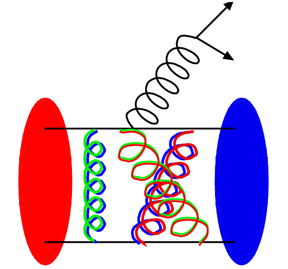


Neutral kaon mixing is an important process through which we can study CP violation in that system. In the Standard Model it proceeds via the ‘box’ diagram shown in Figure 10 with boson exchange. On the lattice, we are working at relatively low energy scales compared to the boson mass and the version of the box diagram that is appropriate is that of a 4-quark operator from the effective weak Hamiltonian at low energy scales. The matrix element of this operator between neutral kaon states is parameterised by where is the decay constant and , the amount by which the matrix element differs from is known as the bag factor. An evaluation of the 4-q operator matrix element in lattice QCD along with experimental results for the direct CP violation ratio of decay rates of and , , allows a constraint on the CKM elements that enter the operator from and quarks appearing in the box diagram [30]. There is no need in principle to separate the matrix element into its and components, but this is usually done and the two numbers quoted separately. on its own is a relatively simple calculation, as described above, and has been calculated accurately in lattice QCD by several groups. The 4-q operator is a harder calculation and is complicated to renormalise in formalisms that do not have the complete continuum chiral symmetry. This has made it a good calculation for the domain wall quark formalism.

RBC/UKQCD have given a result for using domain wall quarks this year on their configurations including , , and sea quarks. They have calculations on both and lattices at a single lattice spacing of 0.11fm. They obtain where the first error is statistical and the second systematic [6]. However, their result for on the same lattices is currently 5% low. Encouraging preliminary results, but no final numbers, were also presented this year from a mixed-action approach using domain wall valence quarks on the MILC gluon configurations that include sea quarks with the improved staggered formalism at multiple values of the lattice spacing [31]. Errors below 5% are clearly possible on from lattice calculations in the near future.
Charm physics provides a key test of lattice QCD calculations because, as described earlier, it is more sensitive to discretisation errors coming from the lattice QCD method than light quark physics. A new formalism called HISQ quarks [5] has shown this year that it is possible to treat charm quarks in essentially the same way as light quarks. This makes for a very fast method (because it is based on the fast staggered formalism, but working at larger quark masses it is even faster) with the added advantage of being able to make use of light quark chiral symmetry to give conserved currents for calculating decay rates that do not need renormalisation (and their associated systematic errors). This then gives errors at the few percent level [12].
One significant test of the formalism, and one that has not been available from previous lattice calculations, is that of the simultaneous determination of the spectrum of charmonium states and charm-light states with the same charm quark propagators. Of course, in QCD we know that there is only one charm quark with a given mass, but most approximations to QCD, such as potential models, find it impossible to handle both sets of states in the same approximation since their internal dynamics is very different. On the lattice it is also true that systematic errors are very different in the two systems, with charmonium states being more sensitive to discretisation errors, so that a very accurate discretisation is needed to be able to describe both successfully. With HISQ we have this and so the value that the charm quark mass needs to take is fixed to get the mass correct (this being the lowest-lying charmonium state and one whose mass is most accurately calculated on the lattice). The and masses are then non-trivial predictions given a mass from and an quark mass from . Very accurate results are obtained using valence HISQ quarks on the MILC ensembles, which agree with experiment with 6 MeV errors, see Figure 11. This level of accuracy requires an understanding of corrections to the meson masses in the real world from QED effects and the fact that the and masses are not the same. To be working at the level of precision where these effects have to be considered is very exciting.

The and decay constants can also be determined to an accuracy of 2% using exactly the same method as for and described above. The results are shown in Figure 12. The leptonic decay rates of and mesons have now been measured by experiment and, given a value for the appropriate CKM element from elsewhere, can be converted into a value for the decay constant that can be compared to lattice results. Figure 13 compares such experimental determinations of from BaBar, Belle and CLEO-c, using , with lattice results. The Fermilab/MILC collaboration lattice result is also shown. They use the clover formalism for charm quarks on the MILC ensembles and produced first results for and ahead of experimental results and with errors of 7% [32]. The value of shown in figure 13 is an updated one from this year’s lattice conference of 254(14) MeV [33]. The calculation of and in the clover formalism does require a renormalisation (and the error associated with this is included in the error estimate) and the mass of the charm quark in this case is fixed from the mass itself, so further independent checks of this calculation against other quantities need to be done. The two lattice calculations agree well although they use very different charm quark formalisms, albeit on the same gluon ensembles. Further work is underway from other groups using other formalisms and ensembles.
On this quantity the lattice results are ahead of experiment, although experimental errors are expected to improve by a factor of two over the coming year. The experimental central values will have to come down as that happens if there is to be agreement. One outstanding issue is that of electromagnetic effects in the experimental result since the decay constant is defined in pure QCD [34]. More work needs to be done in the and cases to ensure that is not an issue at the level of precision we are aiming for in this comparison between theory and experiment.


Neutral mesons can mix in an analogous way to mesons. In this case it is simpler, being dominated by a single box diagram with quarks in, and reducing to a 4-quark operator with coefficient (see Figure 10). The matrix element of this operator is parameterised by where is the decay constant. In the past there has been a lot more work on the decay constant than on the 4-quark operator. This year, however, two groups, the HPQCD collaboration and the Fermilab/MILC collaboration, presented new results for the ratio of the 4-quark operator matrix element for the to that of the [35]. The results are at a preliminary stage currently but will be improved significantly over the coming year. The ratio is more accurate than the individual numbers because we cannot escape a renormalisation (and its associated error) of the matrix elements in this case, but the renormalisation is the same for and . Previously the HPQCD collaboration gave a result for of 1.20(3) [36]. This year the Fermilab/MILC collaboration give their value for this ratio as 1.22(3) [33]. Our prejudice is that should be very similar to , and the aim is certainly to achieve the same level of error, or better. HPQCD have given a result for of 0.281(21) GeV [37], where a lot of this error comes from the renormalisation.
Exclusive semileptonic decay is an important route to determining the CKM elements and . This year the Fermilab/MILC collaboration have determined the appropriate form factor for the process , including the effect of sea quarks fully for the first time [42]. The rate of this decay at zero recoil is proprotional to the square of , where is the form factor for and relatively at rest. Figure 14 shows the Fermilab/MILC results for at three different values of the lattice spacing using the MILC gluon field configurations including the effect of sea quarks. From their results they determine where the first error is statistical and the second systematic. Using the HFAG experimental average [43], this leads to a value for of where the first error is from experiment and the second from the lattice.
can be extracted from the exclusive process. Here lattice results are still not very accurate because the important kinematic region is one in which the mesons are moving rather fast and this gives a very noisy signal on the lattice. Work is underway to ameliorate this [44]. A recent theoretical determination of using combined lattice results from HPQCD and Fermilab/MILC along with light-cone sum rules gives [45]. The issue of compatibility of this result with that from the inclusive decay is becoming an important one [46].
IV Conclusions
Lattice calculations including the full effect of , and sea quarks are in excellent shape. Calculations using improved staggered quarks continue to get better and new results are now appearing from other quark formalisms. There have been significant new results this year in strange and charm physics. I have concentrated on results relevant to CKM physics and have not mentioned many other areas of progress in lattice calculations. The reader is referred for those to the proceedings of this year’s lattice conference [2].
In Figure 15 I have collected recent lattice results into a set of constraints on the upper vertex of the standard unitarity triangle plot. The lattice inputs needed are , , , , and . It is important to use lattice results from the calculations including the full effect of , and sea quarks. Old results in the quenched approximation are not reliable enough for this. They have in any case now been superseded and should not be used.
In the next two years the lattice errors on these CKM constraints should halve. The robustness of our error estimates will be further tested against experiment using other gold-plated results. for and are good tests for and physics, for example. We have no free parameters when we do this and so it is a very stringent test. The era of precision lattice QCD calculations has really arrived.

Acknowledgements. I am grateful to the conference organisers for the opportunity to give this talk and to the following people for assistance in preparing it: Claude Bernard, Peter Boyle, Eduardo Follana, Elvira Gamiz, Andreas Jüttner, Andreas Kronfeld, Jack Laiho, Peter Lepage, Paul Mackenzie, Craig McNeile, Matthew Moulson, Gerrit Schierholz, Enno Scholz, Junko Shigemitsu, Jim Simone, Doug Toussaint, Carsten Urbach, Ruth van de Water and Kit Wong.
References
- [1] C. T. H. Davies et al, Fermilab, HPQCD, MILC, UKQCD collaborations, Phys. Rev. Lett.92:022001, 2004.
- [2] Proceedings of Lattice2007, Regensburg, July 2007, PoS LAT2007.
- [3] A recent textbook on Lattice QCD is: DeGrand and DeTar, Lattice methods for Quantum Chromodynamics, World Scientific, 2006.
- [4] A. Kronfeld, PoS LAT2007:016, 2007.
- [5] E. Follana et al, HPQCD, UKQCD collaborations, Phys. Rev. D75:054502, 2007.
- [6] P. A. Boyle, PoS LAT2007:005, 2007, arXiv:0710.5880 [hep-lat].
- [7] H. Matsufuru, PoS LAT2007:018, 2007.
- [8] C. Urbach, PoS LAT2007:022, 2007.
- [9] Y. Kuramashi, PoS LAT2007:017, 2007.
- [10] C. Bernard, et al, MILC collaboration, PoS LAT2007:090, 2007.
- [11] G. Colangelo et al, Nucl. Phys. B271:136, 2005.
- [12] E. Follana, C. T. H. Davies, G. P. Lepage and J. Shigemitsu, HPQCD and UKQCD collaborations, arXiv:0706:1726[hep-lat].
- [13] P. Boucaud et al, ETM collaboration, Phys. Lett. B650:304, 2007.
- [14] A. Jüttner, PoS LAT2007:014, 2007.
- [15] S. Beane et al, NPLQCD collaboration, Phys. Rev. D75:094501, 2007.
- [16] C. McNeile, PoS LAT2007:019, 2007.
- [17] P. Lepage et al, Phys. Rev. D46:4052, 1992.
- [18] A. X. El-Khadra, A. S. Kronfeld and P. B. Mackenzie, Phys. Rev. D55:3933, 1997.
- [19] A. Gray et al, HPQCD and UKQCD collaborations, Phys. Rev. D72:094507, 2005.
- [20] D. Toussaint et al, PoS LAT2007:137, 2007.
- [21] I. Allison et al, HPQCD, Fermilab and UKQCD collaborations, Phys. Rev. Lett. 94:172001, 2005.
- [22] S. Gottlieb et al, Fermilab and MILC collaborations, PoS LAT2005:203, 2006.
- [23] R. Sommer, Nucl. Phys. B411:839, 1994.
- [24] F. Ambrosino et al, KLOE collaboration, Phys. Lett. B632:76, 2006.
- [25] W. J. Marciano, Phys. Rev. Lett. 93:231803, 2004.
- [26] C. Aubin et al, MILC collaboration, Phys. Rev. D70:114501. 2004.
- [27] W. M. Yao et al, J. Phys. G33, 1 (2006).
- [28] P. A. Boyle et al, RBC and UKQCD collaborations, arXiv:0710.5136[hep-lat].
- [29] M. Moulson, private communication.
- [30] A. J. Buras, Les Houches 1997, hep-ph/9806471.
- [31] C. Aubin, J. Laiho and R.S. van de Water, PoS LAT2007:375, 2007.
- [32] C. Aubin et al, Fermilab, MILC and HPQCD collaborations, Phys. Rev. lett.95:122002, 2005.
- [33] J. Simone et al, Fermilab and MILC collaborations, PoS LAT2007:370, 2007.
- [34] W. J. Marciano and A. Sirlin, Phys. Rev. Lett. 71, 3629 (1993).
- [35] E. Gamiz et al, Fermilab and MILC collaborations, PoS LAT2007:354, 2007, C. T. H. Davies et al, HPQCD collaboration, PoS LAT2007:349, 2007.
- [36] A. Gray et al, HPQCD collaboration, Phys. Rev. Lett. 95:212001, 2005.
- [37] E. Dalgic et al, HPQCD collaboration, Phys. Rev. D76:011501, 2007.
- [38] M. Artuso et al, CLEO collaboration, Phys. Rev. Lett.99:071802, 2007; T. K. Pedlar et al, CLEO collaboration, Phys. Rev. D76:072002, 2007.
- [39] M. Artuso et al, CLEO collaboration, Phys. Rev. Lett. 95:251801, 2005.
- [40] B. Aubert et al, BaBar collaboration, Phys. Rev. Lett. 98:141801, 2007.
- [41] L. Widhalm, Belle collaboration, arXiv:0710.0420 [hep-ex].
- [42] J. Laiho, Fermilab and MILC collaborations, PoS LAT2007:358, 2007.
- [43] E. Barberio et al, HFAG, arXiv:0704.3575[hep-ex].
- [44] K. Y. Wong et al, PoS LAT2007:378, 2007.
- [45] J. M. Flynn and J. Nieves, Phys. Rev. D76:031302, 2007.
- [46] M. Neubert, these Proceedings.