Casimir scaling in G₂ lattice gauge theory

G₂ is the smallest of the 5 exceptional simple Lie groups, at the same time the simplest for which the universal covering group is the group itself, and both have a trivial center [15]. The basic information on the group can be found e.g. in [15, 17], a part is summarized here for the sake of completeness. The G₂ group has rank 2 and 14 generators. Its fundamental representation is 7-dimensional. G₂ is real and a subgroup of SO(7) of rank 3 with 21 generators, a group of $7\times 7$ orthogonal matrices $\mathbb{D}$ with unit determinant. G₂ matrices satisfy 7 additional cubic constraints:

where $T$ is an antisymmetric tensor non-zero elements of which are listed above (up to permutations of indices).

For a study of higher representations we will need tensor decompositions of various tensor products. Group theory provides the following relations:⁴⁴ 4 The decompositions were obtained using LiE, a clever computer algebra package for Lie group computations. For details, see [25].

Assume now $\mathbb{D}^{\{D\}}(g)$ is a matrix corresponding to an element $g\in{}$G₂ in its $D$-dimensional irreducible representation. Then the relations (9) imply that traces of higher-representation matrices can be expressed through traces of the fundamental- and adjoint-representation matrices:⁵⁵ 5 We suppressed the argument $g$ and used $F$ and $A$ instead of $\{7\}$ and $\{14\}$ to denote the fundamental and adjoint representation respectively. The symbol Tr is understood in the usual matrix sense, i.e. $\mbox{Tr}\;\mathbb{D}^{\{d\}}=\sum_{a=1}^{d}\mathbb{D}^{\{d\}}_{aa}$.^,66 6 A careful reader might notice that, in the case of SU(3), a well-known decomposition $\{3\}\otimes\{3\}=\{6\}\oplus\{\bar{3}\}$ leads to $\mbox{Tr}\;\mathbb{D}^{\{6\}}=(\mbox{Tr}\;\mathbb{D}^{F})^{2}-(\mbox{Tr}\;\mathbb{D}^{F})^{*}$, while Refs. [9, 10] used $\mbox{Tr}\;\mathbb{D}^{\{6\}}=\frac{1}{2}\left[(\mbox{Tr}\;\mathbb{D}^{F})^{2}+\mbox{Tr}\;(\mathbb{D}^{F})^{2}\right]$. Both formulas (and similar pairs for other representations of SU(3)) can be shown equivalent using the Cayley–Hamilton theorem.

The adjoint-representation matrix is constructed from the fundamental one:

The eigenvalue of the quadratic Casimir operator for the $D$-dimensional irreducible representation $\{D\}$ of the G₂ group can be computed from its Dynkin coefficients $[\lambda_{1},\lambda_{2}]$ (see e.g. [26]; we adopted the convention used in [25]). The dimension $D$ of a representation of G₂ with Dynkin coefficients $[\lambda_{1},\lambda_{2}]$ is given by [27]:

where $\ell_{1}=\frac{1}{3}(1+\lambda_{1})$, $\ell_{2}=\frac{1}{3}(4+\lambda_{1}+3\lambda_{2})$, and $\ell_{3}=\frac{1}{3}(5+2\lambda_{1}+3\lambda_{2})$, while the ratio of its quadratic Casimir operator to that of the fundamental representation is [27]:

Explicit values for the six lowest representations of G₂ are listed in Table 1.

We closely follow the lattice formulation of G₂ gauge theory outlined in [16]. On links of a space-time lattice, one puts matrices $U_{\mu}(x)$ from the fundamental ($\{7\}$) representation of G₂. Those are represented by $7\times 7$ complex matrices in a parametrization suggested by [28], which makes explicit the separation into the G₂/SU(3) coset group and the SU(3) subgroup.⁷⁷ 7 Another parametrization of G₂ matrices, via Euler angles [29] using real matrices, was described in Appendix B of Ref. [21]. (Details of the parametrization can be found in Pepe’s review [16].) Generators of the G₂ algebra corresponding to this parametrization are listed in Appendix A.⁸⁸ 8 We are grateful to Axel Maas for deriving explicit expressions.

We use the Wilson action:

where $P_{\nu\tau}(x)=U_{\nu}(x)\;U_{\tau}(x+\hat{\nu})\;U^{\dagger}_{\nu}(x+\hat{\tau})\;U^{\dagger}_{\tau}(x)$. Thermalized lattice configurations can be generated by a combination of pure-SU(3) Cabibbo–Marinari updates followed by random G₂ transformations, and overrelaxation sweeps, see [22] for a more detailed description.

In most cases we work on asymmetric lattices with different lattice spacings in time ($a_{t}$) and space ($a_{s}$) directions, therefore the action (14) contains a parameter $\xi_{0}$ called the bare anisotropy. To reproduce the usual classical gauge action in the naive continuum limit, the bare anisotropy has to be chosen as $\xi_{0}=a_{s}/a_{t}$. However, what we need to achieve is a certain fixed ratio of lattice spacings in space and time directions in physical units, $\xi=a_{s}^{\mathrm{phys}}/a_{t}^{\mathrm{phys}}$. The renormalized anisotropy $\xi$ is a function of $\xi_{0}$ and $\beta$ in the Wilson action (14), below we will discuss a nonperturbative determination of $\xi_{0}=f(\xi,\beta)$ to get a desired value of $\xi$ for a given coupling $\beta$. Before that, we will recall a few basic facts about the determination of the static potential from rectangular Wilson loops.

Let us start from a symmetric lattice with lattice spacing $a$. On a set of thermalized lattice configurations, we measure expectation values $W(r,t)$ of Wilson loops of spatial extent $\mathbf{r}=r\cdot a$ and a temporal separation $\mathbf{t}=t\cdot a$.⁹⁹ 9 Boldface symbols, $\mathbf{x},\mathbf{t},\dots$, denote variables with the dimension of length/time, $x,t,\dots$, are used for dimensionless quantities, i.e. $\mathbf{x},\mathbf{t},\dots$, divided by $a$, or $a_{s},a_{t}$ on an asymmetric lattice. For large time separations

The static potential

consists of two contributions: the true $\mathbf{r}$-dependent static potential due to the interaction of a color source and anti-source, and the self energy contribution (independent of $\mathbf{r}$) divergent in the continuum limit. Thus we can write

(Potentials with a hat are dimensionless.)

On an asymmetric lattice one can introduce three different potentials, defined as:

The Wilson loop $W_{ss}$ has both sides in spatial directions, while the second side of $W_{st}$ lies in the temporal direction (i.e. the one in which the lattice is discretized more densely).

One can argue for a simple relation between the interaction potentials [10, 30]:

Arguments for the usefulness of working on an asymmetric lattice have been clearly discussed e.g. in [10, 31]: a reduction of lattice artifacts, a certain hope to decrease errors due to the influence of the self energy $\widehat{V}^{\mathrm{self}}$, etc. The determination of static potentials at a fixed separation of sources relies on relations like (15) and requires to evaluate $W$ at as many $t$ values as possible. Our main motivation for using asymmetric lattices thus was to have more data points available in the physical $t$ window. We worked with lattices $L^{3}\times(2L)$, but wanted to keep the total physical length of the lattice in all directions the same, i.e. the renormalized anisotropy $\xi=a_{s}^{\mathrm{phys}}/a_{t}^{\mathrm{phys}}=2$. To determine the bare anisotropies $\xi_{0}=f(\xi,\beta)$ that lead to $\xi=2$ at the used values of the coupling $\beta$ we applied the procedure of [31]. One requires that the static potentials, which one can introduce on an asymmetric lattice, fulfill conditions (21) and (22). To avoid the nontrivial task of reliable determination of $\Delta\widehat{V}^{\mathrm{self}}$ in Eq. (21), we estimated $\xi_{0}$ using the latter condition.

In practice, we computed, for a given $\beta$ and lattice size, quantities:

and searched for a value of $\xi_{0}$ to fulfill

Of course, the obtained value of $\xi_{0}$ somewhat depends on the chosen pair of side lengths $(r,y)$ in Eq. (24). Since larger Wilson loops have smaller values and larger errors, we restricted ourselves to combinations $(2\div 3,2\div 3)$ only.

The described nonperturbative determination of $\xi_{0}$ was performed in simulations for $\beta=9.5$ (about 3000 configurations at each trial $\xi_{0}$) and $9.7$ (1000 configurations at each $\xi_{0}$) on a $12^{3}\times 24$ lattice. The results are summarized in Table 2. For production runs we chose values close to $\xi_{0}(2,3)$, but checked a rather weak dependence of results on its precise value. The value chosen for $\beta=9.6$ was obtained by linear interpolation.

Our final set of bare anisotropies used in production runs was $\xi_{0}=1.590,1.615,1.640$, for $\beta=9.5,9.6,9.7$, respectively.

Another problem of the determination of static potentials from Wilson loops is the insufficient overlap of the trial quark-antiquark state with the ground state, especially at larger spatial distances. An accepted remedy for this disease is not to construct Wilson loops directly from link matrices, but to use smeared links instead. Various variants of smearing have been proposed in the literature, we used the stout smearing procedure of Morningstar and Peardon [32]. The smearing is performed in several steps: First we calculate a weighted sum $S_{\mu}(x)$ of staples neighboring the link $U_{\mu}(x)$:

$\rho$ is a free parameter of smearing. We sum over directions $\nu$ depending on the potential studied (perpendicular to the Wilson loop, used for calculation of the potential). In the second step we project the product $\Omega_{\mu}(x)=S_{\mu}(x)U_{\mu}^{\dagger}(x)$ (no sum over $\mu$!) into the G₂ algebra using:

where $t_{a}$ are generators of the algebra (see Appendix A). In the last step, the smeared link is calculated as

The exponential function of matrices was calculated by means of spectral representation and LAPACK subroutines.

After an extensive exploration of the effect of the free parameter $\rho$ and of the number of smearing steps $N_{\mathrm{sm}}$ used on the ground-state overlap, we chose $\rho=0.1$. The optimal number of smearing steps was determined for each kind of potential: $N_{\mathrm{sm}}=20$ for $V_{st}$, $N_{\mathrm{sm}}=15$ for $V_{ss}$, and $N_{\mathrm{sm}}=5$ for $V_{ts}$ (see Appendix B for details). In production runs we always applied all three smearing procedures on each thermalized configuration separately, i.e. each time we smeared a new configuration using different staples and different number of smearing steps to get best overlap for a given potential.

As expected, smearing did enhance the ground-state overlaps considerably for all studied types of potentials. Not to overcrowd the main body of the paper with technicalities, some illustrative examples are supplied in Appendix B.

As discussed earlier (Sec. III.3), on an asymmetric lattice one can determine three kinds of potentials from the expectation values of Wilson loops of various orientations, $W_{\lambda}(r,t)$, where the index $\lambda$ assumes values $ss$, $st$, or $ts$. The corresponding potentials (in lattice units) can be determined [cf. Eq. (15)] by fitting logarithms of the measured loops by linear functions in $t$:

in an appropriate interval of $t$ values, from $t_{\mathrm{min}}$ to $t_{\mathrm{max}}$. Usually, to get a reasonable fit, one has to seek a compromise between two conflicting requirements: on one hand, to have a sufficiently long $t$-interval, i.e. to use as small $t_{\mathrm{min}}$ and as large $t_{\mathrm{max}}$ as possible, and, on the other hand, not to use too large $t$ values to avoid loops measured with unacceptably large error bars. In practice, however, with smeared links the problem turned out to be less severe: logarithms of Wilson loops were to a good approximation linear down to $t=1$ (see below), so we could choose for our fits $t_{\mathrm{min}}=1$. The upper limit $t_{\mathrm{max}}$ was chosen as a value, at which the quantity used to monitor the ground-state overlap (see Appendix B) dropped considerably or its error was of the size of its value.

A linear fit (28) in a fixed $(t_{\mathrm{min}},t_{\mathrm{max}})$-interval using the standard least-square method provides an expected value of $\widehat{V}_{\lambda}(r)$ together with an estimate of its statistical error, $\delta\widehat{V}_{\lambda}(r)$. This is almost certain to be an underestimate of the true error of the determination of the potential: there exists also a systematic error due to the unavoidably subjective nature of the choice of the fitting interval. To make at least a rough estimate of the order of magnitude of this systematic error, we used a kind of “jackknife-like” procedure: From the interval $(1,t_{\mathrm{max}})$ we omit in turn the 1-st, 2-nd, etc., $j$-th point and make a linear fit (28) to data points without the omitted point. In this way we obtain an ensemble of fit values for $\widehat{V}_{\lambda}(r)$, and estimate the systematic error of the procedure as the square root of the variance of this ensemble. It turns out that at small $r$ values the systematic error is of the order of the statistical one, but at large $r$ values it is often an order of magnitude larger.

Finally, if we want to compare potentials at different values of the coupling $\beta$, we need to fix the physical scale. Usually, lattice spacings $a_{s}$ are expressed in units of the Sommer scale $r_{0}$ defined via the relation [33]:

In lattice QCD, one uses for the Sommer scale a phenomenological value of $r_{0}=0.5$ fm, in the case of G₂ we leave this scale unfixed. In fact, for illustrative purposes it suffices to use approximate proportionality of $a_{s}(\beta)/r_{0}$ to $\sqrt{\widehat{\sigma}(\beta)}$, where $\widehat{\sigma}(\beta)$ is the string tension measured in lattice units (see Figs. 7 and 8 in Sec. IV.3). A small correction due to the Coulomb coupling constant does not change the picture qualitatively.

In this subsection we summarize selected results for potentials between static quarks and antiquarks from the fundamental representation, and the main purpose is to calibrate our procedure and compare with results of an earlier investigation [21]. Results for higher representations are deferred until Sec. IV.3.

Our simulations were performed at three values of the coupling $\beta$ on the weak coupling side of the crossover region observed in Ref. [17]. Parameters of the production runs are summarized in Table 3.

Fig. 1 clearly illustrates the fact that has been mentioned in Sec. IV.1: logarithms of Wilson loops computed from smeared links are almost perfect linear functions of $t$. The example shows $W_{st}(r,t)$ for a series of $t$ values at fixed $r$. The corresponding value of the potential was then obtained by a fit (28). The resulting potentials were then parametrized by the usual Coulomb plus linear form:

(A hat over a number again indicates that it is dimensionless lattice quantity, no hat is needed on $\alpha$.)

To compare with results in the existing literature, we computed $\alpha$ and $\widehat{\sigma}$ in runs on a symmetric, $14^{4}$ lattice. The result is summarized in Table 4. The values of the string tension are in reasonable agreement with those of Ref. [21], obtained on $12^{4}$ lattice. The slight discrepancy between $\alpha$ values can be attributed to different smearing procedures adopted. (Ref. [21] used a variant of the procedure of [34].) The purpose of smearing is to reduce ultraviolet noise in lattice configurations that mostly influences the self-energy and Coulombic parts of the static potential, and efficiency of various procedures differs in achieving this goal. At $\beta=9.7$ also string tensions seem not to be compatible within errors. However, both numbers are quoted with statistical errors only, and may in fact agree if finite-size effects and/or systematic errors are taken into account. To support this claim, we determined the string tension by our procedure also on $12^{4}$ lattice, and obtained a value of 0.109(2). Finally, using $t_{\mathrm{min}}=2$ instead of 1 in potential fits (cf. the discussion in Sec. IV.1), we went further down to $\widehat{\sigma}=0.105(2)$. It should be clear that though statistical errors on string tensions are as low as 2–3%, the actual error may be of the order of 10%.

Next we turn to asymmetric lattices and determine parameters of the three potentials (18), (19), and (20). Those are summarized in Table 5.¹⁰¹⁰ 10 We have some data on static potentials for the fundamental representation also from simulations on a $16^{3}\times 32$ lattice, albeit with lower statistics. The estimated string tensions agree with those quoted above, no strong finite-size effect was observed in this case. E.g., our preliminary values from the $16^{3}\times 32$ lattice are $\widehat{\sigma}_{st}=0.199(2),0.129(2),0.097(2)$ at $\beta=9.5,9.6,9.7$, respectively. When looking at these numbers, one should keep in mind that the errors quoted are just statistical. We did not attempt to estimate systematic errors, which were discussed in Sec. IV.1. The most reliable determination of parameters of the static potential comes from Wilson loops $W_{st}$ with the $t$-direction of the loop along the long lattice direction (in which the lattice is more finely discretized).

One can now verify the correctness of the chosen values for the bare anisotropy $\xi_{0}$ (cf. Table 2). On the basis of Eq. (21) one expects $\widehat{\sigma}_{ss}\approx 2\widehat{\sigma}_{st}$ and $\alpha_{ss}\approx 2\alpha_{st}$, which is satisfied to a surprising accuracy. From the numerical values of the string tensions one obtains the renormalized anisotropies $\xi=2.00(7),1.97(12),$ and $1.96(16)$ for $\beta=9.5,9.6$, and $9.7$, respectively. Similar relations should hold between ss and ts parameters [see Eq. (22)]. However, they are fulfilled with worse accuracy, because of systematic errors mentioned above. The available $t$ intervals for determination of these potentials are short, since the overlap with the ground state drops fast with $t$ at larger values of $r$ (see Fig. 11 in Appendix B).

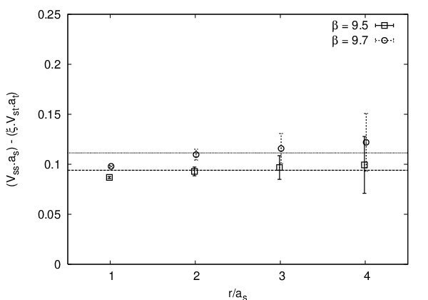
The fulfillment of relations (21) and (22) is visually displayed in Fig. 2 for $\beta=9.6$. The difference between $\widehat{V}_{ss}$ and $\xi\;\widehat{V}_{st}$ is expected to be a constant independent of $r$ (difference between self energies), our data support the expectation, see Fig. 3.

Finally, we checked that the exact value of the bare anisotropy $\xi_{0}$ is not of vital importance on asymmetric lattices. There were no large differences between the obtained potentials and their string tensions when we used $\xi_{0}=1.61$ instead of 1.59 at $\beta=9.5$, or $\xi_{0}=1.62$ instead of 1.64 at $\beta=9.7$.

After subjecting our procedure for determination of potentials to a number of tests in the case of the fundamental representation, we are ready to proceed to the main subject of the present paper: potentials between static color sources from higher representations of the G₂ group. For this purpose we will concentrate on potentials $\widehat{V}_{st}$ which can be determined most accurately. The procedure is now in principle straightforward. A thermalized configuration on an $L^{3}\times(2L)$ lattice is a set of link matrices in the fundamental representation. We smeared these links over “short” directions using the procedure described in Sec. III.5. Then, we compute a fundamental Wilson loop as a product of smeared link matrices along a closed loop (one side in a “short” direction, the other in the “long” one). Before taking a trace, we compute the matrix representing this loop in the adjoint representation using Eq. (11). Then we trace both the fundamental and adjoint Wilson loop matrix, and from these traces determine also those of the loop matrices in higher representations via the set of formulas (10). Finally, to obtain the expectation values of traces of Wilson loops of size ($r\times t$), we average over loop positions on a lattice, and over an ensemble of thermalized configurations in the usual way.

Illustrative results for Wilson loops in higher representations are displayed in Fig. 4 for $\beta=9.6$. The results look very much the same as in the case of the fundamental representation (Fig. 1). Values of the potential at various separations $r$ are obtained by fits of the form (28). The results for $\beta=9.6$ are shown in Fig. 5. It is clear that all higher potentials show a linear rise similar to the fundamental representation in the same range of distances.¹¹¹¹ 11 Though the string breaks in all representations of G₂, we had no ambition to observe it in our simulations. It is well known from earlier studies (see e.g. [35]) that it is of utmost difficulty to see string breaking on a lattice. Such a task is currently far beyond our possibilities, and is also not relevant to the main message of the paper.

The obtained potentials were fitted again by the Coulomb plus linear form (30). The resulting values of string tensions are summarized in Table 6. The measured values lie very close to predictions based on Casimir scaling, and the agreement with Casimir scaling tends to improve by increasing $\beta$, i.e. the deeper we enter the weak-coupling region above the crossover. In Fig. 6 this fact is exemplified on ratios of different representation potentials to the fundamental one at fixed $r$. At all distances, the ratios are close to the Casimir-scaling prediction, even though we made no attempt to get rid of the self-energy contributions.

In this context, the question of systematic errors again pops up: Could they not invalidate the above agreement with Casimir scaling? As discussed in detail in Sec. IV.1, the main source of the systematic error is the choice of the $t$-interval for linear fits of the form (28). To produce results in Table 6, $t_{\mathrm{min}}=1$ was used. The same analysis with $t_{\mathrm{min}}=2$ for the three lowest representations leads to values given in Table 7. The Casimir-scaling result comes out to be quite robust against this modification: though string tensions changed in all representations by up to 10%, they went in the same direction, and thus their ratios changed only slightly. In fact, at the largest available $\beta$, the agreement with Casimir-scaling prediction even improved.

Finally, we display the static potential for color charges in the fundamental (Fig. 7) and adjoint representation (Fig. 8) together for all three $\beta$ values, expressed in physical units defined by the fundamental string tension. All potentials nicely follow a universal curve.

References

- [1] J. P. Greensite, Nucl. Phys. B 158, 469 (1979); 166, 113 (1980).
- [2] P. Olesen, Nucl. Phys. B 200, 381 (1982).
- [3] J. Ambjørn, P. Olesen and C. Peterson, Nucl. Phys. B 240, 189 (1984); 240, 533 (1984).
- [4] L. Del Debbio, M. Faber, J. Greensite and Š. Olejník, Phys. Rev. D 53, 5891 (1996) [arXiv:hep-lat/9510028].
- [5] C. Michael, Nucl. Phys. B 259, 58 (1985).
- [6] C. Piccioni, Phys. Rev. D 73, 114509 (2006) [arXiv:hep-lat/0503021]; Casimir scaling in SU(2) lattice gauge theory, PhD Thesis, New York Univ., UMI–31–70864, 2005.
- [7] H. Markum and M. Faber, Phys. Lett. B 200, 343 (1988).
- [8] N. A. Campbell, I. H. Jorysz and C. Michael, Phys. Lett. B 167, 91 (1986).
- [9] S. Deldar, Phys. Rev. D 62, 034509 (2000) [arXiv:hep-lat/9911008]; Eur. Phys. J. C 47, 163 (2006) [arXiv:hep-lat/0607025].
- [10] G. S. Bali, Phys. Rev. D 62, 114503 (2000) [arXiv:hep-lat/0006022].
- [11] S. Gupta, K. Hübner and O. Kaczmarek, Phys. Rev. D 77, 034503 (2008) [arXiv:0711.2251 [hep-lat]].
- [12] J. Greensite, Prog. Part. Nucl. Phys. 51, 1 (2003) [arXiv:hep-lat/0301023].
- [13] M. Faber, J. Greensite and Š. Olejník, Phys. Rev. D 57, 2603 (1998) [arXiv:hep-lat/9710039].
- [14] M. Faber, J. Greensite and Š. Olejník, Acta Phys. Slov. 49, 177 (1999) [arXiv:hep-lat/9807008].
- [15] K. Holland, P. Minkowski, M. Pepe and U. J. Wiese, Nucl. Phys. B 668, 207 (2003) [arXiv:hep-lat/0302023].
- [16] M. Pepe, PoS LAT2005, 017 (2006) [Nucl. Phys. Proc. Suppl. 153, 207 (2006)] [arXiv:hep-lat/0510013].
- [17] M. Pepe and U. J. Wiese, Nucl. Phys. B 768, 21 (2007) [arXiv:hep-lat/0610076].
- [18] G. Cossu, M. D’Elia, A. Di Giacomo, C. Pica and B. Lucini, PoS LAT2006, 063 (2006) [arXiv:hep-lat/0609061].
- [19] G. Cossu, M. D’Elia, A. Di Giacomo, B. Lucini and C. Pica, J. High Energy Phys. 10, 100 (2007) [arXiv:0709.0669 [hep-lat]].
- [20] G. Cossu, M. D’Elia, A. Di Giacomo, B. Lucini and C. Pica, PoS LATTICE2007, 296 (2007) [arXiv:0710.0481 [hep-lat]].
- [21] J. Greensite, K. Langfeld, Š. Olejník, H. Reinhardt and T. Tok, Phys. Rev. D 75, 034501 (2007) [arXiv:hep-lat/0609050].
- [22] A. Maas and Š. Olejník, J. High Energy Phys. 02, 070 (2008) [arXiv:0711.1451 [hep-lat]].
- [23] J. Greensite and Š. Olejník, Phys. Rev. D 77, 065003 (2008) [arXiv:0707.2860 [hep-lat]].
- [24] J. Greensite and Š. Olejník, J. High Energy Phys. 09, 039 (2002) [arXiv:hep-lat/0209088].
- [25] M. A. A. van Leeuwen, Euromath Bull. 1, No. 2 (1994), http://www-math.univ-poitiers.fr/maavl/LiE.
- [26] R. N. Cahn, Semisimple Lie Algebras and Their Representations (Benjamin/Cummings, Menlo Park, CA, 1984).
- [27] M. J. Englefield and R. C. King, J. Phys. A: Math. Gen. 13, 2297 (1980).
- [28] A. J. Macfarlane, Int. J. Mod. Phys. A 17, 2595 (2002).
- [29] S. L. Cacciatori, B. L. Cerchiai, A. Della Vedova, G. Ortenzi and A. Scotti, J. Math. Phys. 46, 083512 (2005) [arXiv:hep-th/0503106].
- [30] J. Smit, Introduction to Quantum Fields on a Lattice: A Robust Mate, Cambridge Lect. Notes Phys. 15, 1 (2002).
- [31] T. R. Klassen, Nucl. Phys. B 533, 557 (1998) [arXiv:hep-lat/9803010].
- [32] C. Morningstar and M. J. Peardon, Phys. Rev. D 69, 054501 (2004) [arXiv:hep-lat/0311018].
- [33] R. Sommer, Nucl. Phys. B 411, 839 (1994) [arXiv:hep-lat/9310022].
- [34] K. Langfeld, Phys. Rev. D 69, 014503 (2004) [arXiv:hep-lat/0307030].
- [35] S. Kratochvila and P. de Forcrand, Nucl. Phys. B 671, 103 (2003) [arXiv:hep-lat/0306011].
- [36] L. Del Debbio, M. Faber, J. Giedt, J. Greensite and Š. Olejník, Phys. Rev. D 58, 094501 (1998) [arXiv:hep-lat/9801027].
- [37] G. S. Bali, K. Schilling and C. Schlichter, Phys. Rev. D 51 (1995) 5165 [arXiv:hep-lat/9409005].
- [38] S. Dürr, Comput. Phys. Commun. 172, 163 (2005) [arXiv:hep-lat/0409141].