Reinforced walks in two and three dimensions

Random walks with memory have a large number of applications in physics and other sciences. Many variants have thus been studied in different contexts. The best known example is presumably the self-avoiding walk [1], which models the large scale behavior of flexible chain polymers in good solvents. As pointed out by Amit et al. [2] the name ‘self-avoiding walk’ is something of a misnomer, since this model describes either static self-avoiding chains or self-killing walks. When the self-avoiding walker tries to revisit a site it has visited before, it is not gently turned towards another neighboring site; it is killed. In a more general version of this model, walkers carry an initial weight of unity, which decreases by a fixed factor whenever a site is revisited (the Domb-Joyce model [3]). If a site $i$ had been visited $n$ times before, the weight is diminished at the $n+1$ visit by $e^{nu}$ with $u<0$.

When the sign of the interaction is changed to $u>0$, so that the weight is multiplied by a factor $e^{nu}>1$ at each revisit, the resulting self-attracting walk degenerates in any finite dimension; for large times, the walker just oscillates between two sites. This extreme behavior is avoided if the weight change is independent of $n$ and one distinguishes only between sites which have and have not been visited before. This model is related to the Donsker-Varadhan [4] “Wiener sausage” problem [5] and leads to a power law scaling $R_{t}\sim t^{1/(d+2)}$ for the end-to-end distance after $t$ time steps in $d$ dimensions of space.

In contrast to these “static” models, where instances are weighted and the weights are modified by interactions, one can define “dynamic” models where the walks are biased by the interaction. The oldest such model is the true self-avoiding walk (TSAW) of Amit et al. [2]. Assume that at time $t$ the walker is at site $i$, and that the number of previous visits to any of the ${\cal N}$ neighbors is $n_{j},\;j=1,...,{\cal N}$. Then the probability to step to neighbor $j$ at the next time is

This is a much milder modification than the original self-avoiding walk. Accordingly, the r.m.s. end-to-end distance scales as $R^{2}_{t}\sim t$ for $d>2$, while there are logarithmic corrections at the ‘upper critical dimension’ $d=d_{c}=2$. In contrast, the upper critical dimension for the self-avoiding walk is $d_{c}=4$, and $R^{2}_{t}\sim t^{2\nu_{d}}$ for $d<d_{c}$ with $\nu_{d}<1/2$ [1].

When the sign of $u$ is switched to positive, the resulting “true self-attracting walks” (TSATWs) are also closer to random walks than the ordinary self-attracting walks. It seems that the behavior of the TSATW with $p_{j}$ given by Eq.(1) but with $u>0$ is unknown. On the other hand, there are several numerical studies of the TSATW with one-step reinforcement [6, 7, 8, 9, 10, 11]

where $\kappa_{j}=0$ if the site $j$ has never been visited before, and $\kappa_{j}=1$ otherwise. By far the most extensive studies were those of [10, 11], which claimed that one-step reinforcement TSATWs on the lattice showed a non-trivial phase transition in both $d=2$ and $d=3$, with $u_{c}(d=2)=0.88\pm 0.05$ and $u_{c}(d=3)=1.92\pm 0.03$. In both cases, the behavior of $R^{2}_{t}$ is supposed to change at $u_{c}$ from $R^{2}_{t}\sim t$ at $u<u_{c}$ to

at $u>u_{c}$. Hence the phase transition is between a random-walk-like and a collapsed phase. At the critical point, $R_{t}$ scales with a new exponent $\nu_{c}$ which is $0.40\pm 0.01$ in $d=2$ and $0.303\pm 0.005$ in $d=3$ [11]. These phase transitions are also seen in the average number $\langle S_{t}\rangle$ of sites visited up to time $t$. This scales as $\langle S_{t}\rangle\sim t$ for $u<u_{c}$ (with a logarithmic correction for $d=2$), but as $t^{k}$ with

for $u>u_{c}$. The latter was derived from a quasi-static approximation [12] in Ref. [6]. The quasi-static approximation seems to be satisfied to high precision (see below). At $u=u_{c}$, Ordemann et al. found $k_{c}=0.80\pm 0.01$ ($d=2$) resp. $0.91\pm 0.01$ ($d=3$) [11].

In a parallel and largely independent development, these and similar random walks with memory have been extensively studied in the probability theory literature. For a recent survey, see [13]. The rigorous mathematical study of reinforced walks displays much more breadth than the rather limited study of one-step site reinforcement in the statistical physics literature. In contrast to the physics literature, which focuses on the site model, bond or “edge” reinforced random walks (ERRW) have been studied in great detail and with multiple reinforcement as in Eq.(1) with positive $u$. Such walks (most clearly on trees) are closely related to Pólya urn processes and similar problems with reinforcement that can be solved exactly (note that walks with bond reinforcement are often called ‘trails’ in the physics literature [15]). For the models with multiple site reinforcement discussed above (called vertex-reinforced random walks or VRRW), the related urn process is Friedman-like and less tractable [13, 14], see endnote ¹¹ 1 We summarize the difference between these two urn processes following [14]. In the simplest Pólya urn, one begins with a single red and black ball. In a series of draws, one removes a ball at random and returns it to the urn with another of the same type. The fraction of red balls, surprisingly, converges to a random limit uniformly distributed on the closed interval $[0,1]$. In the Friedman urn, one reinforces both the drawn color and the other color. More surprisingly, the limit here converges to 1/2 even if the reinforcements are extremely biased towards the drawn color – as in [14] $1000$ to $1$ – although the convergence is extraordinarily slow..

The mathematicians have discovered profound differences between these two models. For example, ERRW is recurrent on finite graphs [16, 17], meaning that every edge is traversed infinitely often, while VRRW is not, becoming trapped e.g. on a line of five vertices [13, 14, 18] or more generally on “trapping subgraphs” [13, 14, 19, 20]. Many properties of the ERRW remain unknown; for example, the recurrence of ERRW on the infinite 2-d lattice is an open question. Even the one-step ERRW model (called once-reinforced in the mathematics literature) has only been successfully studied on a few special graphs, e.g. the infinite regular or Galton-Watson tree (where it is transient [13, 21, 22]) or the infinite ladder (where it is recurrent [13, 23]). The recurrence of one-step ERRW on the infinite 2-d lattice remains essentially open, although Sellke showed the separate recurrence of each coordinate [13, 24]. Pemantle [13, 14] provides a more complete description of these and other results.

The difference in mathematical tractability and underlying structure might suggest that models with bond and site reinforcement show different phenomenology. But this result would be unexpected from considerations of universality in statistical physics.

In the present paper, we clarify some of these issues by means of high precision simulations. Our main results are:

• •

  Bond and site reinforced TSATWs with one-step reinforcement show the same critical behavior and are likely in the same universality class;

• •

  There is no finite $u$ phase transition in the 2-dimensional TSATW model with one-step reinforcement. Walks are in the collapsed phase for all $u>0$ and the phase transition happens at $u_{c}=0$;

• •

  The critical point and the critical exponents for TSATWs with one-step reinforcement in $d=3$ are markedly different from the values obtained in [10, 11]; and

• •

  The quasistatic approximation for the end-to-end distance seems to become exact as $t\to\infty$ for the collapsed phase.

Simulations of TSATWs with one-step reinforcement are straightforward. To keep track of previous visits, one has to store a one-bit “spin” variable $s_{i}$ for each site (bond) $i$, and clear all spins after each walk. For convenience we sometimes used one byte per spin, which has the added advantage that clearing is needed only after every 255th walk. This requires $L^{d}/8$ resp. $L^{d}$ bytes of memory for site TSATWs and $dL^{d}/8$ resp $dL^{d}$ bytes for bond TSATWs. Memory limitations were more severe than CPU time so in the following we show more detailed results for site TSATWs than for bond TSATWs.

The most serious potential source of systematic errors arises from lattices that are too small. If open boundary conditions (b.c.) are used, the walk cannot go beyond the boundary, and both $R_{t}$ and $\langle S_{t}\rangle$ are underestimated. If periodic b.c. are used and the walk wraps around the lattice, it finds visited terrain in front of it and $R_{t}$ is overestimated, while $\langle S_{t}\rangle$ is still underestimated. We used lattices with helical boundary conditions and with up to $N=2^{32}$ sites ($d=2$) resp. $2^{34}$ sites ($d=3$), see endnote ²² 2 We always used lattice sizes such that the total number $N$ of sites was a power of two, in order to implement the boundary condition $i\equiv i-N\;\mod N$ by bit masking. The requirement that $N=L^{d}$ was not strictly enforced (unless $N$ was such that this would give an integer $L$), so the lattices were only approximately of cubic shape. This is of no consequence in the following.. For each walk, the spans $x_{\rm max}-x_{\rm min}$ in all $d$ directions were measured, and it was checked that the fraction of walks where any span was $\geq L$ did not exceed $10^{-4}$. This restricted the number of steps per walk to $t_{\rm max}\leq 10^{8}$ for $d=2$, and to $t_{\rm max}\approx 4\times 10^{7}$ for $d=3$. The total number of walks for each parameter setting was typically $\approx 2\times 10^{4}$ to $\approx 2\times 10^{5}$.

For small $u$, where walk-to-walk variation is significant, substantially increased accuracy is obtained by the following variance reduction procedure. Assume that the walker has already made $t$ steps and is presently at a site with cartesian coordinates ${\bf x}_{t}$. Given ${\bf x}_{t}$ and the states of the neighboring sites (i.e., visited or unvisited), one can calculate the expected increment $\widehat{\Delta\bf x}_{t+1}$ for the next step, since one knows the probability for the walker to step in each direction. From this, one obtains an estimate for the increment of $R_{t+1}^{2}$

where we have used the fact that $\widehat{\Delta\textbf{x}_{t+1}\cdot\Delta\textbf{x}_{t+1}}=1$. The improved estimate is obtained by summing these increments,

Further improvement is obtained by taking the optimal linear combination of the direct sample average and this estimator,

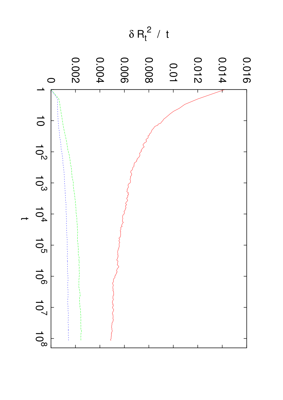
with $\alpha_{t}$ fixed for each $t$ such that the variance of $[R_{t}^{2}]_{\rm opt}$ is minimal. Differentiating the variance of $[R_{t}^{2}]_{\rm opt}$ with respect to $\alpha_{t}$ and minimizing this variance requires the estimation of the variances of $R_{t}^{2}$ and $\widehat{R_{t}^{2}}$ as well as their covariance. In Fig. 1 we show the errors (single standard deviations, divided by $t$) of the three estimators for 2-d site TSATWs with $u=0.34$.

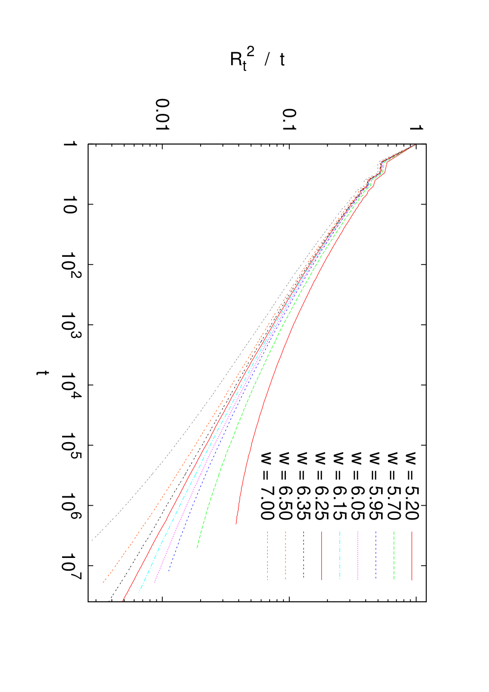
The average r.m.s end-to-end distance divided by the number of steps, $t^{-1}R_{t}^{2}$, is shown in Fig. 2 for site TSATWs in $d=3$. In this and in all subsequent figures, curves are not labelled by $u$ but by $w=\exp(u)$. We see clearly that there are significant corrections to scaling (all curves bend upward at small $t$), but they are no worse than in other nonequilibrium critical phenomena. A more careful analysis, taking these corrections into account, gives $u_{c}=1.831\pm 0.002$ ($w_{c}=\exp(u_{c})=6.24\pm 0.01$) and $\nu_{c}=0.378\pm 0.004$. In particular, we can rule out the possibility that $u_{c}>1.85$ from the simple fact that all curves for $u>1.85$ (i.e. for $w>6.35)$ are clearly S-shaped and curve down at large $t$. These estimates are incompatible with those of [11], $u_{c}=1.92\pm 0.03$ and $\nu_{c}=0.303\pm 0.005$. Possible explanations for these earlier results are that corrections to scaling were neglected in [11] or that the lattices used were too small.

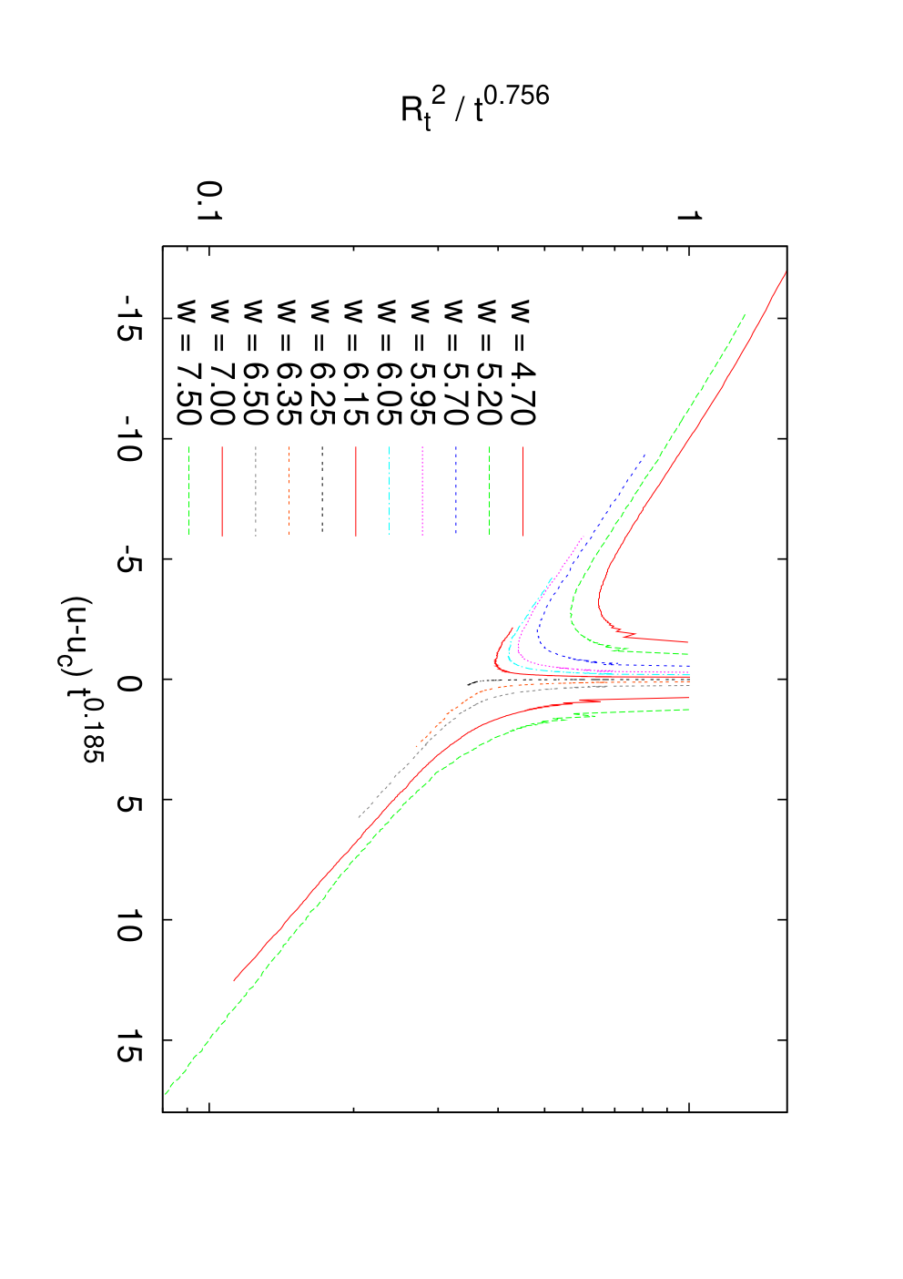
The cross-over behavior near $u\approx u_{c}$ can be fitted to the usual ansatz

with $\phi=0.185\pm 0.020$, as seen from the data collapse shown in Fig. 3. The deviations from a perfect collapse seen in this figure are due to the corrections to scaling at small $t$ seen in Fig. 2, which are not included in the scaling ansatz Eq. (8). The apparent collapse could have improved by the widespread practice of plotting the sub- and supercritical branches separately, without demanding that they join smoothly (the function $F(z)$ must be analytic at $z=0$). But the results obtained in this way would be spurious.

Results for the average number of visited sites, $\langle S_{t}\rangle$, again divided by $t$, are shown in Fig. 4. This time the corrections to scaling are much bigger. This is not unexpected, since there are also large corrections to the asymptotic law $\langle S_{t}\rangle\sim t$ for ordinary 3-d random walks. These corrections make an independent estimate of $u_{c}$ impossible, whence we shall use the estimate obtained from $R_{t}$, i.e. $u_{c}=1.831\pm 0.002$. The corrections to scaling also make the estimation of the exponent $k_{c}$ very uncertain, in spite of the extremely small statistical errors (much smaller than the thickness of the curves). Our best estimate is $k_{c}=0.977\pm 0.010$. This is again incompatible with the estimate $0.91\pm 0.01$ of [11]. The leading correction to scaling exponent, defined as $\langle S_{t}\rangle=t^{k_{c}}[a+b/t^{\Delta}+o(t^{-\Delta})]$, is found to be $\Delta=0.22\pm 0.03$. This is to be compared to $\Delta=1/2$ for ordinary 3-d walks [25].

For the supercritical case, $u>u_{c}$, the following argument was given in [6]: Let us assume that the visited sites form, for large $t$, a compact $d-$dimensional domain $V_{t}$ whose volume increases as $S_{t}\equiv|V_{t}|\propto R_{t}^{d}$ with $R_{t}\sim t^{\nu}$. Its surface is fuzzy but not fractal, i.e. it increases as $|\partial V_{t}|\propto R_{t}^{d-1}$. If the walker is uniformly distributed inside $V_{t}$, then the chance for it to be at the boundary is $|\partial V_{t}|/S_{t}\propto 1/R_{t}$. This is then also proportional to the chance that the walker will make the next step outside $V_{t}$, i.e. $d\langle S\rangle/dt\sim t^{-\nu}$. Integrating this gives $\nu=1/(d+1)$ [6]. The main assumption here is not that $\partial V_{t}$ is non-fractal (as stated in [6, 11]), but that the walker is uniformly distributed inside $V_{t}$. This would be exact if the boundary would not grow at all (i.e. in the limit $u\to\infty$), but for finite $u$ it corresponds to a quasistatic approximation in the sense of [12].

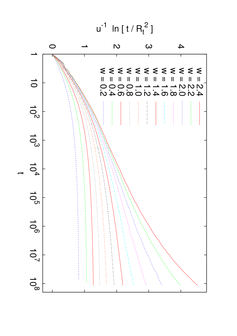
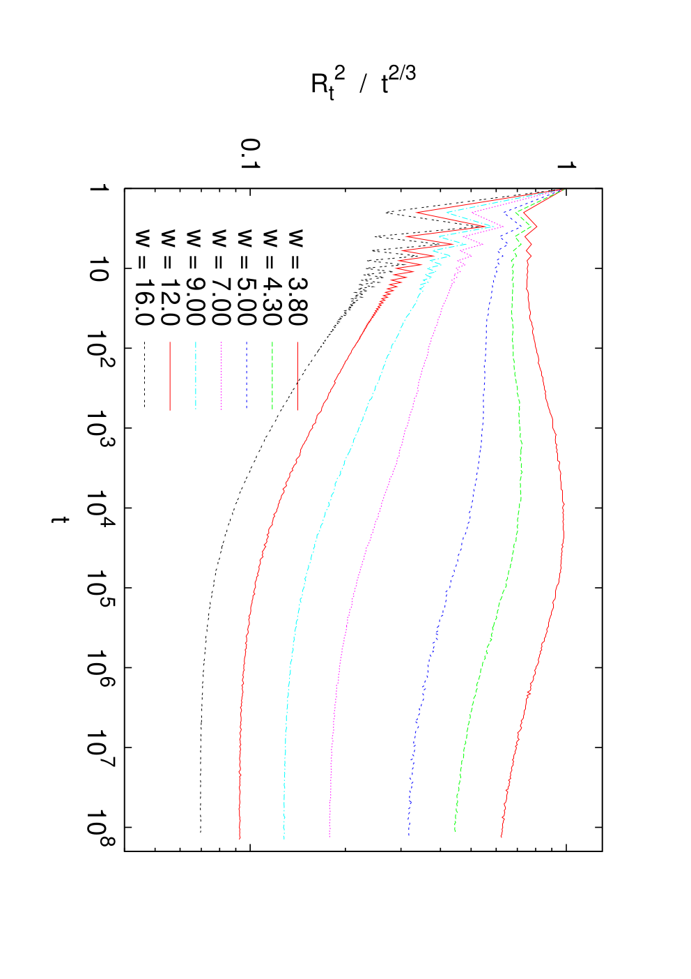
In order to test this quasistatic approximation of the supercritical behavior, we plot in Fig. 5 the ratio $R_{t}^{2}/\sqrt{t}$ for several values of $u>u_{c}$. We see very large corrections to scaling (the corrections to $\langle S_{t}\rangle$ would be even larger), but the curves do seem to become horizontal for $t\to\infty$. For $u\geq 2.5$, our best estimate is $R_{t}\sim t^{\nu}$ with $\nu=0.25\pm 0.01$, in perfect agreement with the prediction of the quasistatic approximation.

In two dimensions the situation seems at first glance similar, except for the fact that corrections to scaling are even larger. The latter is not surprising: random walks are recurrent in $d=2$, while they are not in any $d>2$. The number of visited sites increases not as $t$ in $d=2$, but as $S_{t}=\pi t/\ln(8t)[1+O(1/\ln t)]$ [25]. Related to this is the fact that true self avoiding walks have upper critical dimension $d=2$, leading to logarithmic corrections in most observables for $d=2$. As a consequence, one should also expect logarithmic corrections for TSATWs.

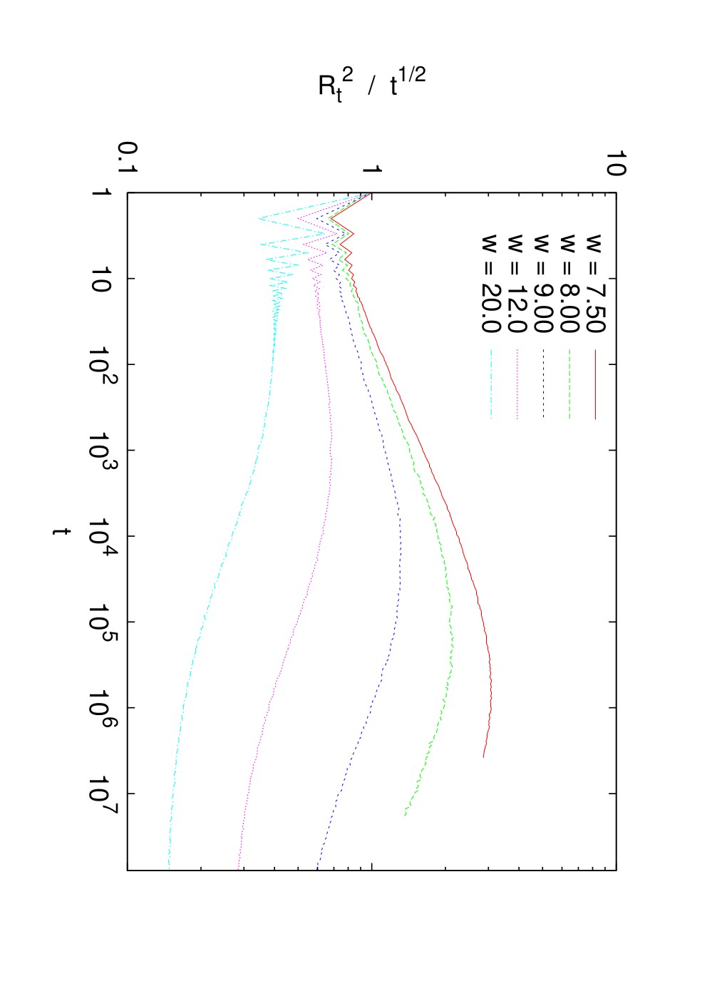
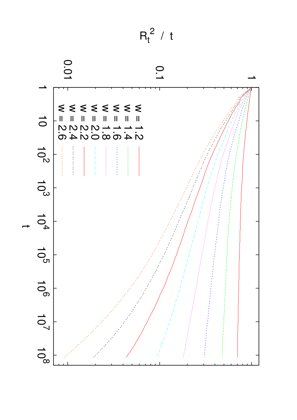
Results for the end-to-end distance are shown in Fig. 6. Again we show a log-log plot of $R_{t}^{2}/t$, for easy comparison with Fig. 2. The main difference between these two plots is that the curves fan out in Fig. 6 already for very small $t$, while they fan out only at much later times in Fig. 2. While the curves for $u<u_{c}$ in Fig. 2 first seem to follow the scaling $R_{t}\sim t^{\nu_{c}}$ and cross over to $R_{t}\sim t$ only at large $t$, no such cross-over is seen in Fig. 6. Careful inspection shows that all curves for $u>0.58$ (i.e. $e^{u}>1.79$) bend down at large $t$, indicating that $u_{c}\leq 0.58$ and that the estimate $u_{c}=0.88\pm 0.05$ of [11] is untenable. If we want to see a critical point with an associated non-trivial power law in these data, then a possible candidate is $u_{c}\approx 0.54$ and $\nu_{c}\approx 0.47$.

An attempted data collapse for the data of Fig. 6, again using Eq.(8) and optimized values $u_{c}=0.548,\nu_{c}=0.475$, and $\phi=0.085$, is shown in Fig. 7. We might mention that the exponents proposed in [11], $\nu_{c}=0.40\pm 0.01$ and $\phi\approx 0.2$, seem to be ruled out. A data collapse using these exponents is shown in panel (b) of Fig. 7. Although it has an acceptable overall dispersion, this is achieved mainly by fitting well the small-$t$ data, and grossly misrepresenting data for large $t$.

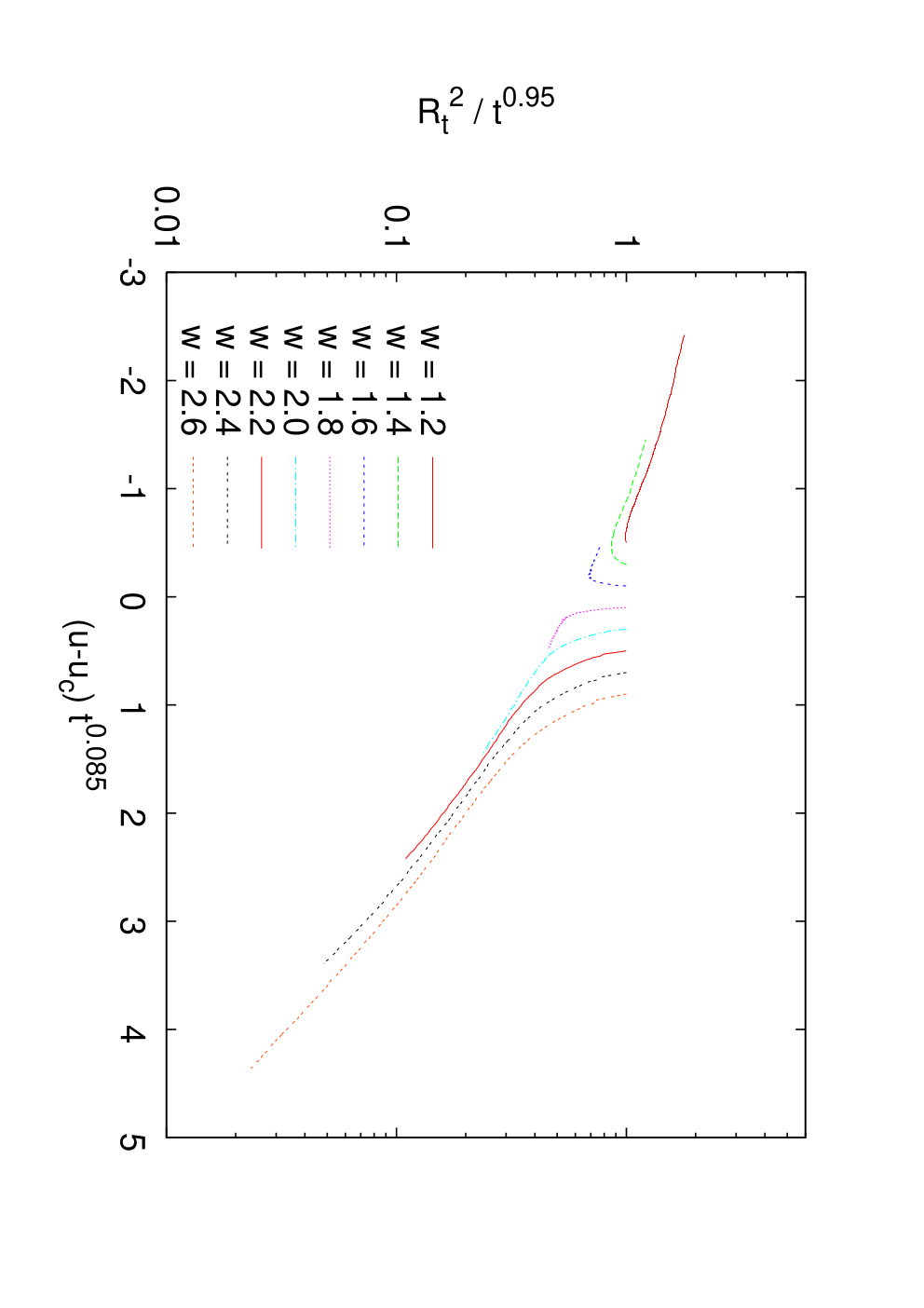
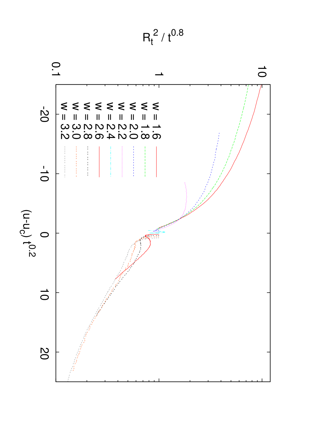
Although the collapse seen in Fig. 7(a) is satisfactory, the smallness of $\phi$ and the closeness of $\nu_{c}$ to the random walk value $\nu=1/2$ suggest a very different interpretation. We propose that there is in fact no phase transition at any $u_{c}>0$. Instead, the TSATW is collapsed for any $u>0$, i.e. $u_{c}=0$. This is also consistent with the fact that 2-d random walks are recurrent, i.e. the interaction should be a relevant perturbation for any $u>0$. It is difficult to obtain direct numerical evidence for this scenario, due to the very slow cross-over from the random walk behavior to the collapsed behavior, and due to the presence of strong corrections. In order to make any progress, we have to understand better these corrections.

In order to analyze the behaviour for very small $u$ more closely, let us define the quantity

It is obviously well defined for $u\neq 0$, but it can be defined also for $u=0$ using l’Hôpital’s rule,

We used here the fact that $R_{t}^{2}=t$ exactly for $u=0$. Numerically, $\Psi_{t}(0)$ can be estimated by a slight generalization of the reduced variance method discussed in subsection II.2. We simulate just ordinary random walks, but keeping track of the visited sites and calculating $\partial R_{t}^{2}/\partial u$ using Eqs. (2), (5), and (6).

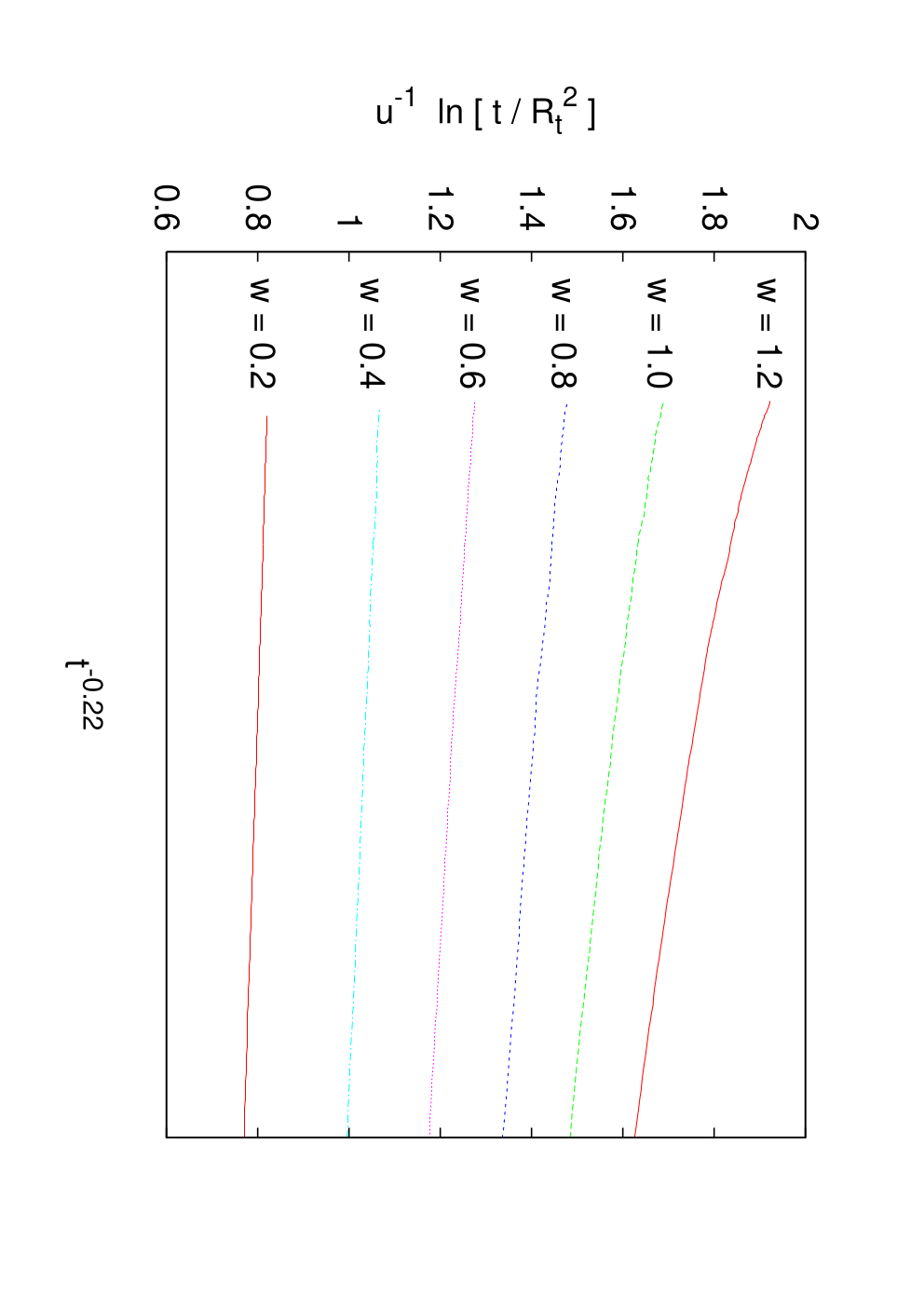
It is easily seen that $\Psi_{t}(u)$ is positive for all $u$. Plots of $\Psi_{t}(u)$ versus $t$, both for positive and for negative values of $u$, are shown in Fig. 8. Assume there is a collapse transition at $u=u_{c}$. We then expect that $\Psi_{t}(u)$ diverges as $\ln t$ for $u>u_{c}$ and $t\to\infty$, while it should stay bounded for $u<u_{c}$. More precisely, we expect that $\Psi_{t}(u)\sim const-a/t^{\delta}$ for $u<u_{c}$, where $\delta$ is another correction to scaling exponent. Plotting $\Psi_{t}(u)$ versus $t^{-\delta}$ should thus give straight lines converging to finite values for $t^{-\delta}\to 0$ if $u<u_{c}$, but upward bent curves diverging for $t^{-\delta}\to 0$ if $u>u_{c}$. One such plot, showing $\Psi_{t}(u)$ versus $t^{-0.22}$, is given in Fig. 9. From this and similar plots with different exponents, we conclude that (i) the data are consistent with this scenario; (ii) the critical point is at $u_{c}\approx 0$, most likely at $u_{c}=0$ exactly; (iii) the correction to scaling exponent is $\delta=0.22\pm 0.05$; and (iv) at the critical point, $\Psi_{t}$ scales either as $\Psi_{t}(0)\sim\ln\ln t$ or $\Psi_{t}(0)\sim[\ln t]^{\alpha}$ with $0<\alpha\ll 1$. The former ($\Psi_{t}(0)\sim\ln\ln t$) seems preferred, but a clear distinction between these alternatives is not possible.

Studying $S_{t}$, the number of visited sites, is not very revealing. As seen from Fig. 10, there is no value of $u$ for which the curve is straight. $u\approx 0.7,\;w=e^{u}\approx 2$ yields the straightest curve in the large $t$ range $10^{5}<t<10^{8}$, but this is clearly not asymptotic, as the curves for larger $u$ indicate (they have not crossed over to asymptotic behavior and hence curve up for large $t$, although they finally curve down, for very large $t$).

For coupling constants $u\gg 1$ one finds again that the prediction of the quasistatic approximation, $R_{t}\sim t^{1/3}$, is in excellent agreement with the data (see Fig. 11). As in the 3-d case, corrections to this prediction are very large for small values of $u$, but they decrease quickly for $u\to\infty$. One would like of course to verify the quasistatic approximation for smaller $u$, but this seems at present impossible without going to lattice sizes beyond the reach of our normal computational resources.

We now turn to the bond reinforced random walk in $d=3$. Results for the end-to-end distance $R_{t}^{2}$ are shown in Fig. 12. The plot is superficially quite similar to Fig. 2, with substantial corrections to scaling and the critical reinforcement $u_{c}$ occurring at much higher $u$. This latter fact is unsurprising as bond-reinforcement is much more “dilute” than its site-reinforced cousin; consider that the equivalent of a visited site in the bond-reinforced model must have all six bonds visited in $d=3$. Analysis suggests $u_{c}=2.475\pm 0.003$ and $\nu_{c}=0.380\pm 0.004$. Note that $\nu_{c}$ is within error of the estimate $\nu_{c}=0.378\pm 0.004$ for the Site TSATW in $d=3$. This is the first piece of evidence that the bond and site models are in the same universality class.

In Fig. 13 we show a data collapse with the same scaling ansatz Eq.(8); $u_{c}=2.475,\nu_{c}=0.380$ and $\phi=0.185\pm 0.020$. The critical exponents $\nu_{c}$ and $\phi$ are within error and identical, resp., to those for the Site TSATW in $d=3$, see Fig. 3, and the data collapse is if anything even better than that of Fig. 3. We see similar corrections to scaling at small $t$ and excellent collapse at large $t$, facilitated by our ability to simulate long walks ( $10^{7}$) due to the high value of $u_{c}$.

Results for the average number of visited sites, $\langle S_{t}\rangle$ are not shown, but are similar to Fig. 4, with substantial corrections to scaling. We thus use the estimate of $u_{c}$ obtained from $R_{t}$, i.e. $u_{c}=2.475\pm 0.002$. The best estimate of the exponent $k_{c}$ (again made difficult by corrections to scaling) is $k_{c}=0.970\pm 0.010$. This is incompatible with the estimate $0.91\pm 0.01$ of [11] but within the error of our estimate for the site-reinforced model, $k_{c}=0.977\pm 0.010$. The leading correction to scaling exponent, defined as $\langle S_{t}\rangle=t^{k_{c}}[a+b/t^{\Delta}+o(t^{-\Delta})]$, is found to be $\Delta=0.25\pm 0.05$. This is within error of the estimate $\Delta=0.22\pm 0.03$ in the site case.

Hence in all cases the estimates of the critical exponents for the site-reinforced model given by [11] are excluded by our results as candidate exponents for the bond-reinforced model. The estimates of all exponents for the bond-reinforced model agree (within error) with those we obtained for the site-reinforced case, see Sec. II.3. It is thus unsurprising that Fig. 14 similarly verifies the quasistatic approximation $R_{t}\sim t^{\nu}$ with $\nu=0.25$ for $u>u_{c}$ in the large $t$ limit. Crossover to the asymptotic behavior occurs at smaller $t$ as $u\to\infty$. It is harder to verify the large $t$ limit for small $u>u_{c}$; we cannot run sufficiently long walks while limiting spurious self-intersection and hence reliably estimating $R_{t}$.

Our results for $d=3$ indicate that the bond- and site-reinforced models are in the same universality class. This implies that $u_{c}=0$ for bond TSATW in $d=2$. To test this, we study small $u$ walks, which will cross over to the collapsed behavior only for large values of $t$. This regime is even more difficult to study in the bond reinforced case, due to the dilute nature of the bond reinforcement. The simulations used are as large as possible ($2^{32}$ sites and walks of $\approx 10^{8}$ steps) but in many cases these walks just reach the beginning of what may be the scaling regime.

In Fig 15 we show results for the end-to-end distance $R_{t}^{2}/t$. As in the site-reinforced case for $d=2$, the curves fan out in Fig. 15 for small $t$, with no apparent cross-over of the sort seen in Fig. 6 or Fig. 12. An estimate of the critical reinforcement $u_{c}$ from these data is extremely difficult. An attempted data collapse for the data of Fig. 15, using the scaling ansatz Eq.(8) and optimized values $u_{c}=0.73,\nu_{c}=0.481$, and $\phi=0.058$, is shown in Fig. 16(a). While the data collapse acceptably for these values, the exponents proposed in [11], $u_{c}=0.88,\nu_{c}=0.40\pm 0.01$ and $\phi\approx 0.2$, can be ruled out, as a data collapse using these exponents is completely unsatisfactory, Fig. 16(b) .

As the estimated $\phi=0.058$ is even smaller than that obtained for the site-reinforced model in $d=2$ (where $\phi=0.085$) and as $\nu_{c}=0.481$ is very close to the random walk value $\nu=1/2$, we argue that there is no phase transition for $u_{c}>0$ in the bond-reinforced model, either. In particular, similar heuristic arguments about the recurrence of 2-d random walks suggest again that any non-zero reinforcement is a relevant perturbation. Hence we study again the function $\Psi_{t}(u)$ [Eq. (9)] for $u>0$, $u=0$, and $u<0$ (see Fig. 17). As for the site case (subsection II.4), plotting $\Psi_{t}(u)$ against $1/t^{\delta}$ with different exponents $\delta$ reveals the detailed asymptotic behavior. Such plots (not shown here) indicate that $u_{c}=0$, and that the correction to scaling exponent in the uncollapsed phase $u<u_{c}$ is $\delta=0.20\pm 0.05$, well within error of the estimated $\delta=0.22\pm 0.05$ of the site case.

As was the case for the site-reinforced model in $d=2$, it is not particularly illuminating to study the number of visited sites $S_{t}$. The corrections to scaling are even larger, and hence it is impossible to estimate the correct scaling exponent from these data.

For coupling constants $u\gg 0$ one finds that the prediction of the quasistatic approximation, $R_{t}\sim t^{1/3}$, is in excellent agreement with the data (see Fig. 18). Corrections to this prediction are very large for small values of $u$, but become irrelevant as $u\to\infty$, as is already apparent at $w=e^{u}=16$. Familiar limitations to accessible lattice size make the quasistatic approximation impossible to verify for smaller $u$, where crossover to the asymptotic behavior takes place at very large $t$. Settling the validity of the quasistatic approximation in the small $u$ regime will in all likelihood require the development and application of appropriate analytical methods.

References

- [1] P.-G. de Gennes, Scaling Cpts in Polymer Physics (Cornell University Press, Ithaca, 1979).
- [2] D. Amit, G. Parisi, and L. Peliti, Phys. Rev. B 27, 1635 (1983).
- [3] C. Domb and G.S. Joyce, J. Phys. C 5, 956 (1972).
- [4] M.D. Donsker and S.R.S Varadhan, Comm. Pure Appl. Math. 28, 525 (1975); 32, 721 (1979).
- [5] V. Mehra and P. Grassberger, Physica D 168, 244 (2002).
- [6] V.B. Sapozhnikov, J. Phys. A 27, L151 (1994); 27, 3935 (1998).
- [7] F.D.A. Aaroro Reis, J. Phys. A 28, 3851 (1995).
- [8] M.A. Prasad, D.P. Bhatta, and D. Arora, J. Phys. A 29, 3037 (1996).
- [9] J.W. Lee, J. Phys. A 31, 3929 (1998).
- [10] A. Ordemann, G. Berkolaiko, S. Havlin, and A. Bunde, Phys. Rev. E 61, R1005 (2000).
- [11] A. Ordemann, E. Tomer, G. Berkolaiko, S. Havlin, and A. Bunde, Phys. Rev. E 64, 046117 (2001).
- [12] A. Jiménez-Dalmaroni and H. Hinrichsen, Phys. Rev. E 68, 036103 (2003).
- [13] R. Pemantle, Probability Surveys 4, 1 (2007); arXiv:math.PR/0610076v2 (2007).
- [14] R. Pemantle, Random processes with reinforcement, http://citeseer.ist.psu.edu/617028.html. Preprint (2001).
- [15] A. Guttman, J. Phys. A 18, 567 (1985).
- [16] P. Diaconis, In J. Bernardo, M. de Groot, D. Lindley, and A. Smith, eds., Bayesian Statistics, pp. 111-125. (Oxford Univresity Press, Oxford, 1988).
- [17] M. Keane and S. Rolles, In Infinite Dimensional Stochastic Analysis volume 52 of Verhandelingen, Afdeling Natuurkunde. Eerste Reeks. Koninklijke Nederlandse Akademie van Wetenschappen, pp. 217-234. (R. Neth. Acad. Arts Sci., Amsterdam, 1999).
- [18] P. Tarrès, Ann. Probab. 32, 2650 (2004).
- [19] R. Pemantle and S. Volkov, Ann. Probab. 27, 1368 (1999).
- [20] S. Volkov, Ann. Probab. 29, 66 (2001).
- [21] R. Durrett, H. Kesten, and V. Limic, Prob. Thoer. Rel. Fields 122, 567 (2002).
- [22] J. Die, Statistics Probab. Lett. 73, 115 (2005).
- [23] T. Sellke, Elec. J. Prob. 11, 301 (2006).
- [24] T. Sellke, Reinforced random walks on the -dimensional lattice. Preprint (1994).
- [25] D.C. Torney, J. Stat. Phys. 44, 49 (1986).
- [26] S.E. Derkachov, J. Honkonen and A.N. Vasil’iev, J. Phys. A: Math. Gen. 23, 2479 (1990).
- [27] B. Davis, Ann. Probab. 24, 2007 (1996).