Computation of the string tension in three dimensional Yang-Mills theory using large reduction
Abstract:
We numerically compute the string tension in the large limit of three dimensional Yang-Mills theory using Wilson loops. Space-time loops are formed as products of smeared space-like links and unsmeared time-like links. We use continuum reduction and both unfolded and folded Wilson loops in the analysis.
Keywords:
1/N Expansion, Lattice Gauge Field Theories1 Introduction
The method of large continuum reduction [1, 2] for gauge theory allows for the calculation of the infinite volume, infinite limit of certain physical quantities using volumes reduced to a small physical size. Numerical estimates [1, 2] of the physical critical size above which continuum reduction holds indicate that this method can be used to produce practical results. The chiral condensate [3] and the pion decay constant[4] were calculated in the large limit in four dimensions using continuum reduction. In this paper, we show that the method can be extended beyond bulk quantities and that it also produces reliable results for quantities with space-time dependence such as the heavy quark potential, from which the string tension can be extracted.
A precise calculation of the string tension in three dimensional gauge theories has been performed with up to 8 on large lattices [5]. In this paper, we present a complementary calculation with on lattices using continuum reduction. The calculation of Ref. [5] used correlation functions of smeared Polyakov loops to extract the string tension. After extrapolating to and to the continuum, the result was
| (1) |
where is the gauge coupling. This has to be compared with the analytical calculation in [6], namely, . Although the two results are not in perfect agreement, the main observation is that the approximations used in the analytical calculation are very well motivated.
The string tension for as per the analytical calculation [6] is
| (2) |
and are the quadratic Casimirs in the adjoint and fundamental representation, respectively. The mass parameter naturally enters the analytical calculation, and the second factor arises from the Wilson loop operator in the fundamental representation.
The numerical computation in [5] shows that the agreement gets better as one gets closer to . Like the analytical result, the numerical result also shows a correction from that goes like , but the coefficient of is not the same for the numerical and the analytical computations.
Since the numerical and the analytical results are close to each other even for (less than ), we can use the analytical formula to get a feel for the finite corrections to the infinite result. Therefore, we expect the finite corrections to be smaller than the error in Eqn(1) if .
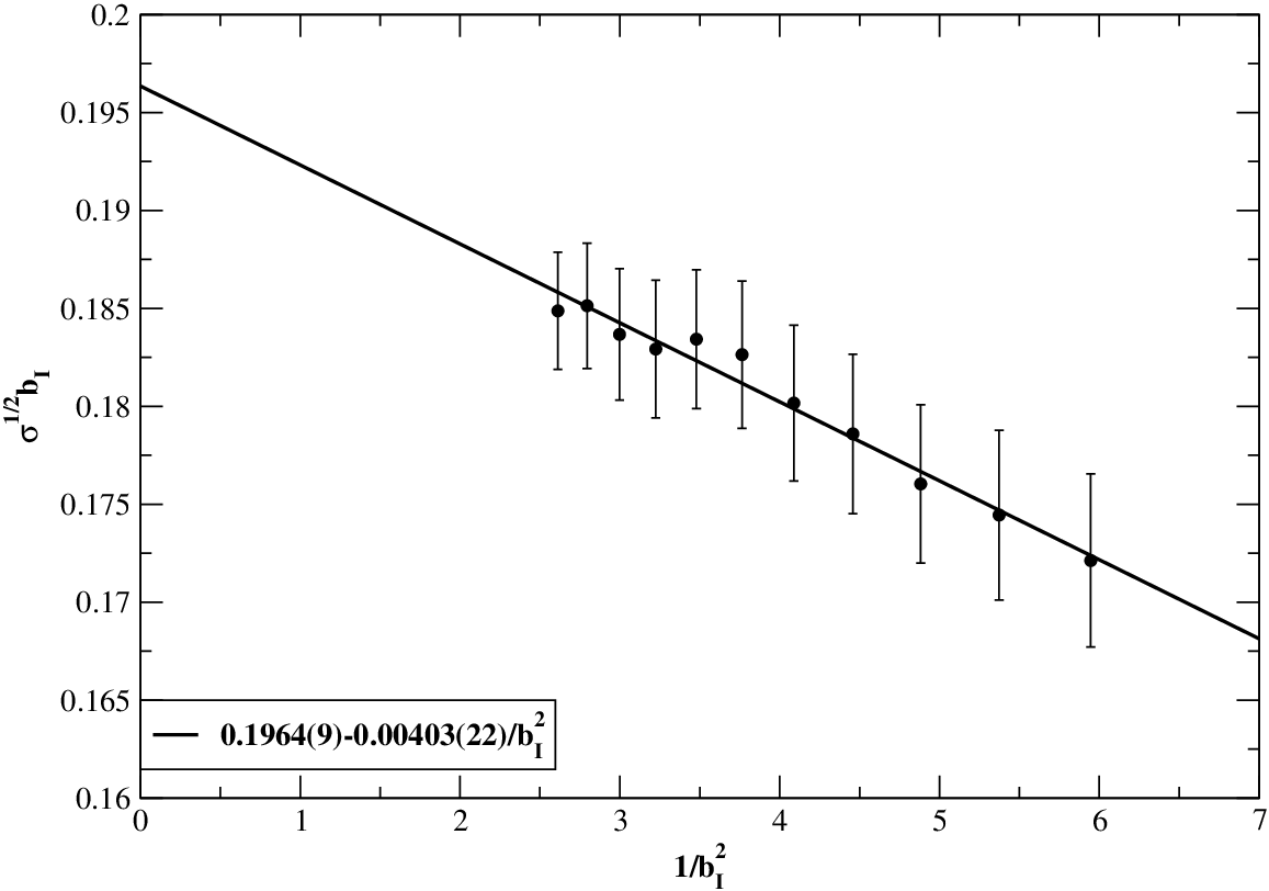
In this paper, we use continuum reduction [1, 2] to directly compute the limit of the string tension by working at large enough so that the finite corrections are smaller than the numerical errors. We find that
| (3) |
This result and that of (1) are consistent at the level of their one sigma errors. This level of agreement is, in turn, consistent with neither the large extrapolation of Ref. [5] nor the volume reduction of the present calculation having unexpected errors. While both of the numerical results lie below the analytical estimate, the discrepancy is relatively small. Thus the numerical evidence that the analytical result is an excellent first approximation that captures much of the physics remains strong.
The paper is organized as follows. We explain how we use smeared Wilson loops to compute the string tension in Section 2. The lattice results for the string tension along with the continuum extrapolation are also presented in this section. An intermediate step in our calculation is the dimensionless ground state string energy . In Section 3, we show results for at one fixed lattice coupling to illustrate its behavior as a function of and how it is used to extract the string tension. We also show that is unaffected by the smearing parameter. We illustrate the extraction of at one fixed coupling in Section 4. Here we show how the smearing parameter affects the overlap with the ground state. The main result in this paper is obtained using . We show that the finite and finite volume corrections are small at this value of in Section 5. We explain why this method is preferred over the Creutz ratio in Section 6.
2 String tension using Wilson loops and continuum reduction
Consider Yang-Mills theory on a periodic lattice with the standard Wilson gauge action. The method of [5] is to measure the string tension using correlations of Polyakov loops with separation that wind around a space direction. Continuum reduction [1, 2] implies that the large Yang-Mills theory in a continuum box of size is independent of as long as with being the deconfining temperature. One should be able to compute expectation values of Wilson loops of arbitrary size on an continuum box using folded Wilson loops and extract the string tension. To implement this approach to the three-dimensional Yang-Mills theory string tension, we use the following procedure:
- •
We fix the lattice size to . We use for the most part and only use to verify reduction.
- •
We fix so that finite corrections are small. We set and show using one instance that finite corrections are small at .
- •
We pick an appropriate range of lattice coupling .
- –
cannot be too small since we have to be away from the bulk transition on the lattice associated with the development of gap in the eigenvalue distribution of the plaquette operator [10]. Therefore, we pick .
- –
cannot be too big since we have to be below the deconfining transition for . Therefore, we pick [11].
- –
- •
We use smeared space-like links and unsmeared time-like links.
- •
We use the tadpole improved coupling to set the scale and consider Wilson loops with . This amounts to expectation values of Wilson loops that range from to .
- •
Keeping fixed, we fit
(4) where and are the dimensionless extent in the space and time direction respectively. is the dimensionless ground state energy. This fit assumes that there is a perfect overlap with the ground state. Note that should be zero since . Any small deviation from zero seen in the fit is due to the contribution from excited states. This can be seen by noting that should behave as with . Then, . The last term is numerically insignificant in the range of being considered.
- •
The use of smeared links improves the measurement of Wilson loops. They enhance the overlap of the space-like sides of the Wilson loops with the ground state. This increases the signal relative to the fluctuations and simplifies the behavior of the loops [7]. One step in the iteration takes one from a set to a set , by the following equation:
| (6) | |||||
| (9) | |||||
| (10) |
Note that time-like links, , are not smeared. Also note that smearing only involves space-like staples. There are two parameters, namely, the smearing factor and the number of smearing steps . Only the product matters, and plays the role of a discrete smearing step. For a given , the overlap of the smeared loop with the ground state does not depend on as long as it is small. But the overlap of the smeared loop with the ground state does depend upon . We set the value of the smearing parameter to by choosing and . To study the effect of varying , we also consider ( and ) at one coupling.
3 Extraction of string tension
gauge fields were generated on a periodic lattice using the standard Wilson action. One gauge field update of the whole lattice [2] is one Cabibbo-Marinari heat-bath update of the whole lattice followed by one over-relaxation update of the whole lattice. A total of such updates were used to achieve thermalization. Measurements were separated by such updates and all estimates are from a total of such measurements. Errors in all quantities at a fixed and were obtained by jackknife with single elimination.

The ground state energy obtained as a function of is fit to
| (11) |
We expect to approach a finite value in the continuum limit (). The same is expected for . For large, unsmeared or symmetrically smeared Wilson loops with , the universal value is [8] rather than the value for Polyakov loops [9] that was seen in [5]. The term is present due to the perimeter divergent contribution, and therefore it is expected to logarithmically diverge in the continuum limit. Since, we do not smear the time-like gauge fields, the divergence in this term is not tamed.
The method will encounter difficulties in extracting the physically relevant string tension from Eq.(11) if is large. However, because we do not go to very weak couplings, we see in Fig. 2 that is not too large. It is not necessary to go to weaker couplings since the string tension computed at the couplings we have chosen can be used to get a good estimate of the string tension in the continuum limit as is evident in Fig. 1.
The three parameter fit of as a function of is shown in Fig. 2. The fit has two degrees of freedom at the coarse lattice spacing of and has four degrees of freedom at the fine lattice spacing of . As mentioned before, errors in , , and are obtained by jackknife with single elimination. Unlike the estimate of the leading coefficient , the estimates of the sub-leading ones are not as reliable. Consider the dotted line and dot-dashed line in Figure 2. The constant term in each of these lines is obtained by evaluating at . The coefficient of the linear term in each is set to the same value as the one in the full three parameter fit. A comparison of the dotted line with the solid line and a comparison of the dot-dashed line with the dashed line shows that the term becomes relevant only if . There are only two data points at and three data points at where the effect is significant. As such, we do not expect our estimate of and to be as reliable as the estimate of .
The behaviors of and as a function of are shown in Fig. 4 and Fig. 4. Between these two terms, is the dominant one. The rise in at smaller is consistent with the presence of a term from a perimeter divergence. The estimate of is least reliable since it is dominated by the other two terms in the fit of as a function of . A fit of as shown in Fig. 4 is consistent with the existence of a continuum limit. One should note that the number of degrees of freedom in the three parameter fit of increases as decreases and this will have an effect in the determination of the sub-leading terms. We believe this is reason the fit of versus does not pass through all the data points. Since we do space-like but not time-like smearing and since our loops do not generally have , it not surprising to see a result that disagrees with the universal value but has the same sign and order of magnitude.
4 Extraction of


The dimensionless ground state energy is extracted at a fixed by fitting to as discussed in Sec. 2. While should be independent of the smearing parameter , the value of is expected to depend .
We will use as the coupling to illustrate the extraction of . Figure 6 and Fig. 6 show the performance of the fit for two different values of , namely, and respectively. The solid circles show the data points without errors. The solid lines show the fit of the data. Seven values of were used to fit the data at one , and data at seven different values of were fitted. This amounted to all Wilson loops from to on the lattice. The set of thermalized configurations used at is statistically independent from the set used at . The fit parameters are shown in Table 1 and Table 2. Only the average values of the fit parameters are listed.
Investigation of Table 1 and Table 2 shows that does not depend on . There is a small difference in the two values of at a fixed for the two different values of if is large. But Fig. 7 shows that this difference is within errors. Furthermore, the fitted values of for the two different values of are the same within errors.
| 1.62 | 3.23 | 4.85 | 6.47 | 8.08 | 9.70 | 11.31 | |
| 0.001 | 0.003 | 0.009 | 0.019 | 0.055 | 0.047 | 0.071 | |
| 0.133 | 0.218 | 0.286 | 0.347 | 0.399 | 0.464 | 0.517 |
The values of in Table 1 and Table 2 do show a variation with and . Since a smaller value of implies less smearing, the overlap with the ground state is less for smaller , and this results in a larger value of at smaller . The value of is very close to zero for small indicating excellent overlap with the ground state for the chosen value of . As increases, the length of the loop increases and the perimeter divergence has a stronger effect. This results in a larger value of as increases at a fixed .
| 1.62 | 3.23 | 4.85 | 6.47 | 8.08 | 9.70 | 11.31 | |
| 0.002 | 0.012 | 0.029 | 0.054 | 0.102 | 0.114 | 0.144 | |
| 0.133 | 0.218 | 0.287 | 0.349 | 0.404 | 0.468 | 0.526 |

5 Finite effects
Two issues need to be addressed with the analysis performed so far. We have fixed our value of assuming finite effects are small. If is not large enough, finite effects need to be addressed. In addition, we also have to address finite volume effects since continuum reduction is valid only in the limit.
We expect to have a fixed limit as at a fixed , , and . Indeed, this is the case as shown in Fig. 8 where the results for as a function of are shown for with on lattice. All three fit parameters are consistent within errors all the way from to . The only glitch one sees is at . This corresponds to , which is the linear extent of the lattice. One can argue that there are larger finite effects at strong coupling for . Since the fit of involves several values of , the larger effect at this particular value of is diminished in the extraction of .

Since finite effects can be ignored at , we also expect there to be no appreciable finite volume effects at this value of . This point is illustrated in Fig. 9 where the result for is plotted at and on and lattice. We used for this comparison since we have to be in the confined phase on lattice. Figure 9 shows that the two values of at a fixed are consistent with each other within errors. The same is the case for the fit parameter . This is not the case for and , and this is probably due to a three parameter fit using only five data points. Sub-leading coefficients are expected to depend sensitively on the data points. Since we are primarily concerned with the value of the string tension in this paper and since all our results are based on data taken on , we expect the final result to be free of finite and finite errors.

6 Creutz ratio
It is natural to ask how the Creutz ratio [12],
| (12) |
performs as an observable from which to extract the string tension. If we were to use Creutz ratios, we would have smeared all links using all staples. But one can still ask how the Creutz ratio behaves with the asymmetrically smeared links. We show this for square loops () at and in Fig. 10. The solid lines show the estimate for the as obtained from the analysis in this paper. There is no evidence for a plateau in the Creutz ratio in the range of shown in Fig. 10. It is possible the situation would be different if we had smeared all links.

Each data point in Fig. 10 is obtained using only four different Wilson loops, i.e. four of the data points in Fig. 6. This is quite different from the analysis in this paper. Seven different Wilson loops in Fig. 6 are used to extract one point in Fig. 2, and the loops used for different form independent sets. Then the are fit to determine the string tension. Both folded and unfolded loops contribute together. This is the main reason we succeeded in extracting the string tension using the range of Wilson loops considered here. To extract the string tension using Creutz ratios, larger loops and therefore larger statistics and possibly larger would be needed.
7 Conclusions
We used Wilson loops with smeared space-like links and unsmeared time-like links to obtain an estimate for the string tension in the large limit of three dimensional Yang-Mills theory. Invoking large continuum reduction, we included Wilson loops larger than the size of the lattice. Since we used smeared space-like links, the Wilson loops for fixed length in space and varying length in time showed excellent agreement with a single exponential. The ground state energy so obtained was fit using three parameters to get an estimate for the string tension. The ground state energy exhibited short distance behavior at the shortest length used in the paper but large enough distances were used to get an estimate for the dimensionless string tension with small errors (Equation 3). These results validate the method of continuum reduction for calculating quantities based on the space-time dependence Wilson loops.
Acknowledgments.
R.N. acknowledges partial support by the NSF under grant number PHY-055375.References
- [1] R. Narayanan and H. Neuberger, Phys. Rev. Lett. 91, 081601 (2003) [arXiv:hep-lat/0303023].
- [2] J. Kiskis, R. Narayanan and H. Neuberger, Phys. Lett. B 574, 65 (2003) [arXiv:hep-lat/0308033].
- [3] R. Narayanan and H. Neuberger, Nucl. Phys. B 696, 107 (2004) [arXiv:hep-lat/0405025].
- [4] R. Narayanan and H. Neuberger, Phys. Lett. B 616, 76 (2005) [arXiv:hep-lat/0503033].
- [5] B. Bringoltz and M. Teper, Phys. Lett. B 645, 383 (2007) [arXiv:hep-th/0611286].
- [6] D. Karabali, C. J. Kim and V. P. Nair, Phys. Lett. B 434, 103 (1998) [arXiv:hep-th/9804132].
- [7] M. J. Teper, Phys. Rev. D 59, 014512 (1999) [arXiv:hep-lat/9804008].
- [8] M. Luscher, K. Symanzik and P. Weisz, Nucl. Phys. B 173, 365 (1980).
- [9] P. de Forcrand, G. Schierholz, H. Schneider and M. Teper, Phys. Lett. B 160, 137 (1985).
- [10] F. Bursa and M. Teper, Phys. Rev. D 74, 125010 (2006) [arXiv:hep-th/0511081].
- [11] R. Narayanan, H. Neuberger and F. Reynoso, Phys. Lett. B 651, 246 (2007) [arXiv:0704.2591 [hep-lat]].
- [12] M. Creutz, Cambridge, UK: Univ. Pr. ( 1983) 169 P. ( Cambridge Monographs On Mathematical Physics)