Flow curves of colloidal dispersions close to the glass transition

The schematic $F_{12}^{\left(\dot{\gamma}\right)}$-model considers a single typical density correlator $\Phi\left(t\right)$ obeying a Zwanzig-Mori equation [24]:

$\Gamma^{-1}$ defines the (bare) time scale of the system. A vanishing memory kernel would lead to an exponential decay of the correlator. The equation of motion is closed by the self consistent approximation

and the normalization $\Phi\left(t\rightarrow 0\right)=1-\Gamma t$. Increasing the particle caging is modeled by increasing the coupling vertices $v_{i}\geq 0$. The parameter $\dot{\gamma}$ is the shear rate which leads to a strain dependent decay of the memory kernel. The parameter $\gamma_{c}$ is a scale for the magnitude of strain that is required in order for the accumulated strain $\dot{\gamma}t$ to matter [8].

For a vanishing shear rate, $\dot{\gamma}=0$, this model has been suggested by Götze [30] and describes the development of slow structural relaxation upon increasing the coupling vertices $v_{i}$. In this case the model shows two transition lines. For sufficiently small $v_{i}$ the nonergodicity parameter $f$ defined by the long time limit of $\Phi\left(t\right)$ is zero. By crossing one of the transition lines, $f$ becomes positive: $f=\Phi(t\to\infty)>0$. It is proved [31] that for a vanishing shear rate $\Phi\left(t\right)$ is completely monotone and $f$ is defined by the maximum real solution of $f+g\left(f-1\right)=0$ with $g=m(t\to\infty)=v_{1}f+v_{2}f^{2}$. This determines the transition lines. Vertices lying on a transition line and the corresponding nonergodicity parameters are denoted by $v_{i}^{c}$ and $f_{c}$. The type A transition line with $f_{c}=0$ is given by $v_{1}^{c}=1$, $0\leq v_{2}^{c}\leq 1$. By crossing this line $f$ varies continuously. The type B transition line, where $f$ jumps from zero to a finite value $f_{c}=1-\lambda$, can be parametrized by $\left(v_{1}^{c},v_{2}^{c}\right)=\left(\left(2\lambda-1\right),1\right)/\lambda^{2}$ with the exponent parameter $1/2\leq\lambda<1$. At $\left(v_{1}^{c},v_{2}^{c}\right)=\left(1,1\right)$ the type A transition line merges continuously into the type B transition line.

In the following we only consider vertices $v_{i}=v_{i}^{c}+\delta v_{i}$ close to the type B transition line. Then the dimensionless separation parameter measuring the distance from the transition point is defined by

With these definitions the model describes the dynamics of an ideal glass forming system. A negative value for $\varepsilon$ defines a liquid like state. For $\varepsilon\rightarrow 0^{-}$ an increasingly stretched plateau close to $f_{c}$ develops and the time scale for the final decay to zero depends sensitively on $\varepsilon$. A positive separation parameter leads to a glassy state where the nonergodicity parameter is determined to leading order by

A detailed discussion of the quiescent $F_{12}$-model can be found in [13].

For non-vanishing shear rates, $\dot{\gamma}\neq 0$, because of the vanishing long time limit of the memory kernel, also $f$ vanishes for all separation parameters. An arbitrary small but finite shear rate melts the glass and restores ergodicity. In the liquid state ($\varepsilon<0$), small shear rates have only little effect on the dynamics. But if the time scale for the shear induced decorrelation becomes faster than the time scale for the structural relaxation, then the long time dynamics is shear dominated and shows the same scaling behavior as for the glassy state ($\varepsilon>0$).

In the framework of the schematic model the steady state shear stress $\sigma=\dot{\gamma}\eta$, where $\eta$ denotes the viscosity, follows via integrating up the generalized shear modulus [10]:

The small negative quantity $0^{-}$ in Eq. (6) ensures that the integral in Eq. (5) includes the singularity of the $\delta$-function completely. The quantity $v_{\sigma}$ is assumed to be a constant and the parameter $\eta_{\infty}$ models viscous processes which require no structural relaxation [8]. The resulting linear moduli, the storage $G^{\prime}(\omega)$ and the loss modulus $G^{\prime\prime}(\omega)$, in the quiescent situation are discussed in Ref. [8]. We do not comment further on the Cox-Merz rule for which there is no basis in the asymptotic expansions of the $F_{12}^{(\dot{\gamma})}$-model.

We sketch some basic properties of the flow curves ($\sigma$ as a function of $\dot{\gamma}$). In the liquid state, because of the existence of $\eta_{0}=\int_{0}^{\infty}g\left(t,\dot{\gamma}=0\right)dt$, the flow curves show linear asymptotes for small shear rates and the yield stress $\sigma^{+}$, the zero shear limit of the stress $\sigma^{+}=\sigma\left(\dot{\gamma}\to 0\right)$, is zero. A simple Taylor expansion of $g\left(t,\dot{\gamma}\right)$ generalizes this statement: $\sigma=\dot{\gamma}\left(\eta_{0}+\eta_{\infty}\right)+\mathcal{O}\left(\dot{\gamma}^{3}\right)$. The Newtonian viscosity $\eta_{0}$ diverges at the glass transition according to the well known MCT power law, $\eta_{0}\propto\left|\varepsilon\right|^{-\gamma}$ [13]; see Eq. (18) below. In the glassy state, the time scale for the shear induced decay scales with $1/\left|\dot{\gamma}\right|$ which leads to a non vanishing yield stress. At $\varepsilon=0$ the yield stress jumps from zero to a finite value. For high shear rates, all flow curves converge to the common linear asymptote $\dot{\gamma}\left(v_{\sigma}/2\Gamma+\eta_{\infty}\right)$ where $v_{\sigma}/2\Gamma<\eta_{0}$. Hence the model describes the transition from a shear thinning liquid to a yielding glass [24]: In the liquid state, the viscosity starts at the plateau value $\eta_{0}+\eta_{\infty}$ for small shear rates and decays monotonically to a second plateau value $v_{\sigma}/2\Gamma+\eta_{\infty}$ for high shear rates. In the glassy state, the viscosity diverges in the zero shear limit.

The contribution of the parameter $\eta_{\infty}$ is only an additional constant to the viscosity which is not of interest for our work. Hence we choose $\eta_{\infty}=0$. In the following we choose for all numerical examples $v_{2}=v_{2}^{c}=2$ and $v_{1}=v_{1}^{c}+\varepsilon\left(1-f_{c}\right)/f_{c}$. For $\eta_{\infty}=0$ we easily verify:

Hence, without loss of generality, we choose units in such a way that $\gamma_{c}=\Gamma=v_{\sigma}=1$ and that $t$, $\dot{\gamma}$ and $\sigma$ are dimensionless. For the numerical solution of the $F_{12}^{\left(\dot{\gamma}\right)}$-model we use the algorithm first published in [32] with a grid size of $N=256$ and an initial step size of $h=10^{-6}$, see also [33] for details. All numerical parameters, which are relevant for our work, are tabulated in Appendix B.

For small separation parameters and shear rates the correlators develop a stretched dynamics located around the critical plateau value $f_{c}$. The discussion of the dynamics around this plateau, also called the $\beta$-relaxation process [13], is topic of this section. To derive the equation of motion to leading order in the separation parameter and the shear rate we first rewrite the convolution integral in Eq. (1) as $\int_{0}^{t}m\left(t-t^{\prime}\right)\dot{\Phi}\left(t^{\prime}\right)dt^{\prime}=\frac{d}{dt}\int_{0}^{t}m\left(t-t^{\prime}\right)\Phi\left(t^{\prime}\right)dt^{\prime}-m\left(t\right)$. Eq. (4) motivates the expansion

with $\mathcal{G}\left(t\right)=\mathcal{O}\left(|\varepsilon|^{1/2}\right)$. The function $\mathcal{G}\left(t\right)$ is often called $\beta$-correlator. By expanding the memory kernel in powers of $\dot{\gamma}$ and neglecting the time derivative we obtain to leading order the nonlinear stability equation [24],

with $c^{\left(\dot{\gamma}\right)}=\left(1-\lambda\right)/\lambda^{2}$. Eq. (10) has to be completed with the initial condition

where the exponent $a$ obeys

The time scale $t_{0}$ enables one to match Eq. (11) to the microscopic dynamics in the correlators. It has to be determined numerically by matching to the full solution for $\Phi(t)$ from Eq. (1). For $\varepsilon=0$ and $\dot{\gamma}=0$, the power law occurring in Eq. (11) is a special solution of Eq. (10) and describes the critical decay of $\Phi\left(t\right)$ to $f_{c}$ [13]. Fig. 1 shows representative examples.

One of the important aspects of $\mathcal{G}\left(t\right)$ are its homogeneity properties [24] which follow from Eq. (10). With some arbitrary scale $\Omega>0$ it obeys the two-parameter scaling law

with the master function obeying the initial condition $\hat{\mathcal{G}}\left(\hat{t}\rightarrow 0\right)=\left(\hat{t}\right)^{-a}$. Eq. (13) allows to define three regions. By choosing $\Omega=\left|\dot{\gamma}t_{0}\right|^{\frac{1}{1+a}}$ we obtain $\left|\hat{\dot{\gamma}}\right|=1$ and $\hat{\varepsilon}=\varepsilon/\varepsilon_{\dot{\gamma}}$ with the natural scale

The liquid region is defined by $\varepsilon\ll-\varepsilon_{\dot{\gamma}}$, where a finite shear rate barely distorts $\mathcal{G}\left(t\right)$. In the transition region, $\left|\varepsilon\right|\ll\varepsilon_{\dot{\gamma}}$, the dynamical anomalies are the most pronounced. The yielding glass region is defined by $\varepsilon\gg\varepsilon_{\dot{\gamma}}$. These definitions hold for $\left|\varepsilon\right|\ll 1$ and $\left|\dot{\gamma}t_{0}\right|\ll 1$ what we assume throughout in the following.

The present two-parameter scaling law bears some similarity to the one presented by Götze and Sjögren for the description of thermally activated processes in glasses [34]. In both cases, ideal glass states are destroyed by additional decay mechanisms. Yet, the ITT equations and the generalised MCT equations differ qualitatively in their description of the states at $\varepsilon\geq 0$. While the generalised MCT there predicts finite Newtonian viscosities, ITT predicts yield-stresses. Also both mechanisms can appear simultaneously and then need to be combined [8]. The similarity between both two-parameter scaling laws thus underlines the universality of the glass stability analysis, which is determined by quite fundamental principles. In Eq. (10), the shear rate can only be a relevant perturbation (at long times) if it appears multiplied by time itself. Symmetry dictates the appearance of $(\dot{\gamma}t)^{2}$, because the sign of the shear rate must not matter. The aspect that shear melts the glass determines the negative sign of $(\dot{\gamma}t)^{2}$.

Eq. (10) can be solved by using a generalized power series ansatz

where the exponents $u$, $\nu$ and the coefficients $\alpha$, $a_{1}$ obey

with $\Gamma_{n,n^{\prime}}=\frac{\Gamma\left(1+u+n\nu\right)\Gamma\left(1+u+n^{\prime}\nu\right)}{\Gamma\left(1+2u+\left(n+n^{\prime}\right)\nu\right)}-\lambda$ and the other coefficients are determined by the recursion formula $a_{n\geq 2}=-\frac{1}{2\Gamma_{0,n}}\sum_{n^{\prime}=1}^{n-1}\Gamma_{n-n^{\prime},n^{\prime}}a_{n-n^{\prime}}a_{n^{\prime}}$.

Along the lines of the work [34], we have analyzed all possible combinations that solve Eq. (16) in detail, see [33]. Each defines an (asymptotic) series expansion describing the dynamics in a special regime on a special time scale. There are four solutions for the liquid region, two for the transition region and three solutions describing yielding glassy dynamics. Here we only present a qualitative overview containing the leading asymptotes. In the liquid region, for short times $\mathcal{G}\left(t\right)$ follows $\left(t/t_{0}\right)^{-a}$ and merges into a second power law $-\left(t/\tau_{0}\right)^{b}$ for intermediate times with the von Schweidler exponent $b$ obeying

The two-parameter scaling law leads to

The parameter $\hat{\tau}_{0}$ has to be determined numerically. Without shear, the divergence of $\tau_{0}$ from Eq. (18) is the origin of the divergence of the Newtonian viscosity

where $G_{\infty}^{c}$ denotes the shear modulus (elastic constant) of the glass [8], and $\hat{\tau}_{\eta}$ is a constant. For long times $\mathcal{G}\left(t\right)$ merges into the linear asymptote $-t/\tau_{\dot{\gamma}}$ with

In the transition region, after following $\left(t/t_{0}\right)^{-a}$ the function $\mathcal{G}\left(t\right)$ merges into the long time asymptote $-t/\tau_{\dot{\gamma}}$. In the yielding glass region, $\mathcal{G}\left(t\right)$ follows $\left(t/t_{0}\right)^{-a}$, arrests on the plateau value $\sqrt{\varepsilon/\left(1-\lambda\right)}$ for intermediate times and merges into the linear asymptote $-t/\tau_{\dot{\gamma}}$ for long times. So we can summarize that the short- and long time asymptotes are common for all $\varepsilon$ if $\dot{\gamma}\neq 0$ is common. Fig. 2 shows an overview of the properties of $\mathcal{G}\left(t\right)$.

We briefly present the special asymptotic series expansion which is essential to understand the asymptotic behavior of the flow curves. For long times, $\varepsilon$ can be neglected on the left side of Eq. (16). We solve the resulting equation by choosing $u=1$ and $\Gamma_{0,1}=0$. The result can be written as

with $a_{1}^{*}=1$, $a_{n\geq 2}^{*}=-\frac{1}{2\Gamma_{0,n}}\sum_{n^{\prime}=1}^{n-1}\Gamma_{n-n^{\prime},n^{\prime}}a_{n-n^{\prime}}^{*}a_{n^{\prime}}^{*}$ and the exponent $c$ is defined by

A numerical example for $\varepsilon=0$ is shown in Fig. 2.

The coefficient $a_{1}$ has to be determined by matching to shorter time scales [24]. It obeys the two-parameter scaling law

Because of this scaling law, the non-trivial factor of ${a}_{1}$ depends on the ratio $\varepsilon/\varepsilon_{\dot{\gamma}}$ only:

This behavior will be crucial in the following as it enables us to describe the flow curves for small $\left|\varepsilon\right|$ and $\left|\dot{\gamma}t_{0}\right|$. Three limiting behaviors of ${a}_{1}$ can be determined, by identifying the time scales at shorter times, to which the series from Eq. (22) needs to be matched.

The results of the previous sections, especially Eq. (35) and Eq. (39), allow us to derive an analytical expression summarizing many aspects of the flow curves.

For sufficiently small $\varepsilon$ and $\left|\dot{\gamma}\right|$, because of the stretched dynamics, the dominant contribution to the integral in Eq. (5) is determined by the final decay of $\Phi^{2}\left(t\right)$ from the plateau to zero. Eq. (35) and Eq. (39) represent an asymptotic expansion for the shear-induced final decay of $\Phi\left(t\right)$. As demonstrated in Fig. 3, the first few low order terms are sufficient to describe the long time asymptote, provided that separation parameter and shear rate are sufficiently small. We notice that because of Eq. (40) and Eq. (41) the integrals

exist for $n\leq\left\lfloor 2/c\right\rfloor_{-}=3$ (here $\left\lfloor z\right\rfloor_{-}$ denotes the maximum integer number $n$ with $n<z$). Because of the rescaling of time in Eq. (30), the $\sigma_{n}^{*}$ are then constants. By taking only the integrable low order terms into account, we can write down an asymptotic formula for the shear stress:

Neglected higher order terms ${\cal O}\left(\left|a_{1}\right|^{\frac{2}{c}}\left|\dot{\gamma}\right|^{2}\right)$ are subdominant. Now we use the two-parameter scaling law for $a_{1}$ with the choice $\Omega=\left|\dot{\gamma}t_{0}\right|^{\frac{1}{1+a}}$ and define

for some arbitrary argument $x$. With the definitions $\sigma_{n}^{0}=\left(\hat{a}_{1}\left(0,1\right)\right)^{n}\sigma_{n}^{*}$,

we obtain the $\Lambda$-formula:

This is the central result of our work. Eq. (50) generalizes the results presented in [24] and [27] and summarizes many aspects of the flow curves.

Eq. (50) was obtained by integrating the correlators obeying the generalized ’time-shear-superposition principle’. Their amplitudes depend sensitively on shear rate and separation from the glass transition, as could be determined from the glass stability analysis. One function $\Lambda\left(\varepsilon/\varepsilon_{\dot{\gamma}}\right)=\hat{a}_{1}\left(\varepsilon/\varepsilon_{\dot{\gamma}},1\right)/\hat{a}_{1}\left(0,1\right)$ remained capturing this sensitive dependence, and in turn now determines the flow curves. In the following we discuss the properties of the $\Lambda$-formula in detail. General requirements for the range of validity are $\left|\varepsilon\right|\ll 1$ and $\left|\dot{\gamma}t_{0}\right|\ll 1$. The $\sigma_{n}^{0}$ are constants, which for our model numerically are obtained from fits.

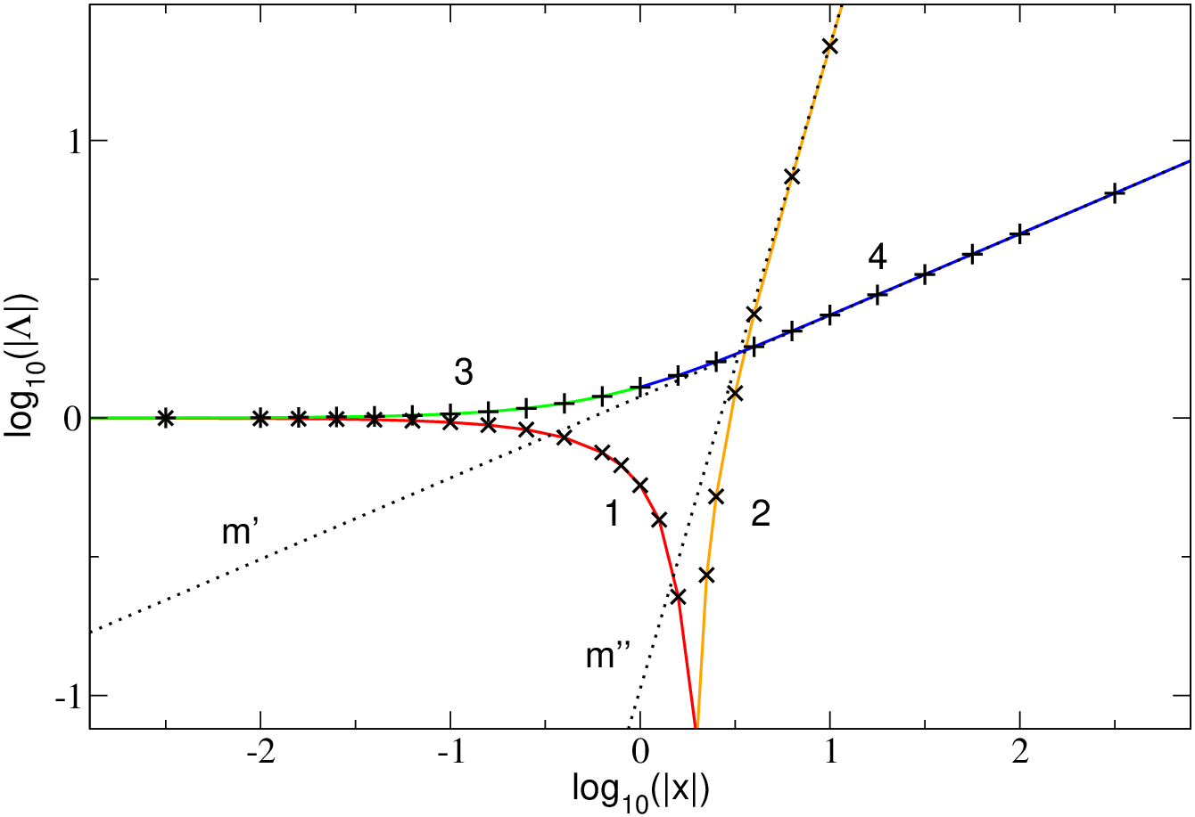
The central aspect of our work was to analyze the shape of $\Lambda\left(x\right)$ which we can determine numerically from $\mathcal{G}\left(t\right)$. This scalar function of one real parameter determines the shape of the flow curves within the range of validity of the $\Lambda$-formula. For instance, the asymptote for $x\rightarrow-\infty$ describes the flow curves in the liquid region while the asymptote for $x\rightarrow\infty$ describes the scaling of the yield stress for $\varepsilon>0$. We can determine three limiting behaviors.

By using Eq. (26), Eq. (27) and Eq. (28) we identify

We determine $\Lambda_{\infty}^{-}$ and $\Lambda_{\infty}^{+}$ numerically. Fig. 4 shows an overview of the properties of the $\Lambda$-function. A more detailed discussion can be found in Appendix A.

Fig. 5 shows an overview of the numerically obtained flow curves and the corresponding numerical results for the $\Lambda$-formula. While the glass flow curves exhibit an upward curvature only, the fluid curves show a characteristic S-shape, where the initial downward curvature changes to an upward one for increasing shear rate. For positive separation parameters the range of validity of the $\Lambda$-formula is given by $\left|\varepsilon\right|\ll 1$ and $\left|\dot{\gamma}t_{0}\right|\ll 1$. These two requirements ensure that $\mathcal{G}\left(t\right)$ describes the dynamics of $\Phi\left(t\right)$ with a sufficiently high accuracy. For sufficiently small negative separation parameters the $\Lambda$-formula is valid in finite shear rate windows only, as it does not reproduce the linear asymptotes for low shear rates. We find a precise criterion for the range of validity later when we discuss the limiting cases.

In the framework of the $\Lambda$-formula, it is easy to understand the mathematical structure of the singular behavior of the yield stress at $\varepsilon=0$: We choose some fixed $\varepsilon=\pm\left|\varepsilon\right|$ and consider the limit $\dot{\gamma}\rightarrow 0$. Then for $x=\varepsilon/\varepsilon_{\dot{\gamma}}$ we obtain $x\rightarrow\pm\infty$. The singular behavior is then due to the different asymptotes of $\Lambda\left(x\right)$ for $x\rightarrow\pm\infty$ while $\Lambda\left(x\right)$ itself is a smooth function for all $x$.

While Fig. 5 presents an overview of the flow curves, detailed discussions of the various limits are presented next.

References

- (1) W. B. Russel, D. A. Saville, and W. R. Schowalter, Colloidal Dispersions (Cambridge University Press, New York, 1989).
- (2) R. G. Larson, The Structure and Rheology of Complex Fluids (Oxford University Press, New York, 1999).
- (3) R. Besseling, Eric R. Weeks, A. B. Schofield and W. C. Poon, Phys. Rev. Lett. 99, 028301 (2007).
- (4) F. Varnik, L. Bocquet, and J. L. Barrat, J. Chem. Phys. 120, 2788 (2004).
- (5) F. Varnik and O. Henrich, Phys. Rev. B 73, 174209 (2006).
- (6) J. Bender and N. J. Wagner, J. Rheol. 40, 899 (1996).
- (7) R. Ganapathy and A. K. Sood, Phys. Rev. Lett. 96, 108301 (2006).
- (8) J. J. Crassous, M. Siebenbürger, M. Ballauf, M. Drechsler, D. Hajnal, O. Henrich and M. Fuchs, J. Chem. Phys. 128, 204902 (2008).
- (9) G. Petekidis, A. Moussaid, and P. N. Pusey, Phys. Rev. E 66, 051402 (2002); G. Petekidis, D. Vlassopoulos, and P. N. Pusey, Faraday Disc. 123, 287 (2003).
- (10) J. J. Crassous, M. Siebenbürger, M. Ballauf, M. Drechsler, O. Henrich and M. Fuchs, J. Chem. Phys. 125, 204906 (2006).
- (11) M. Fuchs and M. E. Cates, Phys. Rev. Lett. 89, 248304 (2002); M. Fuchs and M. E. Cates, in preparation (2007).
- (12) M. Fuchs and M. E. Cates, J. Phys.: Condens. Matter 17, S1681 (2005).
- (13) W. Götze, in Liquids, Freezing and Glass Transition, edited by J. P. Hansen, D. Levesque, and J. Zinn-Justin, Session LI (1989) of Les Houches Summer Schools of Theoretical Physics, (North-Holland, Amsterdam, 1991), 287.
- (14) W. Götze and L. Sjögren, Rep. Prog. Phys. 55, 241 (1992).
- (15) W. van Megen and S. M. Underwood, Phys. Rev. Lett. 70, 2766 (1993).
- (16) W. van Megen and S. M. Underwood, Phys. Rev. E 47, 248 (1993).
- (17) W. van Megen and S. Underwood, Phys. Rev. Lett. 72, 1773 (1994).
- (18) C. Beck, W. Härtl, and R. Hempelmann, J. Chem. Phys. 111, 8209 (1999).
- (19) E. Bartsch, T. Eckert, C. Pies, and H. Sillescu, J. Non-Cryst. Solids 307–310, 802 (2002).
- (20) T. Eckert and E. Bartsch, Faraday Discuss. 123, 51 (2003).
- (21) W. Götze, J. Phys.: Condens. Matter 11, A1 (1999).
- (22) J. M. Brader, Th. Voigtmann, M. E. Cates, and M. Fuchs, Phys. Rev. Lett. 98, 058301 (2007).
- (23) J. M. Brader, M. E. Cates, and M. Fuchs, in preparation (2008).
- (24) M. Fuchs and M. E. Cates, Faraday Disc. 123, 267 (2003).
- (25) M. Fuchs and M. Ballauff, J. Chem. Phys. 122, 094707 (2004).
- (26) M. Fuchs and M. E. Cates, J. Phys.: Condens. Matter 15, S401 (2003).
- (27) O. Henrich, F. Varnik and M. Fuchs, J. Phys.: Condens. Matter 17, S3625 (2005).
- (28) V. Carrier and G. Petekidis, J. Rheol., in print (2008).
- (29) D. Hajnal, O. Henrich, J. J. Crassous, M. Siebenbürger, M. Drechsler, M. Ballauf, and M. Fuchs, J. Rheol. submitted (2008).
- (30) W. Götze, Z. Phys. B 56, 139 (1984).
- (31) W. Götze and L. Sjögren, J. Math. Analysis and Appl. 195, 230 (1995).
- (32) M. Fuchs, W. Götze, I. Hofacker and A. Latz, J. Phys.: Condens. Matter 3, 5047 (1991).
- (33) D. Hajnal, Diploma Thesis, Universität Konstanz (2007). www.ub.uni-konstanz.de/kops/volltexte/2007/3800/ .
- (34) M. Fuchs, W. Götze, S. Hildebrand and A. Latz, J. Phys.: Condens. Matter 4, 7709 (1992).
- (35) M. Siebenbürger, D. Hajnal, O. Henrich, M. Fuchs, H. Winter, and M. Ballauf, in preparation (2008).