Cavity with an embedded polarized film: an adapted spectral approach
Abstract
We consider the modes of the electric field of a cavity where there is an embedded polarized dielectric film. The model consists in the Maxwell equations coupled to a Duffing oscillator for the film which we assume infinitely thin. We derive the normal modes of the system and show that they are orthogonal with a special scalar product which we introduce. These modes are well suited to describe the system even for a film of finite thickness. By acting on the film we demonstrate switching from one cavity mode to another. Since the system is linear, little energy is needed for this conversion. Moreover the amplitude equations describe very well this complex system under different perturbations (damping, forcing and nonlinearity) with very few modes. These results are very general and can be applied to different situations like for an atom in a cavity or a Josephson junction in a capacitor and this could be very useful for many nano-physics applications.
1) Laboratoire de Mathématiques, INSA de Rouen,
B.P. 8, 76131 Mont-Saint-Aignan cedex, France
E-mail: caputo@insa-rouen.fr
B.P. 8, 76131 Mont-Saint-Aignan cedex, France
E-mail: murkamars@hotmail.com
2) Department of Solid State Physics,
Moscow Engineering Physics Institute,
Kashirskoe sh. 31, Moscow, 115409 Russia
E-mail: amaimistov@hotmail.com
PACS: 42.60.Da Resonators, cavities, amplifiers, arrays, and rings, 77.55.+f Dielectric thin films
Keywords: Maxwell equations, mode conversion, cavity, recurrence
1 Introduction
There are many reasons to couple an oscillator to a cavity. One example is a laser built using a Fabry-Perot resonator enclosing an active medium which can be modeled as a two level atom [1, 2]. The cavity can also be used to synchonize oscillators [3] as for an array of Josephson junctions. For window Josephson junctions, used as microwave generators, the Josephson junction collects all the energy in one of the cavity modes [4]. The cavity can also be used as a thermostat to cool the oscillator as described in [5] where an optical cavity is used to cool an atom. In another example coupling an atom or quantum oscillator to a resonator can significantly change its transport properties [6].
In all the systems described above we have a localized oscillator coupled to a resonator. In addition the size of the oscillator can often be neglected. This situation can be represented by a thin film model [7, 8]. Such a thin film model was generalized by taking into account the local field effects (dipole-dipole interaction) [9, 10, 11]. Intrinsic optical bistability is the main result of this generalization. Thin films containing three-level atoms [12], two-photon resonant atoms [13, 14], inhomogeneously broadened two-level [15] atoms and two-level atoms with permanent dipole [16] represent the different generalizations of the model. The coherent responses of resonant atoms of a thin film to short optical pulse excitation were considered in [15]. It was shown that for a certain intensity the incident pulse generates sharp spikes in the transmitted radiation. Photon echo in the form of multiple responses to a double or triple pulse excitation was predicted also in this paper. The coherent reflection from a thin film as superradiation was studied in [18, 17, 19].
Recently we used the thin film model to describe switching phenomena in ferroelectrics [20]. The behavior of the new artificial materials – metamaterials – under action of electromagnetic pulses could be also described by this model [21]. As we see the thin film model is extremely fruitful, the investigation of the behavior of the thin film embedded inside the cavity is a very attractive problem. When the model of thin film is explored, the problem of the matter-field interaction reduces to the one of an electromagnetic cavity with an embedded (linear or nonlinear) oscillator. Frequently the nonlinear problem is analyzed using coupled mode equations. In this approach the relevant values are the amplitudes of each of the linear modes. The nonlinear partial differential equation of motion is reduced to a system of coupled ordinary differential equations for the amplitudes of the linear modes. A suitable choice of the linear modes allows to get an effective description of the original problem.
We consider here this simplest and most general situation, first for
small energy for which the problem is linear. In this case, the
system film/cavity has normal modes which we characterize. These
describe correctly the evolution of the system as opposed to
standard Fourier modes or even other simpler normal modes.
These adapted normal modes are
orthogonal with respect to an adapted scalar product. Using these
modes we can define simply the state of the system and obtain mode
conversion by acting on the film sub-system. In this paper we
propose the mode conversion mechanism for a linear system which can
be used for different applications. In the nonlinear case, for
medium amplitudes,
we show that a few modes are sufficient to describe the evolution of the system.
After introducing the model in section 2, we consider the linear limit in
section 3 and derive the normal modes of the system. The special
scalar product is derived in section 4. In sections 5 and 6 we use the
normal modes to define the state of the (linear) system and show
mode conversion when driving and damping the film. We also
describe the general nonlinear case and we conclude in section 7.
2 The thin film model
We consider a one dimensional model of the electromagnetic radiation interacting with a polarized dielectric film inside a cavity. The film is placed at the distance inside the cavity having the length . The Lagrangian density for the electromagnetic field, the film medium and their coupling is the following [20]:
| (1) |
Here is the analog of vector potential and is the medium polarization, is a coupling constant. The last term in Lagrangian describes the coupling between and . The dielectric medium can be ferroelectric () with two polarizations or paraelectric . The Hamiltonian of the system is
| (2) |
which gives
| (3) |
The variation of the action functional yields the Euler-Lagrange equations for and
| (4) |
| (5) |
which reduce to
| (6) | |||||
| (7) |
The equations for the electric field and medium variable can then be obtained
| (8) | |||||
| (9) |
where the coupling between the fields and only occurs in the medium at .
In a recent article [20], we considered with this model the interaction of a thin dielectric film with an electromagnetic pulse. We studied both the case of a ferroelectric and paraelectric film. For the ferroelectric film we showed that the polarization can be switched by an incoming pulse and studied this phenomenon. Here we will assume that the film is embedded in a cavity and we will study how cavity modes can be controlled by the film. Specifically we will assume Dirichlet boundary conditions for the field.
For small amplitudes of the field, it is natural to neglect the nonlinear response of the film. Note however that the ferroelectric film and paraelectric film have different natural frequencies corresponding to different stationary points. For the paraelectric case, there is only one fixed point while for the ferroelectric case there are three fixed points, the unstable one and the two stable ones corresponding to two opposite signs of the polarization. It is then natural to introduce the natural frequency of the oscillator for the paraelectric case and for the ferroelectric case. We therefore consider below the general linear problem of a harmonic oscillator of frequency embedded in a cavity.
3 The linear limit: normal modes
The linear problem is
| (10) | |||||
| (11) |
Note that we have a Dirac delta function in the first equation so that the solution will not have a second derivative at . In this case, one can write the solution using standard sine Fourier modes. However these are not adapted to describe the evolution because the projection of the operator gives wrong results [22]. Then we need to define new normal modes. For this one first separates time and space and one looks for solutions in the form
so that the system (10) becomes
| (12) |
As expected from the general theory of linear operators [23] the system will exhibit eigenfrequencies and eigenmodes (normal modes). Combining these two equations, we obtain the final boundary value problem for
| (13) |
with the boundary conditions .
To obtain the solution, notice that except for
Using this remark and the boundary conditions we get the left and right solutions
| (14) |
where and are constants. To connect the left and right solutions we use the continuity of as well as of at . The second relation needed is the jump condition for obtained by integrating (13) over a small interval centered on . When the size of the interval goes to zero we get
| (15) |
At the continuity of and jump condition (15) give the following relations
| (16) | |||
| (17) |
For this homogeneous system to have a non zero solution, the determinant must be zero and this gives the dispersion relation
| (18) |
which determines the allowed frequencies of the system.
As can be expected from the general theory [23], we have an infinite countable set of allowed frequencies. Note that in the absence of coupling to the film , we get the standard Fourier modes . For small the shift in frequency is small because the right hand side is proportional to . These eigenfrequencies can be computed using bisection for example.
To summarize, the eigenvalues and eigenvectors (up to a multiplicative constant) of the boundary value problem (12) are
| (19) |
where
| (20) |
and satisfies (18).
Note that an equation similar to (13) was obtained
in the theory of a 1D waveguide with a perfect mirror at one
end and a two-level atom at the other end [24]. Contrary to our
case, this is not an eigenvalue problem because the system is
open on one side.
From another point of view, the system cavity/film (10) was
considered for by Bocchieri et al [25] in the context
of statistical mechanics. Their main result was that there
was always energy exchange
between the film and the cavity so that equipartition could not
be reached. Indeed, this can be seen by examining the normal modes
(20) which couple and . Only for special symetries
(film at the center of the cavity …) and special frequencies
do we get .
3.1 Influence of the film parameters on the dispersion relation
We now study the dispersion relation in more detail. In Fig. 1 we plot the solutions of (18) as a function of the film position for and . Notice how the systems generates two eigenvalues in place of the frequency . For large frequencies we recover the standard Fourier cavity modes . The eigenmodes for the particular case of a centered film shown in Fig. 1 contain the even Fourier modes. These correspond to because their derivative is continuous at . This will have important practical consequences.

Because of the film, the eigenfrequencies of the system film/cavity differ from the usual Fourier cavity modes . They are shifted if and disappear if . Let us compute this shift in the limit of small using perturbation theory. To simplify the analysis, we assume so that . We search the frequency using the expansion
with and are the usual sine Fourier modes of the cavity. We have the following relations
Plugging these relations into (18) we have, up to
| (21) |
Assuming that we get the simplified expression
| (22) |
Due to the presence of the film the cavity modes close to the film mode are blue shifted if the frequency of cavity mode is above the oscillator eigenfrequency and red shifted for lower cavity mode frequencies.
When where is an integer, the oscillator frequency coincides with the cavity mode. In this case the eigenfrequency of the combined system splits away from . Again this can be calculated for small by assuming
where .
Plugging this expression into the dispersion relation and collecting the terms, we obtain the second degree equation
where
| (23) | |||
| (24) | |||
| (25) |
The two branches of the resonant frequency are then given by
As an example, consider the case of Fig 1 corresponding to and a film placed in the center of the cavity . Then and
Then the splitting is given by
| (26) |
so that for even resonant frequency and there is no shift from the resonance in this case. For the odd we obtain the quadratic equation for the frequency detunings from the resonance:
| (27) |
| (28) |
When increases, the influence of the film grows and the eigenfrequencies become very different from the Fourier cavity modes. In fact when , the dominating term in the dispersion relation is the right hand side and we obtain
so that
| (29) |
This corresponds to oscillations in the left or right cavities. Fig. 2 shows the first 10 eigenfrequencies as a function of the coupling parameter for a cavity of length and an off-centered film whose frequency .

Notice the splitting for . As increases, the eigenfrequencies tend to the ones given by (29), ie or .
4 Orthogonality of the normal modes
Using the vector notation defined above, the original linear system (10) can be formally written as
| (30) |
where the operator is
| (31) |
The eigenfrequencies and eigenvectors are such that
| (32) |
The boundary value problem (13) is not a standard Sturm-Liouville problem because the potential depends on the eigenvalue. Therefore one needs to define a particular scalar product so that the normal modes defined previously are orthogonal. This is crucial if we want to use these modes as vectors on which we can project the state of the linear system (10) and therefore obtain a simplified description.
To define this scalar product consider eq. (12) with two solutions
| (33) | |||
| (34) |
To show orthogonality the equation for is multiplied by and vice-versa. Subtracting the resulting equations one obtains:
| (35) |
After integration the resulting equation on the domain the first two terms drop out because of the boundary conditions. Substitute in the last term using (20) leads to the the following
| (36) |
This shows that for the term in the brackets should be zero. The scalar product is then defined as
| (37) |
The relation (37) establishes a strictly positive linear form, so it is a scalar product.
When the film has a finite thickness the Dirac distribution needs to be replaced by the characteristic function
The scalar product becomes
| (38) |
Eq.(36) shows the orthogonality of the eigenvectors for the scalar product defined by eq.(37). Now it is possible to choose such that the vectors are normalized
For this we compute .
Consequently, is an orthonormal basis when
| (39) |


The normalized eigenvalues are plotted in Fig. 3 together with the associated in Fig. 4 for a film placed in the center of a cavity of length . Notice the clear break in the derivative at . The orthogonality of the modes comes from the compensation of the integral of by the product .

These modes are specially adapted to describe the coupled system film/cavity. Many standard sine Fourier modes are necessary to get a good approximation of the first normal mode. This is seen in Fig. 5 which shows the amplitude square of the sine Fourier coefficients of the first normal mode. Notice the typical decay due to the fact that the second derivative of is singular at [26].

When the film is shifted to one side of the cavity, the modes become asymmetric as shown in Fig. 6. Again the break in the derivative is clearly apparent. Here standard Fourier modes only appear for . The decay very quickly to 0 as shown in Fig. 7.


5 Cavity mode transfer using an active film
The normal modes defined in the previous section define a basis to describe the state of the combined system cavity/film. We now show that it is possible by acting on the film to switch the cavity from one mode to another neighboring mode. This feature is impossible for a single linear system. It is possible here because of the combination of the two linear subsystems: the cavity and the film.
In order to describe analytically this process, we introduce the forcing of the film as and write the system as
| (40) | |||||
| (41) |
Using the vector notation of the previous section, this system can be formally written as
| (42) |
where the operator is given by (31) and the forcing is
| (43) |
For this linear system, it is natural to expand the state vector in terms of the (normalized) normal modes
| (44) |
where the normal modes verify the relation . Plugging (44) into the equation (42) and projecting over each normal mode we get
| (45) |
where the scalar product
| (46) |
We now assume that consists in a damping and forcing term
| (47) |
Recalling the linear combination (44) we get the final expression of the scalar product (46)
| (48) |
To illlustrate this, consider just two modes in the expansion (44). The system describing the evolution of the mode amplitudes is then
| (49) | |||||
| (50) |
Notice that only using the normal modes (19,20) and
the scalar product (37) does one obtain a consistent
modal description of the system. Using for example the standard
Sturm-Liouville modes associated to a linear impurity placed at
leads to an inconsistency. This important
fact is shown in appendix A.
Also remark that for , the normal modes include the
even (standard) sine Fourier modes. These however are decoupled from
all the other modes because for them so the right hand side
of the amplitude equation (49) is zero.
6 Numerical simulations
To test these ideas, we have undertaken numerical simulations of the equations (10) using the method of lines, where the spatial operator is integrated over reference intervals (finite volume method). The time evolution is then done using an ordinary differential equation solver. The algorithm is described in appendix B.
6.1 Linear regime
We introduce a characteristic forcing time function
| (51) |
and assume that the damping and forcing are
| (52) |
where and are parameters. We consider the case of a centered film . For all the runs presented, we chose and a time interval of forcing with . Unless otherwise specified, the initial state of the system is the first normal mode.
As a first step, we validate our mode amplitude differential equations (49) by comparing their solution with the mode amplitudes obtained by projecting the solution of the partial differential equation (10) onto the normal modes given by (19,20). The integrals are calculated using the trapeze method using 800 mesh points. Fig. 8 shows the absolute error in log scale as a function of time for the first 3 modes (except even Fourier modes). The difference is consistent with the error made in the trapeze integration method . Notice that for the difference increases during the forcing. This is due to the appearance of new modes as shown below.

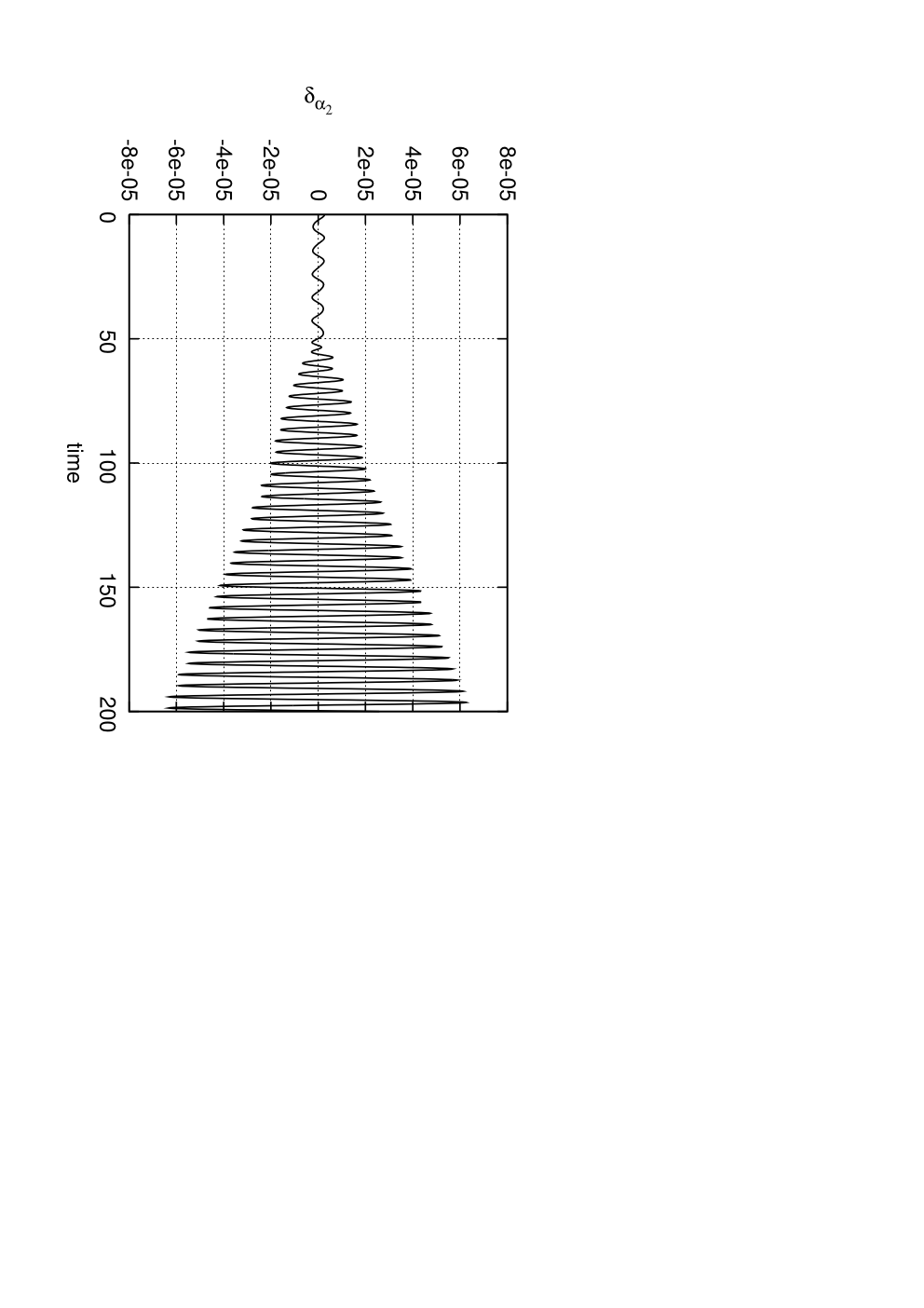
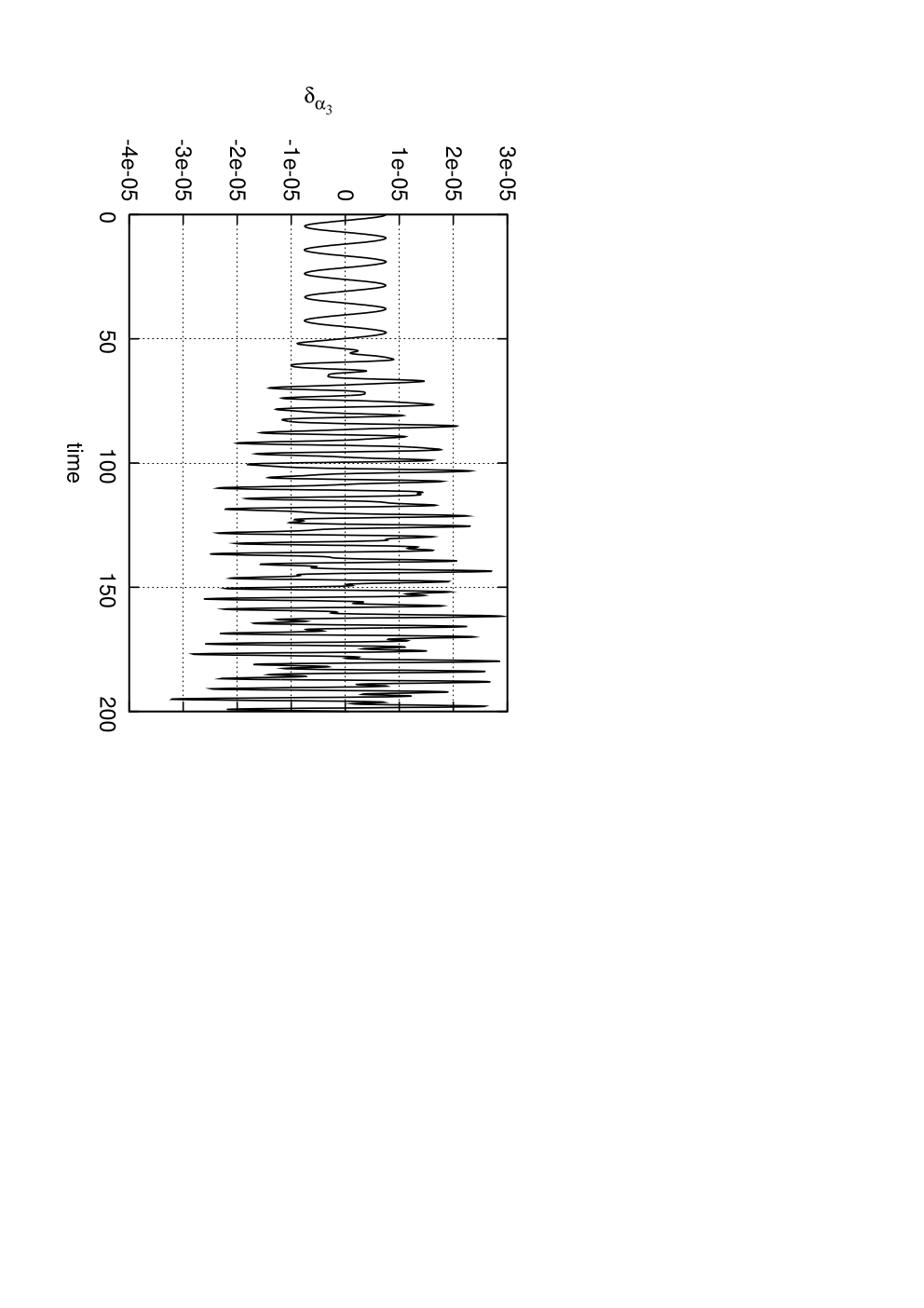
The agreement is excellent and the error of about is essentially the error in the trapeze method . If only the first three modes are used in the amplitude equations, the error is still very small. In many other cases, we compared the solution of the full problem (10) with the one given by the amplitude equations (49) and always found errors of about . This shows that these simple amplitude equations are a precise way to describe the complex system film/cavity.
After this validation, we examine the role of the forcing frequency and show that we can transfer energy from one cavity mode to another by acting on the film via the forcing and damping (52). The value of the forcing frequency is essential as shown in the following pictures. First we chose so that we are forcing the system to resonate in the second normal mode. The energy transfer is then efficient and after a short time of forcing we find the system in the normal mode 2 with very little left of the normal mode 1. This is shown in Fig. 9 where we plot the initial mode in dashed line and the newly generated mode in continuous line. This notation will be used throughout this section.

We now change the forcing frequency to and retain otherwise the same protocol. In this case we do not have a resonance of the system and it responds by generating components on the neighboring normal modes. When forcing the system on the sine Fourier mode for which no energy is fed into this mode as expected from the amplitude equations (49). The system responds on the 1st, 2nd and 4th normal modes.

We have forced the system at frequency and obtained conversion from mode 1 to mode 6. This is shown in Fig. 10. If we choose closer to the transfer is even better so that the amplitude of the mode 6 is larger. Note that it is also possible to obtain down conversion of modes. For example starting with mode 6 and forcing at a frequency we obtain the mode 1 and a little of mode 2. This is shown in Fig. 11.

The value of determines the efficiency of conversion to or from the mode . For example with a cavity of length and a film placed at , we find and . We can then state that in general, conversion from modes close to to normal modes far from is more efficient than the converse. This is because in the amplitude equations (49) the damping of is proportional to while the amplification term is proportional to . So a mode close to resonance with a large is damped more than another normal mode with a smaller . This is shown in Fig. 10 and 11.
To summarize we have shown that this linear system can convert energy from one normal mode to another. This was thought impossible for a linear system because of the orthogonality of the normal modes. Here because we act on the sub-system we are able to do this transfer. Another important result is the excellent agreement between the solution of the amplitude equations and the solutions of the initial problem. This simple method could then be used in practice to solve the singular partial differential equation (10).
6.2 Nonlinear regime
Another way to convert energy from one mode to another is through nonlinearity. A well known example is the famous study of Fermi, Pasta and Ulam (see for example the entry in [27]) showing energy recurrence between Fourier modes in a chain of anharmonic oscillators. Now we consider the film to follow a law with a cubic nonlinearity and take out the driving and damping terms.
The film equation now incorporates a cubic nonlinearity so that the composite cavity/film is described by the system (8). The cubic term can be treated as in the previous section and incorporated into the term of equation (42). The scalar product is
| (53) |
Then the amplitude equations are
| (54) | |||||
| (55) | |||||
If there is in addition forcing and damping on the system, one needs to add to the right hand side of (54) the terms on the right hand side of (49).
As the amplitude of the film polarization increases, one expects that higher and lower frequency normal modes will be excited. This coupling to the other modes is clear from the right hand side of the amplitude equations (54). Of course one should not increase too much the amplitude of the forcing because then the wave length of the cavity modes would reduce and become comparable with the film thickness. Then approximating the film by a Dirac distribution would not make sense.
We start the system in the first normal mode with zero amplitude and a positive velocity and let it evolve from 0. This procedure is chosen so as not to create a shock in the system with the nonlinearity. For small velocities, there is little transfer from the first to the second and third modes. Again the sine Fourier modes do not play any role because for them . Increasing the initial velocity increases the transfer of energy to the higher modes. For an velocity of 0.5, Fig. 12 shows the evolution of as a function of time for both the full system () and the amplitude equations (54).

As expected the nonlinearity generates higher frequencies. Notice the excellent agreement between the solution of the partial differential equation system and the amplitude equations. This holds even for such large velocities as 2.
We conclude this section with an observation of recurrence similar to what happens for the Fermi-Pasta-Ulam system. Fig. 13 presents a short time evolution of the first 6 modes for an initial velocity of 0.5, starting from the first mode. In the plots of Fig. 13 are superposed 4 other time evolutions taken at times where and is an integer.


This recurrence could indicate that our system is close to being integrable.
7 Conclusion
We considered the interaction between an electromagnetic field in a cavity and a thin polarized dielectric film. The model is the Maxwell-Lorenz system where the medium is described by an oscillator and the coupling to the wave equation is through a Dirac delta function. We introduced normal modes which are adapted to the system film/cavity. These are well adapted to describe the time evolution of the system, unlike the standard sine Fourier modes or other Sturm Liouville modes. The normal modes composed of the field and the displacement are orthogonal with respect to a special scalar product which we introduce. The amplitude equations derived from the normal modes give an excellent description of the dynamics and could even be used as a numerical tool instead of solving the full partial differential equation system using the fairly involved finite volume method.
Assuming a linear oscillator for the film, we show conversion from one normal mode to another by forcing the film at specific frequencies. This is new for linear systems and could be used for many applications in optics or microwaves.
If the film is described by an anharmonic oscillator, the evolution generates other modes. Again the amplitude equations provide excellent agreement with the solution of the full problem. Finally we observed recurrence for certain initial velocities of the film. This phenomenon is known to exist for systems close to integrability. The fact that we observe it here may indicate that our system is in some ways close to integrability.
Acknowledgments
The authors thank André Draux and Yuri Gaididei for very useful discussions. Elena Kazantseva thanks the Region Haute-Normandie for a Post-doctoral grant. Andrei Maimistov is grateful to the Laboratoire de Mathématiques, INSA de Rouen for hospitality and support. The authors thank the Centre de Ressources Informatiques de Haute-Normandie for access to computing ressources.
References
- [1] A. C. Newell and J. V. Moloney, ”Nonlinear optics”, Addison Wesley, (1992).
- [2] H.Walther, B.T.H. Varcoe, B.-G. Englert and Th. Becker, Rep. Prog. Phys. 69 1325-1382 (2006)
- [3] B. Vasilic, E. Ott, T. Antonen, P. Barbara and C. J. Lobb Phys. Rev. B 68, 024251, (2003).
- [4] , J. G. Caputo and L. Loukitch, in ”Nonlinear waves in complex systems: energy flow and geometry”, J. G. Caputo and M. P. Soerensen Eds., Collection ”Special Topics” of European J. Phys. 147, (1), (2007).
- [5] P. Horak, G. Hechenblaikner, K. M. Gheri, H. Stecher and H. Ritsch, Phys.Rev. Lett. 79, 4974, (1997).
- [6] J.T. Shen and S. Fan, Phys. Rev. Lett. 95, 213001, (2005).
- [7] V. I. Rupasov and V. I. Yudson, Sov. J. Quantum Electronics, 12, 415, (1982).
- [8] V. I. Rupasov and V. I. Yudson, Sov. Phys. J.E.T.P. 66, 282, (1987)
- [9] Y. Ben-Aryeh, C. M. Bowden, and J. C. Phys.Rev. A34, 3917 - 3926 (1986)
- [10] , M. G. Benedict, A. I. Zaitsev, V. A. Malyshev, and E.D. Trifonov, Opt. Spectrosk. 66, 726-728 (1989)
- [11] M. G. Benedict, V. A. Malyshev, E.D. Trifonov and A. I. Zaitsev, Phys. Rev A 43, 3845, (1991).
- [12] S.O. Elyutin, A. I. Maimistov, Opt. Spectrosk. 90, 849-857 (2001)
- [13] A. M. Basharov, A. I. Maimistov, S.O. Elyutin, Zh.Eksp.Teor.Fiz. 115, 30-42 (1999)
- [14] S.O.Elyutin, A.I. Maimistov, J.Mod.Opt. 46, 1801-1816 (1999)
- [15] S.O. Elyutin, Phys.Rev. A75, 023412 (8 pages) (2007)
- [16] S.O. Elyutin, J. Phys. B: At. Mol. Opt. Phys. 40, 2533-2550 (2007)
- [17] V.A. Malyshev, I.V. Ryzhov, E.D. Trifonov, A.I. Zaitsev, Opt.Commun. 180, 59-68 (2000)
- [18] M.G.Benedict, E.D.Trifonov, Phys.Rev. A38, 2854-2862(1988).
- [19] A.M.Samson,Yu.A.Logvin, S.I.Turovets Opt.Commun 78, 208-212 (1990)
- [20] J.-G. Caputo, E. V. Kazantseva, A.I. Maimistov, Phys. Rev. B 75, 14113 (2007)
- [21] A.I. Maimistov, I.R. Gabitov, Eur. Phys. J. Special Topics 147, 265-286 (2007) in ”Nonlinear aves in complex systems: energy flow and geometry” (Springer, 2007)
- [22] R. Hildebrand, ”Advanced Calculus for applications”, Prentice Hall, (1976).
- [23] R. Courant and D. Hilbert, Methods of mathematical physics, Wiley, (1959).
- [24] H.Dong, Z.R. Gong, H. Ian, Lan Zhou, C.P. Sun, Intrinsic Cavity QED and Emergent Quasi-Normal Modes for Single Photon, arXiv:0805.3085v2 [quant-ph]
- [25] P. Bocchieri, A. Crotti and A. Loinger, A classical solvable model of a radiant cavity, Lettere al nuovo cimento, vol. 4, 741-744, (1972).
- [26] H. S. Carslaw, An introduction to the theory of Fourier’s series and integrals, Dover, (1950).
- [27] Encyclopedia of nonlinear science, A. C. Scott Editor, Taylor and Francis, (2005).
- [28] E. Hairer, S. P. Norsett and G. Wanner. Solving ordinary differential equations I, Springer-Verlag, (1987).
7.1 Appendix A: Inconsistent projection using standard eigenmodes
Using standard Sturm-Liouville eigenmodes and the usual scalar product leads to inconsistent results. To show this let us assume no forcing for simplicity. We consider the usual eigenmodes associated with the Sturm Liouville problem
| (56) |
Call these modes associated to the eigenfrequency .
One then expands the field as
Plugging this expansion into the system of equations (10) and projecting onto the using the standard scalar product, one gets the evolution of the ’s
| (57) | |||
| (58) | |||
| (59) |
Let us examine the jump condition on from the partial differential equation (10). We have
| (60) |
From the expansion (7.1), we obtain
We get the jumps of the from the eigenvalue relation
and obtain that
which is clearly inconsistent with the result obtained from the original system (60). Therefore one needs to use the normal modes associated with the full system and the special scalar product (37) to get a consistent reduced description of the system.
7.2 Appendix B: Numerical method for solving (10)
The evolution equation (10) involves a partial differential equation with a Dirac distribution coupled to an ordinary differential equation. We solve this coupled system using the method of lines where the time operator is kept as such and the space operator is discretized, naturally leading to a system of coupled ordinary differential equations. The spatial operator is a distribution so the natural way to give it meaning is to integrate it over small reference intervals (finite volume approximation). The value of the function is assumed to be constant in each volume. This method of lines allows to increase the precision of the approximation in time and space independantly.
We tranform (10) into a system of first order partial differential equations
| (61) | |||
| (62) | |||
| (63) | |||
| (64) |
We then define our volume elements making sure that is the center of one element. We then integrate the operator on each volume where is the space step. For , we recover the standard finite difference expression for the Laplacian
and get the discrete wave equation
| (65) | |||
| (66) |
For , we get
| (67) | |||
| (68) | |||
| (69) | |||
| (70) |
The coupled system (65,67) is then integrated using an ordinary differential equation solver. In practice we use the variable step Runge-Kutta 4-5 Dopri5 developped by Hairer and Norsett at the University of Geneva [28].