Funnel landscape and mutational robustness as a result of evolution under thermal noise

Under fixed conditions, biological systems evolve to increase their fitness, determined by a biological state -phenotype- that is shaped by a dynamical process. This dynamics is generally stochastic as they are subject to thermal noise, and the rule for the dynamics is controlled by a gene that mutates through generations. Those genes that produce higher fitness values have a higher chance of survival. For example, the folding dynamics of a protein or t-RNA shapes a structure under thermal noise to produce a biological function, while the rule for the dynamics is coded by a sequence of DNA.

The phenotype that provides fitness is expected to be rather insensitive to the type of noise encountered during the dynamical process [1, 2, 3], to continue producing fitted phenotypes. The first issue is to determine what type of dynamics is shaped through evolution to achieve robustness to noise. To have such robustness it is preferable to utilize a dynamical process that produces and maintains target phenotypes of high fitness smoothly and globally from a variety of initial configurations. In fact, the existence of such a global attraction in the protein folding was proposed as a consistency principle[4] and a funnel landscape[5], while similar global attraction has been discovered in gene regulatory networks[6]. Despite the ubiquity of such funnel landscapes for phenotype dynamics, little is understood on how these structures are shaped by the evolution [7, 8, 9]. The second issue we address is the conditions under which funnel-like dynamics evolves.

Besides its robustness to noise, the phenotype is also expected to be robust against mutations in the genetic sequence encountered through evolution. Despite recent studies suggesting a relationship between robustness to thermal noise and robustness to mutation[1, 10, 11, 12, 13], a theoretical understanding of the evolution of the two is still insufficient. The question of whether robustness to thermal noise also leads to robustness to mutation constitutes the third issue discussed in this paper. All these questions concerning robustness to noise and mutation or the shaping of the funnel-like landscape can be answered by introducing an abstract statistical-mechanical model of interacting spins, whose Hamiltonian evolves over generations to achieve a higher fitness.

Let us consider a system of $N$ Ising spins interacting globally. In this model, configurations of spin variables $S_{i}$ and an interaction matrix $J_{ij}$ with $i,j=1,\cdots,N$ represent phenotype and genotype, respectively. For simplicity, $J_{ij}$ is restricted to the two values $\pm 1$ and is assumed to be symmetric: $J_{ij}=J_{ji}$. The dynamics of the phenotype denoted by $\bm{S}$ is given by a flip-flop update of each spin with an energy function, defined by the Hamiltonian $H(\bm{S}|\bm{J})=-\frac{1}{\sqrt{N}}\sum_{i<j}J_{ij}S_{i}S_{j}$, for a given set of genotypes denoted by $\bm{J}$. We adopt the Glauber dynamics as an update rule, where the $N$ spins are in contact with a heat bath of temperature $T_{S}$. After the relaxation process, this dynamics yields an equilibrium distribution for a given $\bm{J}$, $P(\bm{S}|\bm{J},T_{S})=e^{-\beta_{S}H(\bm{S}\mid\bm{J})}/\penalty Z_{S}(T_{S})$, where $\beta_{S}=1/\penalty T_{S}$ and $Z_{S}(T_{S})=\mbox{Tr}_{\bm{S}}\exp[-\beta_{S}H(\bm{S}|\bm{J})]$.

The genotype $\bm{J}$ is transmitted to the next generation with some variation, whereas genotypes that produce a phenotype with a higher level of fitness are selected. We assume that fitness is a function of the configuration of target spins $\bm{t}$, a given subset of $\bm{S}$, with size $t$. The time-scale for genotypic change is generally much larger than that for the phenotypic dynamics, so that the variables $\bm{S}$ are well equilibrated within the unit time-scale of the slower variable $\bm{J}$. Such being the case, fitness should be expressed as a function of the target spins $\bm{S}$ averaged with respect to the distribution. Considering the gauge transformation [15], we define fitness as

without losing generality, where $\langle\cdots\rangle$ denotes the expectation value with respect to the equilibrium probability distribution. In other words, the expected fitness is given by the probability of the “target configuration” in which all target spins are aligned parallel under equilibrium conditions. Note that in our model, only the target spins contribute to the fitness, and as a result, the spin configuration for a given fitness value has redundancy.

The genotype $\bm{J}$ evolves as a result of mutations, random flip-flop of the matrix element, and the process of selection according to the fitness function. We again adopt Glauber dynamics by using fitness instead of the Hamiltonian in the phenotype dynamics, where $\bm{J}$ is in contact with a heat bath whose temperature $T_{J}$ is different from $T_{S}$. In particular, the dynamics is given by a stochastic Markov process with the stationary distribution $P(\bm{J},T_{S},T_{J})=e^{\beta_{J}\Psi(\bm{J},T_{S})}/\penalty Z_{J}(T_{S},T_{J})$, where $\beta_{J}=1/T_{J}$ and $Z_{J}(T_{S},T_{J})=\mbox{Tr}_{\bm{J}}\exp[\beta_{J}\Psi(\bm{J},T_{S})]$. According to the dynamics, genotypes are selected somewhat uniformly at high temperatures $T_{J}$, whereas at low $T_{J}$, genotypes with higher fitness values are preferred. The temperature $T_{J}$ represents selection pressure.

Next, we study the dependence of the fitness and energy on $T_{S}$ and $T_{J}$, given by $\Psi(T_{S},T_{J})=\langle\Psi(\bm{J}|T_{S})\rangle_{J}$ and $E(T_{S},T_{J})=\langle\langle H(\bm{S}|\bm{J})\rangle\rangle_{J}$, respectively, where $\langle\cdots\rangle_{J}$ denotes the average with respect to the equilibrium probability distribution, $P(\bm{J},T_{S},T_{J})$. For the spin dynamics (unless otherwise mentioned), the exchange Monte Carlo (EMC) simulation [14] is used to accelerate the relaxation to equilibrium. Indeed, we have confirmed the equilibrium distribution for the simulations below. Two processes are carried out alternately: the equilibration of $\bm{S}$ with the EMC and the stochastic selection of $\bm{J}$ according to the fitness value estimated through the first process.

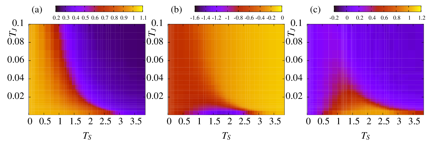
Fig. 1 (a) and (b) show dependence of the fitness and energy on $T_{S}$ and $T_{J}$, respectively, for $N=15$ and $t=3$. For any $T_{S}$, the fitness value decreases monotonically with $T_{J}$. However, $T_{S}$ influences the slope of the decrease significantly. The fitness for sufficiently low $T_{S}$ remains at a high level and decreases only slightly with an increase in $T_{J}$, while for a medium value of $T_{S}$, the fitness gradually falls to a lower level as a function of $T_{J}$ and eventually, for a sufficiently high value of $T_{S}$, it never attains a high level. This implies that the structure of the fitness landscape depends on $T_{S}$, at which the system has evolved. The energy function, on the other hand, shows a significant dependence on $T_{S}$. Although the energy increases monotonically with $T_{S}$ for high $T_{J}$, it exhibits non-monotonic behavior at a low $T_{J}$ and takes a minimum at an intermediate $T_{S}$. The $\bm{J}$ configurations giving rise to the highest fitness value generally have a large redundancy. At around $T_{S}\simeq 2.0$, using a fluctuation induced by $T_{S}$, a specific subset of adapted $\bm{J}$’s giving rise to lower energy is selected from the redundant configurations with higher fitness.

In the medium-temperature range, such $\bm{J}$s that yield both lower energy and higher fitness are evolved. Now we study the characteristics of such $\bm{J}$s. According to statistical physics of spin systems, triplets of interactions that satisfy $J_{ij}J_{jk}J_{ki}<0$ are known to yield frustration, which is an obstacle to attaining the unique global energy minimum [15]. In our model, however, the target spins play a distinct role. Hence, it becomes necessary to quantify the frustration by distinguishing target and non-target spins. In accordance with the “ferromagnetic” fitness condition for target spins, we define $\Phi_{1}$ as the frequency of positive coupling among target spins, $\Phi_{1}(T_{S},T_{J})=\frac{2}{t(t-1)}\Big\langle\sum_{i<j\in\bm{t}}J_{ij}\Big\rangle_{J}$. Under ferromagnetic coupling, the target configurations are energetically favored, i.e., $\Phi_{1}=1$, for which no frustration exists among the target spins. Next, for a measure of the degrees of frustration between target and non-target spins, and among non-target spins themselves, we define $\Phi_{2}$ and $\Phi_{3}$ as

and

where $C^{N-t}_{2}$ is the total number of possible pairs among the non-target spins. Here, $\Phi_{2}$ is the fraction of the interaction pairs between target and non-target spins that satisfy $J_{ik}J_{kj}=1\ (i,j\in\bm{t},\ k\in\hskip-8.99994pt/\ \bm{t})$. If $\Phi_{2}=1$, no frustration is introduced by the interaction between target and non-target spins, so that the energy minimum of the target configuration is conserved by such interaction. If $\Phi_{3}=1$, the target configurations do not introduce frustration in $J_{kl}$s $(k,l\in\hskip-8.99994pt/\ \bm{t})$. If $\Phi_{1}=\Phi_{2}=\Phi_{3}=1$, there is no frustration at all over the interactions, as suggested by the Mattis model [17], which can be transformed into ferromagnetic interactions by gauge transformation [15].

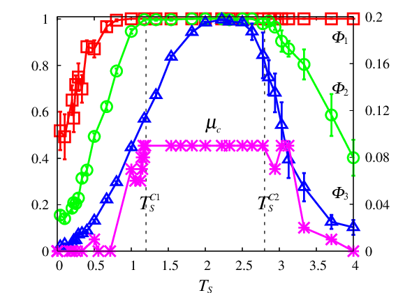
For $\bm{J}$ that is evolved under given $T_{S}$ and $T_{J}$, we have computed $\Phi_{1},\Phi_{2}$ and $\Phi_{3}$. Fig. 2 shows the dependence of $\Phi_{1},\Phi_{2}$ and $\Phi_{3}$ on $T_{S}$ at a fixed $T_{J}=0.5\times 10^{-3}$. For $T_{S}\geq T_{S}^{c1}$, $\Phi_{1}$ takes the value $\sim 1$ [16], so that a target configuration is embedded as an energetically favorable state, while no specific patterns, apart from the target, are embedded in the spin configuration.

For $T_{S}^{c1}\leq T_{S}\leq T_{S}^{c2}$, $\Phi_{2}$ also takes the value around 1, implying that frustration is not introduced by means of interactions with a non-target spin. In this temperature range, $\Phi_{3}$ is not equal to 1, except for $T_{S}\sim 2.0$ where the Mattis state is shaped. When $\Phi_{2}\sim 1$ and $\Phi_{3}\neq 1$, frustration is not completely eliminated from the non-target spin interactions, in contrast to the Mattis state. Here, such a $\bm{J}$ configuration without frustration around the target spins (but with frustration between non-target spins) is referred to as “local Mattis state” (LMS), as characterized by $\Phi_{1}=\Phi_{2}\sim 1$ and $\Phi_{3}\neq 1$. The interactions $\bm{J}$ that form such LMSs arise as a result of the evolution at $T_{S}^{c1}\leq T_{S}\leq T_{S}^{c2}$, where both a fitted target configuration and a lower energy level are achieved. As shown in Fig. 1(c), the $T_{S}$ range in which LMS is shaped becomes narrower with an increase in $T_{J}$[18]. For sufficient low $T_{J}$, there are three phases: $T_{S}<T_{S}^{c1}(T_{J})$, the phase in which frustration remains in spite of adaptation; $T_{S}^{c1}(T_{J})\leq T_{S}\leq T_{S}^{c2}(T_{J})$, the phase giving LMSs; $T_{S}>T_{S}^{c2}(T_{J})$, the phase in which no adaptation and frustration is seen.

Let us consider the relaxation dynamics of spins for each $\bm{J}$ adapted through evolution under a given $T_{S}$ and $T_{J}$, denoted as $\bm{J}^{adp}_{T_{S}}$, where $T_{J}$ is fixed at $0.5\times 10^{-3}$. To understand how the relaxation dynamics depends on $\bm{J}^{adp}_{T_{S}}$, instead of using EMC, we adopt standard MC by with the temperature $T_{S}^{\prime}$, fixed at $10^{-5}$, independently of $T_{S}$ used in obtaining $\bm{J}^{adp}_{T_{S}}$. We compute the temporal change of the target magnetization $m_{t}=|\sum_{i\in\bm{t}}S_{i}|$. Relaxation dynamics of $\langle m_{t}\rangle_{0}$ for $\bm{J}^{adp}_{T_{S}}$, $T_{S}=10^{-3}(\leq T_{S}^{c1})$, and $T_{S}=2.0(T_{S}^{c1}\leq T_{S}\leq T_{S}^{c2})$ are plotted in Fig. 3, where $\langle\cdots\rangle_{0}$ denotes the average over the randomly chosen initial conditions. As shown in Fig. 3, the relaxation process for $\bm{J}^{adp}_{T_{S}}$ evolved at low temperatures is much slower. Furthermore, $\langle m_{t}\rangle_{0}$ converges to a value $m_{t}^{\ast}$ lower than 1 and remains at that value for a long time. Depending on the initial condition, the spins are often trapped at a local minimum, so that the target configuration is not realized over a long time span.

Such dependence on initial conditions is not observed for $\bm{J}^{adp}_{T_{S}}$ for $T_{S}>T_{S}^{c1}$, where $\langle m_{t}\rangle_{0}$ approaches 1 somewhat quickly. From an estimate of the convergent value of the target magnetization $m_{t}^{\ast}$ within the above MC time scale, we obtain the relaxation time $\tau$ by fitting to the function $\langle m_{t}\rangle_{0}(s)=m_{t}^{\ast}+c\exp(-s/\penalty\tau)$, where $s$ is the MC step of the spin dynamics. The parameters $m_{t}^{\ast}$ and $\tau$ are plotted against $T_{S}$ in the inset of Fig. 3, which shows the increase of $\tau$ and the decrease of $m_{t}^{\ast}$ from 1 with the decrease of $T_{S}$ below $T_{S}^{c1}$. These results imply that the energy landscape for the interaction $\bm{J}^{adp}_{T_{S}}$ is rugged for $T_{S}\leq T_{S}^{c1}$, as in a spin-glass phase, whereas it is smooth around the target for $T_{S}^{c1}\leq T_{S}\leq T_{S}^{c2}$. Thus, this landscape is interpreted as a typical funnel landscape. It demonstrates a transition from the spin-glass phase to the funnel at $T_{S}^{c1}$ (see also [7]).

Now, in the evolved genotypes, let us examine the robustness that represents the stability of $\bm{J}$’s fitness with respect to changes in the $\bm{J}$ configuration. From the adopted genotype $\bm{J}^{adp}_{T_{S}}$, mutations are imposed by flip-flopping the sign of a certain fraction of randomly chosen matrix elements in $\bm{J}^{adp}_{T_{S}}$. The value of the fraction represents the mutation rate $\mu$. We evaluate the fitness of the mutated $\bm{J}^{adp}_{T_{S}}(\mu)$ at $T_{S}^{\prime}=10^{-5}(\neq T_{S})$, i.e., $\Psi(\bm{J}^{adp}_{T_{S}}(\mu)|T_{S}^{\prime}=10^{-5})$, by taking an average over 150 samples of mutated $\bm{J}^{adp}_{T_{S}}(\mu)$. Fig. 4 shows $\mu$ dependence of the fitness for $T_{S}=10^{-4}$ and $T_{S}=2.0$. For low values of $T_{S}$, the fitness of mutated $\bm{J}^{adp}_{T_{S}}(\mu)$ exhibits a rapid decrease with respect to the mutation rate, but for $T_{S}$ between $T_{S}^{c1}$ and $T_{S}^{c2}$, it does not decrease until the mutation rate reaches a specific value. We define $\mu_{c}(T_{S})$ as the threshold point in the mutation rate beyond which the fitness $\Psi(\bm{J}^{adp}_{T_{S}}(\mu)|T_{S}^{\prime})$ begins to decrease from unity. Fig. 2 shows the dependence of $\mu_{c}$ on $T_{S}$, which has a plateau at $T_{S}^{c1}\leq T_{S}\leq T_{S}^{c2}$ where $\Phi_{2}$ is unity. This range of temperatures that exhibits mutational robustness agrees with the range that gives rise to the LMS. In other words, mutational robustness is realized for a genotype with no frustration around the target spins. Evolution in a mutationally robust genotype $\bm{J}$ is possible only when the phenotype dynamics is subjected to noise within the range $T_{S}^{c1}\leq T_{S}\leq T_{S}^{c2}$. This mutational robustness is interpreted as a consequence that the fitness landscape becomes non-neutral for $T_{S}\geq T_{S}^{c1}$ [18].

To check the generality of the transition to the LMS as well as the mutational robustness, we have examined the model by increasing the number of target spins $t$, and confirmed that the LMSs evolve at an intermediate range of $T_{S}$ (that depends on $t$), where both lower energy and higher fitness are realized together with mutational robustness, while the actual fitness value therein decreases with an increase in $t$. Simulations with larger $N$ (up to 30) have also confirmed the evolution of the LMSs at an intermediate range of $T_{S}$ [18].

In this study, in order to elucidate the evolutionary origin of robustness and funnel landscape, we have considered the evolution of a Hamiltonian system to generate a specific configuration for target spins. The findings can be summarized as follows. First, as a result of the formation of a funnel landscape through the evolution of the Hamiltonian, robustness to guard against noise is achieved in the dynamic process. Such shaping of dynamics is possible only under a certain level of thermal noise, given by temperatures $T_{S}^{c1}\leq T_{S}\leq T_{S}^{c2}$. Second, under such a temperature range in the process, a funnel-like landscape that gives rise to a smooth relaxation dynamics toward the target phenotype is evolved to avoid the spin-glass phase. This may explain the ubiquity of such funnel-type dynamics observed in evolved biological systems such as protein folding and gene expression [12, 6]. Third, this robustness to thermal noise induces robustness to mutation; this observation has also been discussed for gene transcription network models [12]. Relevance of thermal noise to robust evolutions is thus demonstrated.

The funnel-like landscape evolved at $T_{S}^{c1}\leq T_{S}\leq T_{S}^{c2}$ is characterized by the local Mattis state without frustration around the target spins. This allows for a smooth and quick relaxation to the target configuration, which is in contrast with the relaxation on a rugged landscape in spin-glass evolved at $T_{S}<T_{S}^{c1}$, where relaxation is often trapped into metastable states. Theoretical analysis of random spin systems such as replica symmetry breaking will be relevant to the local Mattis state and mutational robustness [18], as the model discussed in this letter is a variant of spin systems with two temperatures [19].