737 \Yearpublication2008\Yearsubmission2008\Month6\Volume329\Issue7\DOI10.1002/asna.200811018
2008 Aug 30
Numerical experiments on dynamo action in sheared and rotating
turbulence
Abstract
Numerical simulations of forced turbulence in elongated shearing boxes are carried out to demonstrate that a nonhelical turbulence in conjunction with a linear shear can give rise to a mean-field dynamo. Exponential growth of magnetic field at scales larger than the outer (forcing) scale of the turbulence is found. Over a range of values of the shearing rate spanning approximately two orders of magnitude, the growth rate of the magnetic field is proportional to the imposed shear, , while the characteristic spatial scale of the field is . The effect is quite general: earlier results for the nonrotating case by ( ) Yousef et al. (2008) are extended to shearing boxes with Keplerian rotation; it is also shown that the shear dynamo mechanism operates both below and above the threshold for the fluctuation dynamo. The apparently generic nature of the shear dynamo effect makes it an attractive object of study for the purpose of understanding the generation of magnetic fields in astrophysical systems.
keywords
magnetic fields – magnetohydrodynamics (MHD) – turbulence1 Introduction
Turbulence is generally considered to play a fundamental role in the generation and maintenance of magnetic fields found in a wide range of astrophysical systems. It is a numerically well established property of turbulence to amplify magnetic fluctuations at the same or smaller scales than the scales of the turbulent motions (Meneguzzi, Frisch & Pouquet 1981; Schekochihin et al. 2004; Haugen, Brandenburg & Dobler 2004; Iskakov et al. 2007; Schekochihin et al. 2007). This type of dynamo is known as small-scale, or fluctuation, dynamo. It is believed to be a universal property of turbulent systems and, at least in the case of large magnetic Prandtl numbers, a simple theoretical picture exists of the field amplification via random stretching by turbulent motions (Moffatt & Saffman 1964; Zel’dovich et al. 1984; see also Schekochihin et al. 2004; Schekochihin & Cowley 2007). It often turns out to be more difficult to either establish or explain the generation of magnetic fields at much larger scales than the turbulence scale. Such fields are observed or believed to exist in many astrophysical bodies (stars, galaxies, disks), so the question of their origin is an important theoretical challenge.
Mechanisms for the generation of such large-scale fields are known as large-scale, or mean-field, dynamos. A motley of such mean-field dynamos has been studied in the literature (Moffatt 1978; Krause & Rädler 1980; Brandenburg & Subramanian 2005; Rädler & Rheinhardt 2007, e.g.,). The precise way in which they operate often seems to be system dependent and introducing ever more realistic features into one’s theoretical model produces ever more complicated behaviour. While such modelling is necessary for quantitative understanding, it is quite interesting to ask what are the generic ingredients required to produce large-scale fields. One such ingredient appears to be the presence of net kinetic helicity in the system: in many mean-field dynamos, the key generation mechanism is the so-called effect (Steenbeck, Krause & Rädler 1966), whereby an assembly of non-mirror-symmetric velocity fluctuations having a nonzero net helicity are responsible for magnetic-field generation. The existence of a mean-field dynamo in helically forced turbulence is well established numerically (Brandenburg 2001; Maron & Blackman 2002; Brandenburg et al. 2008b). However, the requirement of net helicity may somewhat limit the applicability of the effect. It is also far from certain that the direct link between kinetic helicity and mean-field generation via the effect found in the model case where the helicity is injected by the random forcing, carries over to the cases where the helicity arises naturally (e.g., in a rotating convective layer; see Cattaneo & Hughes 2006). Therefore, there is a strong motivation for seeking alternative mean-field dynamo processes driven by nonhelical turbulence.
It is clear that a nonhelical turbulence by itself cannot make large-scale fields. In recent years, many authors have argued that large-scale magnetic fields can be generated by nonhelical velocity fluctuations when acted upon by a large-scale shear: theoretical paradigms put forward to support such a dynamo, which we refer to as the shear dynamo, have included the shear-current effect (Rogachevskii & Kleeorin 2003; Rogachevskii & Kleeorin 2004), the stochastic effect (Vishniac & Brandenburg 1997; Silant’ev 2000; Fedotov 2003; Fedotov, Bashkirtseva & Ryashko 2006; Proctor 2007; Brandenburg et al. 2008a; see, however, Kleeorin & Rogachevskii 2008), negative-diffusivity type theories (Urpin 1999a; Urpin 1999b; Rüdiger & Urpin 2001; Urpin 2002; Urpin 2006), shear amplification of the fluctuation-dynamo-generated small-scale fields (Blackman 1998). While there is not yet agreement between theoreticians about the validity or areas of practical applicability of these models, it is clear that they are addressing a fundamental issue. Indeed, shear is an extremely generic property of astrophysical systems, so the idea of a shear dynamo gives us a particularly attractive scenario for ubiquitous generation of large-scale magnetic fields.
Until recently, a numerical demonstration of this type of dynamo remained elusive. Originally motivated by the predictions of Rogachevskii & Kleeorin (2003); Rogachevskii & Kleeorin (2004), we have previously performed numerical simulations of nonhelical turbulence with a superimposed linear shear and demonstrated the existence of the shear dynamo (Yousef et al. 2008). Theoretical understanding of these numerical results is still poor. More work and, we believe, more information gathered from numerical experiments are needed in order to make progress towards understanding the properties of this dynamo and the underlying physical processes that produce it. This paper, which is an extension of the work by Yousef et al. (2008), aims at presenting a collection of new numerical results regarding the existence and behaviour of the shear dynamo in various regimes. We focus on three different cases of astrophysical interest, namely shear dynamo in the presence of forced nonhelical turbulence and a linear velocity shear, shear dynamo in the presence of forced nonhelical turbulence and Keplerian differential rotation, and finally shear dynamo in the presence of forced nonhelical turbulence, Keplerian differential rotation and a small-scale fluctuation dynamo. In order to study the effects of shear and rotation, we adopt a local rotating shearing sheet model. This model and the corresponding numerical set-up are presented in Sect. 2. In Sect. 3, we consider the case of linear shear without rotation. Results for the Keplerian regime are presented in Sect. 4. Section 5 describes some preliminary results on the shear dynamo in the presence of small scale magnetic fluctuations generated by the fluctuation dynamo. A short discussion concludes the paper (Sect. 6).
2 Model and numerical set up
We consider differentially rotating flows that can locally be described in terms of a background shear flow rotating uniformly with a rotation rate . In the framework of incompressible magnetohydrodynamics (MHD), solenoidal velocity and magnetic field perturbations to this flow evolve according to the following equations written in the rotating frame:
| (1) | |||||
| (2) | |||||
where , is the velocity deviation from the background flow , is the magnetic field normalised by , is the density, is the pressure determined by requiring , and and are the kinematic viscosity and magnetic diffusivity coefficients, respectively.
Using this local formulation allows us to study different instances of differentially rotating background flows by changing the values of the shearing and rotation rates and . In this paper, we consider two important cases: (a) shear with no rotation, , (see Sect. 3) and (b) Keplerian rotation, (see Sect. 4). The nonrotating case has been discussed by us previously (Yousef et al. 2008) and is relevant to nonrotating systems as well as systems where one expects the shear to be stronger than the rotation (one good astrophysical example is irregular galaxies, where large-scale magnetic fields are found in the absence of strong overall rotation;11 1 We thank D. Sokoloff for pointing this out to us. see Chyży et al. 2000; Chyży et al. 2003; Gaensler et al. 2005; Kepley et al. 2007). The case of Keplerian rotation corresponds to the local shearing-sheet model of thin accretion disks, for which the angular velocity decreases radially . It is commonly used to study turbulence and transport in accretion disks, in particular the MHD turbulence driven by the magneto-rotational instability (MRI) (see, e.g., Balbus 2003; Fromang et al. 2007; Lesur & Longaretti 2007, and references therein).
| Run | Resolution | 11 1 This is actually . The reported values differ from the corresponding numbers in ( ) Yousef et al. 2008. where we computed (fields averaged over and ) instead of (as erroneously claimed there). | ||||||
|---|---|---|---|---|---|---|---|---|
| S1 | 0 | 8 | 0.0161 | 3.7 | 11.5 | |||
| S2 | 0 | 16 | 0.021 | 3.8 | 11.1 | |||
| S3 | 0 | 8 | 0.0030 | 4.6 | 10.0 | |||
| S4 | 0 | 16 | 0.0124 | 5.4 | 10.2 | |||
| S5 | 0 | 32 | 0.0092 | 5.2 | 9.9 | |||
| S6 | 0 | 64 | 0.0121 | 5.1 | 9.5 | |||
| S7 | 0 | 16 | 0.0040 | 6.8 | 9.1 | |||
| S8 | 0 | 32 | 0.0058 | 7.1 | 9.0 | |||
| S9 | 0 | 64 | 0.0055 | 7.3 | 9.0 | |||
| S10 | 0 | 64 | 0.0025 | 9.7 | 8.3 | |||
| S11 | 0 | 128 | 0.0025 | 9.9 | 8.2 | |||
| S12 | 0 | 64 | 0.00094 | 13.1 | 8.1 | |||
| S13 | 0 | 128 | 0.00092 | 13.5 | 8.1 | |||
| K1 | 32 | 0.0067 | 7.0 | 8.9 | ||||
| K2 | 16 | 0.0174 | 5.0 | 9.7 | ||||
| K3 | 8 | 0.038 | 3.5 | 10.7 | ||||
| K4 | 8 | 0.086 | 2.6 | 12.7 | ||||
| K5 | 8 | 0.118 | 2.2 | 20 | ||||
| K6 | 8 | 0.147 | 2.1 | 44 | ||||
| K7 | 8 | 0.078 | 2.3 | 137 | ||||
| K8 | 8 | 0.036 | 2.9 | 520 | ||||
| FD1 | 8 | 0.3222 2 Calculated for the kinematic regime of the fluctuation dynamo (where . Refer to Fig. 9 (left panel) for time evolution of and for runs FD1–FD2. | 5.833 3 Calculated for period after saturation of the fluctuation dynamo (). | 16.433 3 Calculated for period after saturation of the fluctuation dynamo (). | ||||
| FD2 | 0 | 8 | 0.2922 2 Calculated for the kinematic regime of the fluctuation dynamo (where . Refer to Fig. 9 (left panel) for time evolution of and for runs FD1–FD2. | – | – |
We solve Eqs. (1) and (2) in a shearing periodic computational domain by means of a Lagrangian spectral method (Ogilvie 1998; Lithwick 2007). In our model, we use a random body force that is nonhelical satisfying -correlated in time (white noise), and has a characteristic length scale . Choosing to be -correlated in time makes it possible to impose the average injected power precisely. Here and in what follows, angular brackets denote volume averaging, while overbars represent time averaging. The characteristic outer scale length of the turbulence excited by our random body force is and for a given viscosity, the corresponding outer scale velocity is then determined by ; for sufficiently small viscosities, dimensionally, we must have .
In astrophysical systems, where the source of the turbulence is often related to the large-scale shear itself, the most relevant case tends to be , where is the turnover time of the turbulent motions at the outer scale. In our model, we have control over the turbulence via the parameters of the body force described above. This allows us to consider a range of values of . Such a study is useful because is only an order-of-magnitude relation (so it is not obvious which precise value of would be the most “realistic”) and also because any analytic theory of the shear dynamo would have to predict how the effect depends on the value of (usually it is only the asymptotic case that can be treated analytically, as, e.g., in Rogachevskii & Kleeorin 2003; Rogachevskii & Kleeorin 2004).
As we shall see, a significant separation in scales between and the dimensions of the computational domain is necessary to get magnetic field growth—this is particularly true for weak shears. Also very long run times (at least hundreds and, for weak shears, thousands of turnover times) are needed to get reliable statistics. This is computationally expensive and we were only able to satisfy both requirements within available computational resources by restricting our study to computational domains elongated in the direction. Thus, in all the runs presented here, we have , the forcing scale is and is taken to be between and (depending on the value of ), so . The minimum value of needed for a given simulation to produce results independent of the box size in the direction depends on the shearing rate (this issue is discussed in Sect. 3.3). Setting together with defines the code units of length and time.
A list of all runs is given in Table 1. The S (sheared, nonrotating) and K (Keplerian) runs have . The S runs have while the K runs have (larger velocities in the former case are due to the excitation of large-scale velocity structures in the absence of rotation; see Sect. 3.4). This corresponds to Reynolds numbers and for the S and K runs, respectively. The magnetic Reynolds number for all runs, as the study of the dependence of the shear dynamo properties on the magnetic Prandtl number lies outside the scope of this paper. As the Reynolds numbers are low, only relatively low resolution is needed and we find it sufficient to have 32 collocation points per code unit of length. Strictly speaking, this is not fully developed turbulence as there is little, if any, separation between the energy-containing (outer) and viscous scales. However, this is not a serious limitation because one expects the mean field dynamo mechanism and the properties of the resulting mean field to depend only on the outer scale of the turbulence (rather than on the structure of the inertial-range) and, therefore, to become asymptotically independent of for some critical While one cannot, of course, always take this kind of intuition for granted, one expects it to work at least for a turbulence driven with fixed input power as in our simulations. It does, indeed, appear to work: by rerunning a selection of the runs with lower viscosity, we have confirmed that the results reported below are independent of .
All simulations start with a dynamically insignificant random seed magnetic field whose volume average is (and remains) zero. The initial magnetic energy is for runs S1–S13 and for runs K1–K8 and FD1–FD2. The shear dynamo mechanism generates a magnetic field with large-scale structure in the direction. The field grows exponentially until it reaches a saturated state, in which the value of becomes comparable to . In this paper, we only analyse the kinematic regime of this dynamo, in which the back reaction of the magnetic field onto the velocity field through the Lorentz force can be neglected, and so only consider data for times before reaches . All numbers reported in Table 1 are for this kinematic stage, except for the run FD1 (see Sect. 5).

Before we close this section, several important remarks are in order, concerning the physical effects that are not present in our simulations.
First, the magnetic Reynolds numbers for all runs except FD1 and FD2 are deliberately chosen to lie below the critical threshold value at which the fluctuation dynamo sets in. This ensures that the magnetic-field growth observed in the S and K runs is a result of a “pure” mean-field dynamo, unpolluted by the fluctuation dynamo and that the operation of the former is not predicated on the existence of the latter.
Second, the magnetorotational instability, MRI turbulence or MRI dynamo are not present in the Keplerian runs K and FD1. This is because the magnetic field is extremely weak (in the K runs) and the viscosity is large. In addition, we know that the MRI dynamo and turbulence have so far only been found for values of systematically larger than unity, in high-resolution simulations of Keplerian shearing boxes elongated in the direction (Fromang et al. 2007; Lesur & Ogilvie 2008).
Third, the turbulence in all our simulations is statistically nonhelical, even for the runs with rotation. The kinetic helicity has a zero time average, , and only fluctuates on the turbulent time scales (). This is a consequence of being nonhelical, , and -correlated in time. The latter guarantees that the time average of helicity production is . Figure 1 shows the time evolution of for a typical run. This excludes the possibility that effect, at least in its standard and simplest form, is present in our simulations.
3 Shear dynamo without rotation
In this section, we document the numerical results obtained for and (turbulence shear, no rotation). This regime is covered by the S runs (Table 1). In all of them, we find that magnetic field grows exponentially. Let us first describe the spatial structure of this growing field, then the dependence of its properties on the shearing rate and their convergence with respect to the vertical size of the computational box.
3.1 Structure and evolution of the growing field
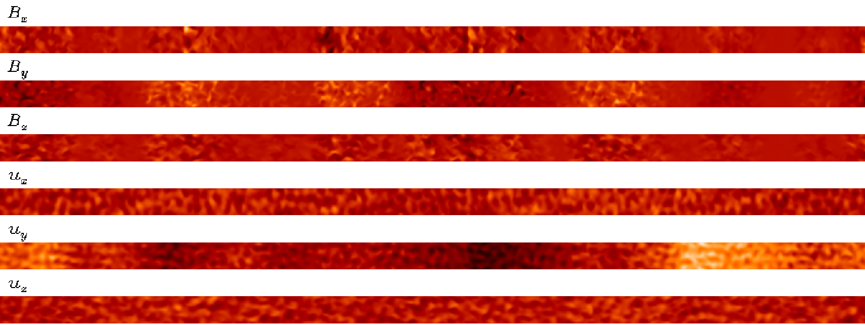

Figure 2 shows a cross section of the different components of and from a representative run with no rotation and weak shear. One can clearly distinguish between fluctuations with scales comparable to the forcing scale (which is, on the average, of the horizontal box size ) and a large-scale “mean” field. The small-scale fluctuations cannot result from the fluctuation dynamo because . Instead, they stem from the tangling of the mean field by the turbulence – the energy in these fluctuations is comparable to the energy of the mean field (for larger , this energy will be even larger; see, e.g., Schekochihin et al. 2007, and references therein).
The spatial structure of the magnetic field is illustrated by Fig. 3, which shows the time-averaged normalised spectrum of the growing field with respect to ,
| (3) |
Note that since the average forcing wave number is , where , the mean square forcing wave number associated with one spatial dimension is . The peak of the spectrum at corresponds to the mean field. The fluctuations at smaller scales are also evident, although at the low value of that we use they are not very large.

In order to systematically isolate the mean field from the small-scale fluctuations, we filter out the highest Fourier modes:
| (4) |
This is our definition of the mean field. The Fourier filtering averages out all variation in the and directions and removes the scales in the direction smaller than . Note that is strictly zero because : indeed, as the filtered field has no variation in and . Of the two nonzero components of the growing mean field, component is the larger: this can be seen in Fig. 2, where we plot the instantaneous profiles of the field components and their Fourier-filtered means. This relative predominance of is not surprising given the form of Eq. (2) where in addition to the turbulent stretching terms, there is a linear term whereby the shear systematically produces from (azimuthal field from radial field in axisymmetric systems; this is known as the -effect in dynamo theory).
As well as having a large-scale spatial coherence, the mean field is also coherent over long times. While it does not seem to be an eigenmode in the usual sense of having a shape that is exactly constant in time, the characteristic times over which it changes are much longer than both the turbulent turnover time and the shearing time . The time evolution of the mean field is illustrated by Fig. 4 (the left panels for nonrotating runs, the right panels for rotating runs; see Sect. 4). Here we plot the evolution of the profile of the component of the magnetic field averaged over and , . In all cases, we see a well-defined evolving spatial structure: patches of stronger or weaker field slowly drift along , occasionally peter out and reemerge.


3.2 Dependence on the shearing rate
Dependence of the properties of the growing field on the shearing rate is the first obvious parameter scan to carry out. It provides a quantitative test of past mean-field theories and possibly a valuable hint as to how one might construct future ones.
The dependence of the growth rate of on is plotted in the left panel of Fig. 5. The growth rates for the nonrotating runs appear to fit approximately the dependence for between and . Note, however, that the actual numerical values of are substantially smaller than (see Table 1). We do not currently know what determines the proportionality coefficient (we have checked that it is not the value of : the growth rates presented here do not change as the Reynolds number is increased).
In Table 1, we also list . Its value is approximately 10 irrespective of , although it shows a slight tendency to increase with . This is consistent with because from the component of the induction equation Eq. (2), we can estimate , so .
From Fig. 4, we already knew that the scale of the mean field decreases with shear. In order to study this dependence quantitatively, we define the characteristic length scale of the mean field as follows
| (5) |
The values of for all runs are listed in Table 1 and plotted in the right panel of Fig. 5 as a function of the shearing rate . We see that for the values of that we have studied, the characteristic length scale approximately matches the scaling . It is possible to argue (Yousef et al. 2008) that for a generic model form of mean-field equations, this scaling would indeed be consistent with the linear scaling of the growth rate, .
These scalings do not agree with the mean field theory in its current state. Namely, Rogachevskii & Kleeorin (2003), that proposed the existence of the shear dynamo using a mean-field theory with the -approximation closure to incorporate the effect of turbulence, predicted that for the fastest-growing mode and for . These scalings do not seem to match the numerical results. However, we cannot exclude the possibility that the values of considered by us are, in fact not asymptotic in the small parameter and that Rogachevskii and Kleeorin’s scalings might hold for even weaker values of shear or for numerical domains that allow more scale separation between the turbulence and the horizontal box size ( and/or ).
3.3 Independence of the computational domain size

It is important to ensure that the results reported above, particularly those of Fig. 5, are independent of the size of the computational domain. Since the growing mode has large-scale structure in the direction, we do this by performing, for each value of , a set of runs in boxes with successively larger values of until we can ascertain that the properties of the growing mode are independent of . To illustrate this procedure, the bottom panel of Fig. 6 shows the time evolution of for runs with : exponential growth with a growth rate independent of emerges as is increased. Another illustration of the convergence with respect to is Fig. 3, where normalised magnetic-energy spectra are plotted for the same runs as in Fig. 6. We see that the peak of the spectrum (corresponding to the mean field) becomes independent of at sufficiently large .
We have performed this type of study for a number of values of and in all cases confirmed convergence with respect to . This is documented in Table 1. Naturally, as the scale of the mean field decreases with increasing shearing rate (Sect. 3.2), the minimum required for convergence also decreases. Thus, we find that are sufficiently large for shearing rates and , respectively.
The convergence with respect to ensures that the properties of the mean field and their dependence on the shearing rate are physical and are not numerical artifacts related to the choice of the computational domain size in . It is also important to check whether the results depend on the dimensions of the computational domain in the and direction. Such study, which is more computationally demanding, has been left outside the scope of this paper and will be undertaken elsewhere.
3.4 Vorticity dynamo
We finally mention another noteworthy result in the nonrotating regime. We observed that the velocity field also develops energetic fluctuations with correlation times much greater than and . This property is illustrated in the top panel of Fig. 6. Since homogeneous linear shear is known to become nonlinearly unstable (see Pumir 1996, and references therein) at large enough , one might imagine that the observed velocity fluctuations result from finite-amplitude destabilisation of shear by forcing-scale motions. Indeed, for high enough values of and/or we experienced that our background shear became vigorously unstable and developed into a flow characterised by and fluctuations on all scales. However, this is not the case for any of the runs presented here. There is a key difference between these runs and the truly unstable cases. Finite-amplitude instabilities are known to feed on shear (Casciola et al. 2003) and are characterised by large correlations associated with turbulent momentum transport. This contrasts with our results: as Fig. 7 shows, there seems to be almost no correlation between the large velocity fluctuations and the mean power injected into the flow by the shear in our runs. The ratio of this shear power to the forcing power stays much smaller than unity, , implying that the velocity fluctuations feed on the forcing and not on the shear.

These observations suggest that the finite-amplitude instabilities associated with the shear are not the cause of the observed velocity fluctuations. Given the formal similarities between the induction and vorticity equations, one might argue that a “vorticity dynamo” similar to the shear dynamo is triggered (Elperin, Kleeorin & Rogachevskii 2003). This is supported by the fact that the large-scale velocity structure forms mainly in (see Fig. 2), which corresponds to the large-scale vorticity , the quantity one expects to be analogous to . The difference between the vorticity and the magnetic-field dynamos is that the “seed” field for the vorticity dynamo results from the forcing and is, therefore, never dynamically insignificant. Thus it is not possible to observe a long kinematic growth phase for this vorticity dynamo. One might conjecture that the large velocity fluctuations represent the nonlinear regime of such a dynamo. We note, however, that the status of the vorticity dynamo remains uncertain because, as seen, e.g., in Fig. 6, both the time duration of the large velocity fluctuations and their amplitude depend strongly on . Thus, unlike for the magnetic field, there is no convergence here with respect to the domain size and we must remain cautious in interpreting these results.
Finally, we observe that the emergence of the large-amplitude, long-lived, large-scale fluctuations in the velocity field does not appear to be strongly correlated with the operation of the shear dynamo: compare, e.g., the time evolution of and shown in Fig. 6. As we are about to see, the absence of these velocity fluctuations in the simulations with Keplerian rotation (see Fig. 7) does not change any of the basic properties of the shear dynamo, so we feel safe in ruling out the possibility that the large-scale velocity fluctuations are a required ingredient in the shear dynamo.
4 Shear dynamo in rotating systems
Since many astrophysical plasmas (stars, disks, galaxies) are differentially rotating, it is important to understand whether, and how, the shear dynamo is affected by imposing a uniform rotation of the system. We focus on the case of Keplerian rotation introduced in Sect. 2, because it is relevant for accretion-disk dynamos and has been extensively studied numerically in this context (e.g., Balbus 2003; Fromang et al. 2007, and references therein). This regime is thought to be nonlinearly stable from the hydrodynamic point of view (Lesur & Longaretti 2005; Ji et al. 2006; Rincon, Ogilvie & Cossu 2007), meaning that the nonlinear instabilities characteristic of nonrotating shear flows are absent. They are, indeed, absent in our simulations. Furthermore, as illustrated by Fig. 7, even the large velocity fluctuations present in the time series of for the nonrotating runs are suppressed in the case of Keplerian rotation. The suppression of these fluctuations, which were tentatively interpreted in terms of a “vorticity dynamo” in Sect. 3.4, is likely to be another consequence of the stabilising effect of Keplerian rotation on hydrodynamic motions.
As we have mentioned in Sect. 3.4, the nonlinear destabilisation of the shear for too large values of and imposed limitations on the range of values of for which shear dynamo could be studied in the nonrotating case. The absence of such destabilisation in the simulations with Keplerian rotation allows us to extend the study the shear dynamo to much higher values of than in the nonrotating case (see the K runs in Table 1).
The main conclusion of this study is that Keplerian rotation does not seem to alter the properties of the shear dynamo in any significant way. All the results concerning the growing magnetic field reported in Sect. 3, both qualitative and quantitative, continue to hold in the rotating case. The right panel of Fig. 4 shows the evolution of the large-scale field with time for three runs with rotation. It is hard to see any qualitative difference between the structure and evolution of the growing field in the rotating case and its structure in the nonrotating case shown in the left panel of the same figure. The similarity between the two cases is further demonstrated in Fig. 5, which shows that for low values of , both the growth rates and the characteristic length scales seem to follow the same scaling laws in the rotating and nonrotating cases. The numerical values of with and without rotation are quite close, although the growth rates in the presence of rotation appear to be systematically slightly higher. This small difference may result from the changes in the structure of the turbulence caused by rotation or it could be due to an additional contribution to the generation of magnetic field from other mean-field dynamo mechanisms associated with rotation: e.g., the Rädler, or , effect (Rädler 1969; Rädler, Kleeorin & Rogachevskii 2003). It is worth reemphasising in this context that the turbulent motions driven by our forcing remain nonhelical on average even in the presence of Keplerian rotation (see Fig. 1 and the discussion at end of Sect. 2), so that the rotating shear dynamo does not involve an effect in the usual sense.

Figure 5 shows that, as is increased beyond the values studied for , the scalings of the growth rate and the mean-field scale, and , continue until reaches its maximum and its minimum at . At even larger shears, the growth rate starts to decrease, as it intuitively should. Indeed, the dynamo must surely disappear in the limit of infinite shear. More precisely, in the limit when the shearing rate associated with the imposed shear is much larger than the turbulent rate of strain, , the nonlinear terms (the terms involving turbulent velocities) in the induction equation Eq. (2) become negligible—without these nonlinearities, we cannot have an exponentially growing magnetic field.
This argument suggests that the qualitative change associated with the peak of the growth rate in Fig. 5 corresponds to the transition from the weak-shear regime () to the strong-shear regime (). Quantitatively, this transition evidently occurs at . Once the imposed shear becomes stronger than the turbulent rate of strain at the forcing scale , smaller turbulent scales should come into play. In order to understand what happens when the shear is strong, one must analyse the changes that such a shear causes to the inertial-range turbulence, determine the transition scale at which the turbulent rate of strain catches up with the shear, etc. Since the numerical simulations presented here, unlike real turbulent systems, have no extended inertial range, their relevance in the strong-shear regime is questionable and we shall not discuss this regime here.
Finally, for completeness, in Fig. 8 we show the one-dimensional magnetic-energy spectra, defined by Eq. (3), for Keplerian runs with several values of shear. We see that, as is decreased, the peak of the spectrum, corresponding to the mean field, moves towards lower wave numbers (corresponding to larger scales; cf. Fig. 5). The rest of the spectrum represents magnetic fluctuations produced by the turbulent tangling of the mean field. Here, like for the nonrotating runs in Sect. 3, the tangling, or magnetic induction (see Schekochihin et al. 2007, and references therein), is the only mechanism for producing small-scale fields because is chosen below the threshold for the fluctuation dynamo.
5 Shear dynamo and fluctuation dynamo


So far, we have only discussed simulations with below the critical value for the onset of the fluctuation dynamo . This choice was made to ensure that the growth in magnetic energy is solely due to the shear dynamo, allowing us to confirm the existence of this effect, its independence of the fluctuation dynamo and to study it in a “pure” isolated form. However, astrophysical objects virtually always have large , which are expected to be far above the fluctuation dynamo threshold. Thus, any mean-field dynamo scheme aspiring to explain large-scale astrophysical fields has to work simultaneously with the fluctuation dynamo. Furthermore, the fluctuation dynamo is likely to be much faster than any mean-field dynamo because its growth rate is determined by the turbulent rate of strain associated with scales much smaller than the outer scale, so , where is the outer-scale turbulent turnover time (see discussion in Schekochihin et al. 2007, and references therein). In contrast, mean-field dynamos are typically slower than the outer-scale rate of strain, so for them, . Thus, a working mechanism for mean-field generation must operate against the background not of pure hydrodynamic turbulence but rather of magnetohydrodynamic turbulence that emerges as the saturated state of the fluctuation dynamo (Rädler, Kleeorin & Rogachevskii 2003; Rogachevskii & Kleeorin 2003; Rogachevskii & Kleeorin 2004, the approach advocated, e.g., by). It cannot be taken for granted that such a magnetohydrodynamic turbulence in conjunction with shear will still be germane to the generation of large-scale magnetic fields. It is, therefore, imperative to confirm the existence of the shear dynamo effect for in order to be able to assert its potential relevance for astrophysical situations. Here we show (as far as we know, for the first time) that a combination of linear shear and a nonhelically forced homogeneous magnetohydrodynamic turbulence (saturated state of fluctuation dynamo) can support dynamically significant large-scale magnetic fields.
For this preliminary study, we performed two runs, FD1 and FD2. For FD1, , ; for FD2, . Both runs have , and thus . This value is above the threshold for the fluctuation dynamo. In the run FD2, which is a pure homogeneous turbulence run, that is the only possible field-amplification mechanism. In contrast, run FD1 has the prerequisites for both the shear and fluctuation dynamos.
The time evolution of the magnetic field for these two runs is shown in Fig. 9. Both runs develop in a similar manner initially: the magnetic field is amplified by the fluctuation dynamo and increases by 12 orders of magnitude to a dynamically strong saturated level after a time . This growth is much faster than the growth rates associated with the shear dynamo in analogous runs without the fluctuation dynamo. The growth rate is , which is consistent with the expectation that the growth rate of the fluctuation dynamo should be comparable to the turbulent rate of strain, or stretching rate—for , this is usually the rate of strain associated with the smallest turbulence scales (see, e.g., Schekochihin et al. 2004; Schekochihin et al. 2007; Brandenburg & Subramanian 2005, and references therein), but in our case the scale separation between the outer and the viscous scale is not large, so the fluctuation-dynamo growth rate should be roughly comparable to .
As evident in Fig. 9, the two runs differ significantly after the saturation of the fluctuation dynamo. The magnetic field for the zero-shear run FD2 becomes statistically stationary and stays at small scales, while in the sheared and rotating run FD1 it develops large-scale structure. The structural difference between the runs with and without shear is displayed in the right panel of Fig. 9: whereas the zero-shear run only has small scale, short-lived turbulent fluctuations, the run with an imposed shear develops large-scale, long-lived structures, which are in many ways similar to the shear-dynamo-generated mean field in the runs without the fluctuation dynamo. The existence of large-scale structures in the case with shear can also be seen from (time-averaged normalised one-dimensional) magnetic energy spectra shown in Fig. 10. The spectrum for FD1 (,), unlike that for FD2 (), has a prominent peak at a low wave numbers corresponding to a large-scale mean field. Note that in FD1 appears to develop long-lived, large-amplitude, large-scale fluctuations that are reminiscent of those observed in for the vorticity dynamo reported in Sect. 3.4 (see the inset in the left panel of Fig. 9).
Thus, we have found that the fluctuation dynamo and the shear dynamo can coexist, giving rise both to small- and large-scale magnetic fields. It is clear that a systematic parameter study at high and is called for. It requires much larger computational resources than the relatively cheap simulations reported in this paper. Since the seed field for generating large-scale magnetic fields is now provided by the already saturated small-scale fields resulting from the fluctuation dynamo, it is never really well posed under these circumstances to consider a kinematic regime of the shear dynamo (Cattaneo & Hughes 2008, cf.). Thus, we have to confront the question of how the large-scale fields saturate and what their structure is in a fully nonlinear dynamical regime. We have left these questions outside the scope of this paper. Further investigations along these lines will be reported elsewhere.
6 Conclusion
Can nonhelical turbulence in combination with large-scale velocity shear act as a mean-field dynamo and generate magnetic fields with length scales much larger than the outer scale of the turbulence? This has been the subject of considerable recent debate (Vishniac & Brandenburg 1997; Urpin 1999a; Urpin 1999b; Silant’ev 2000; Urpin 2002; Fedotov 2003; Rogachevskii & Kleeorin 2003; Rogachevskii & Kleeorin 2004; Brandenburg 2005; Fedotov, Bashkirtseva & Ryashko 2006; Rädler & Stepanov 2006; Rüdiger & Kichatinov 2006; Rädler & Rheinhardt 2007; Proctor 2007; Brandenburg et al. 2008a; Kleeorin & Rogachevskii 2008). To our knowledge, the paper by Yousef et al. (2008) and this paper present the first set of dedicated numerical experiments that demonstrates that such a generation mechanism is feasible. However, in retrospect, one might conjecture that the shear-dynamo might have already been seen in several earlier numerical studies that combined large-scale flows, and consequently large-scale shear, with nonhelical forcing at smaller (or, in some cases, similar) scales and reported generation of magnetic fields at scales larger than the forcing scale (Brandenburg 2005; Ponty et al. 2005; Mininni et al. 2005; Shapovalov 2006).
We have carried out a suite of numerical experiments on the shear dynamo effect in vertically elongated shearing boxes and for magnetic Reynolds numbers subcritical with respect to the fluctuation dynamo. For the values of the imposed shear between and (corresponding to , where is the turnover rate of the randomly forced velocity fluctuations), we have found that the dynamo growth rate is and the characteristic length scale of the generated mean magnetic field is .
The first key result of this paper, compared with the earlier study by Yousef et al. (2008), is that the shear dynamo works both in the nonrotating case and for the case of Keplerian rotation (). There does not appear to be much difference, qualitative or quantitative, between the rotating and nonrotating cases, although perhaps it would be interesting to look at non-Keplerian cases and try to identify the role of rotation via a parameter scan in independent of the one in .
The second key result, claimed on the basis of only a preliminary study, is that the shear dynamo works both for situations that are sub- and supercritical with respect to the fluctuation (small-scale) dynamo. In the latter case, the overall magnetic energy grows very quickly due to the fluctuation dynamo effect independent of the presence of the shear. Imposing the shear on the magnetohydrodynamic turbulence resulting from the saturation of the fluctuation dynamo, leads to the emergence of magnetic fields that have spatial scales larger than the outer scale of the turbulence and that fluctuate on very long time scales compared to the turbulent turnover time.
Thus, the shear dynamo effect appears to be quite general and robust. As the combination of a shear flow and turbulence is a very common feature in astrophysical systems, the shear dynamo potentially represents a generic mechanism for making large-scale fields. While much needs to be understood about its properties before its relevance to real astrophysical systems can be more than an appealing speculation, the simplicity of the idea of the shear dynamo certainly makes it a worthwhile object of study. It is also important to determine how generic the shear dynamo is and how it combines with other large-scale features present in real astrophysical systems: various differential rotation laws, temperature and density gradients, linear instabilities, etc..
Studies in this vein are already being undertaken. For example, recent numerical experiments by Käpylä, Korpi & Brandenburg (2008) have shown that large-scale dynamo action is also possible in local simulations of magnetoconvection with imposed horizontal shear. They also report a growth rate and find large-scale dynamo action for magnetic Reynolds numbers above the critical threshold for the fluctuation dynamo. Another topical recent study is by Gressel et al. (2008), who simulated the supernova-driven galactic turbulence and found that they needed to impose a linear velocity shear to obtain the amplification of a large-scale field. These studies clearly demonstrate the key role of shear in producing a mean-field dynamo. However, in comparing their results to ours, one has to keep in mind that their simulations had rotation and vertical stratification, so the turbulence in these simulations is likely to be helical and may also host an effect.
In motivating our choice of Keplerian rotation law, we mentioned the possible relevance to accretion-disk turbulence, which is believed to be driven by the magnetorotational instability (MRI) (Balbus 2003). Given a (weak) large-scale field, the MRI will generate velocity and magnetic-field fluctuations at small scales. These fluctuations, in conjunction with Keplerian rotation and shear, must then amplify the large-scale field to close the loop. The mechanisms for such an “MRI dynamo” have been discussed and simulated for some time (Brandenburg et al. 1995; Hawley, Gammie & Balbus 1996; Fromang et al. 2007; Rincon, Ogilvie & Proctor 2007; Rincon et al. 2008; Lesur & Ogilvie 2008, e.g.,). It is tempting to observe in the context of the results reported above that a combination of small-scale turbulence (magnetohydrodynamic turbulence in the case of the MRI) and large-scale shear does indeed appear to work as a dynamo giving rise to a large-scale azimuthal magnetic field ( in the shearing sheet model). We note, however, that Lesur & Ogilvie (2008), who have analysed this process in detail, find some important differences between what happens in MRI-driven shearing sheet simulations and the forced case studied by us.
To conclude, we believe that the discovery of shear dynamo has opened a number of new and exciting avenues of research and produced some promising leads towards unravelling the ways in which cosmic magnetic fields emerge. Further investigations will help assess the range of applicability and relevance of the shear dynamo effect and the physical mechanisms that are responsible for it.
Acknowledgements.
We are grateful to E. Blackman, A. Brandenburg, L. Kitchatinov, G. Lesur, G. Ogilvie, J. Papaloizou, S. Fromang, D. Shapovalov and D. Sokoloff for important discussions. TAY, NK and IR thank Nordita for its hospitality during the Turbulence and Dynamos program and the participants of the program for discussions of the shear dynamo effect. The numerical simulations were performed on HPCF (Cambridge), DCSC (Copenhagen), NCSA (Illinois) and UKAFF. This work was supported by the UK STFC (TAY, TH and AAS) and Isaac Newton Trust (TAY and TH). We also acknowledge travel support from the Royal Society (IR), US DOE Centre for Multiscale Plasma Dynamics (TAY, TH, FR and AAS) and the Leverhulme Trust Network for Magnetized Plasma Turbulence (TH and FR).References
- Balbus (2003) Balbus, S.A.: 2003, ARA&A 41, 555
- Blackman (1998) Blackman, E.G.: 1998, ApJ 496, L17
- Brandenburg (2001) Brandenburg, A.: 2001, ApJ 550, 824
- Brandenburg (2005) Brandenburg, A.: 2005, ApJ 625, 539
- Brandenburg & Subramanian (2005) Brandenburg, A., Subramanian, K.: 2005, PhRep 417, 1
- Brandenburg et al. (1995) Brandenburg, A., Nordlund, Å., Stein, R.F., Torkelsson, U.: 1995, ApJ446, 741
- Brandenburg et al. (2008a) Brandenburg, A., Rädler, K.-H., Rheinhardt, M., Käpylä, P.J.: 2008a, ApJ 676, 740
- Brandenburg et al. (2008b) Brandenburg, A., Rädler, K.-H., Rheinhardt, M., Subramanian, K.: 2008b, ApJL, submitted, arXiv:0805.1287
- Casciola et al. (2003) Casciola, C.M., Gualtieri, P., Benzi, R., Piva, R.: 2003, JFM 476, 105
- Cattaneo & Hughes (2006) Cattaneo, F., Hughes, D.W.: 2006, JFM 553, 401
- Cattaneo & Hughes (2008) Cattaneo, F., Hughes, D.W.: 2008, MNRAS, submitted, arXiv:0805.2138
- Chyży et al. (2000) Chyży, K.T., Beck, R., Kohle, S., Klein, U., Urbanik, M.: 2000, A&A 355, 128
- Chyży et al. (2003) Chyży, K.T., Knapik, J., Bomans, D.J., Klein, U., Beck, R., Soida, M., Urbanik, M.: 2003, A&A 405, 513
- Elperin, Kleeorin & Rogachevskii (2003) Elperin, T., Kleeorin, N., Rogachevskii, I.: 2003, Phys Rev E 68, 016311
- Fedotov (2003) Fedotov, S.: 2003, Phys Rev E 68, 067301
- Fedotov, Bashkirtseva & Ryashko (2006) Fedotov, S., Bashkirtseva, I., Ryashko, L.: 2006, Phys Rev E 73, 066307
- Fromang et al. (2007) Fromang, S., Papaloizou, J., Lesur, G., Heinemann, T.: 2007, A&A 476, 1123
- Gaensler et al. (2005) Gaensler, B.M., Haverkorn, M., Staveley-Smith, L., Dickey, J.M., McClure-Griffiths, N.M., Dickel, J.R., Wolleben, M.: 2005, Sci 307, 1610
- Gressel et al. (2008) Gressel, O., Elstner, D., Ziegler, U., Rüdiger, G.: 2008, A&A 483, L35
- Haugen, Brandenburg & Dobler (2004) Haugen, N.E.L., Brandenburg, A., Dobler, W.: 2004, Phys Rev E 70, 016308
- Hawley, Gammie & Balbus (1996) Hawley, J.F., Gammie, C.F., Balbus, S.A.: 1996, ApJ 464, 690
- Iskakov et al. (2007) Iskakov, A.B., Schekochihin, A.A., Cowley, S.C., McWilliams, J.C., Proctor, M.R.E.: 2007, Phys Rev Lett 98, 208501
- Ji et al. (2006) Ji, H., Burin, M.J., Schartman, E., Goodman, J.: 2006, Nature 444, 343
- Käpylä, Korpi & Brandenburg (2008) Käpylä, P.J., Korpi, M.J., Brandenburg, A.: 2008, A&A, submitted, arXiv:0806.0375
- Kepley et al. (2007) Kepley, A.A., Mühle, S., Wilcots, E.M., Everett, J., Zweibel, E., Robishaw, T., Heiles, C.: 2007, arXiv:0708.3405
- Kleeorin & Rogachevskii (2008) Kleeorin, N., Rogachevskii, I.: 2008, Phys Rev E 77, 036307
- Krause & Rädler (1980) Krause, F., Rädler, K.-H.: 1980, Mean-Field Magnetohydrodynamics and Dynamo Theory, Pergamon Press, New York
- Lesur & Longaretti (2005) Lesur, G., Longaretti, P.-Y.: 2005, A&A 444, 25
- Lesur & Longaretti (2007) Lesur, G., Longaretti, P.-Y.: 2007, MNRAS 378, 1471
- Lesur & Ogilvie (2008) Lesur, G., Ogilvie, G.I.: 2008, A&A , accepted, arXiv:0807.1703
- Lithwick (2007) Lithwick, Y.: 2007, ApJ 670, 789
- Maron & Blackman (2002) Maron, J., Blackman, E.G.: 2002, ApJ 566, L41
- Meneguzzi, Frisch & Pouquet (1981) Meneguzzi, M., Frisch, U., Pouquet, A.: 1981, Phys Rev Lett 47, 1060
- Mininni et al. (2005) Mininni, P.D., Ponty, Y., Montgomery, D.C., Pinton, J.-F., Politano, H., Pouquet, A.: 2005, ApJ 626, 853
- Moffatt (1978) Moffatt, H.-K.: 1978, Magnetic-Field Generation in Electrically Conducting Fluids, Cambridge University Press, Cambridge
- Moffatt & Saffman (1964) Moffatt, H.K., Saffman, P.G.: 1964, PhFl 7, 155
- Ogilvie (1998) Ogilvie, G.I.: 1998, unpublished
- Ponty et al. (2005) Ponty, Y., Mininni, P.D., Mongomery, D.C., Pinton, J.-F., Politano, H., Pouquet, A.: 2005, Phys Rev Lett 94, 164502
- Proctor (2007) Proctor, M.R.E.: 2007, MNRAS 382, L39
- Pumir (1996) Pumir, A.: 1996, PhFl 8, 3112
- Rädler (1969) Rädler, K.-H.: 1969, Monatsber. Dtsch. Akad. Wiss. Berlin 11, 272
- Rädler & Rheinhardt (2007) Rädler, K.-H., Rheinhardt, M.: 2007, GApFD 101, 117
- Rädler & Stepanov (2006) Rädler, K.-H., Stepanov, R.: 2006, Phys Rev E 73, 056311
- Rädler, Kleeorin & Rogachevskii (2003) Rädler, K.-H., Kleeorin, N., Rogachevskii, I.: 2003, GApFD 97, 249
- Rincon, Ogilvie & Cossu (2007) Rincon, F., Ogilvie, G.I., Cossu, C.: 2007, A&A 463, 817
- Rincon, Ogilvie & Proctor (2007) Rincon, F., Ogilvie, G.I., Proctor, M.R.E.: 2007, Phys Rev Lett 98, 254502
- Rincon et al. (2008) Rincon, F., Ogilvie, G.I., Proctor M.R.E., Cossu, C.: 2008, AN 329, 750
- Rogachevskii & Kleeorin (2003) Rogachevskii, I., Kleeorin, N.: 2003, Phys Rev E 68, 036301
- Rogachevskii & Kleeorin (2004) Rogachevskii, I., Kleeorin, N.: 2004, Phys Rev E 70, 046301
- Rüdiger & Kichatinov (2006) Rüdiger, G., Kitchatinov, L.: 2006, AN 327, 298
- Rüdiger & Urpin (2001) Rüdiger, G., Urpin, V.: 2001, A&A 369, 323
- Schekochihin & Cowley (2007) Schekochihin, A.A., Cowley, S.C.: 2007, in: S. Molokov, R. Moreau, H.K. Moffatt (eds.), Magnetohydrodynamics: Historical Evolution and Trends, p. 85; also astro-ph/507686
- Schekochihin et al. (2004) Schekochihin, A.A., Cowley, S.C., Taylor, S.F., Maron, J.L., McWilliams, J.C.: 2004, ApJ 612, 276
- Schekochihin et al. (2007) Schekochihin, A.A., Iskakov, A.B., Cowley, S.C., McWilliams, J.C., Proctor, M.R.E., Yousef, T.A.: 2007, NJPh 9, 300
- Shapovalov (2006) Shapovalov, D.: 2006, private communication
- Silant’ev (2000) Silant’ev, N.A.: 2000, A&A 364, 339
- Steenbeck, Krause & Rädler (1966) Steenbeck, M., Krause, F., Rädler, K.-H.: 1966, ZNat 21a, 369
- Urpin (1999a) Urpin, V.: 1999a, A&A 347, L47
- Urpin (1999b) Urpin, V.: 1999b, MNRAS 308, 741
- Urpin (2002) Urpin, V.: 2002, Phys Rev E 65, 026301
- Urpin (2006) Urpin, V.: 2006, A&A 455, 779
- Vishniac & Brandenburg (1997) Vishniac, E.T., Brandenburg, A.: 1997, ApJ 475, 263
- Yousef et al. (2008) Yousef, T.A., Heinemann, T., Schekochihin, A.A., Kleeorin, N., Rogachevskii, I., Iskakov, A.B., Cowley, S.C., McWilliams, J.C.: 2008, Phys Rev Lett 100, 184501
- Zel’dovich et al. (1984) Zel’dovich, Ya.B., Ruzmaikin, A.A., Molchanov, S.A., Sokoloff, D.D.: 1984, JFM 144, 1