HD-THEP-08-16, FTUAM 08/8, IFT-UAM/CSIC-08-42
Conditions for large non-Gaussianity in two-field slow-roll inflation
Abstract
We study the level of primordial non-Gaussianity in slow-roll two-field inflation. Using an analytic formula for the nonlinear parameter in the case of a sum or product separable potential, we find that it is possible to generate significant non-Gaussianity even during slow-roll inflation with Gaussian perturbations at Hubble exit. In this paper we give the general conditions to obtain large non-Gaussianity and calculate the level of fine-tuning required to obtain this. We present explicit models in which the non-Gaussianity at the end of inflation can exceed the current observational bound of .
pacs
98.80.CqI Introduction
Standard slow-roll single-field inflation generates a quasi-scale invariant spectrum of Gaussian, adiabatic perturbations. While this is in agreement with current data, string theory and SUSY generically contain many scalar fields and it is important to test how these extra fields may change the predictions of the simplest models. In particular, the simplest models predict a level of non-Gaussianity which is too small to observe in the foreseeable future [1, 2, 3], so any detection would be of great significance.
In this paper we focus on the possibility to obtain a large level of non-Gaussianity during slow-roll inflation and derive general conditions for when it may be large. We present simple, explicit two-field models which can saturate the observational bound. Although there are many models of inflation which generate a large non-Gaussianity [5, 4, 6, 7, 8, 9, 10], few of them do so during inflation except by breaking slow-roll, e.g. with a kink in the potential [11] or having a non-standard kinetic term, e.g. DBI inflation [12]. Other widely considered methods to generate a large non-Gaussianity include the curvaton scenario [13], modulated reheating [14] or an inhomogeneous end to inflation [15, 16, 17, 18, 19]. All these scenarios require an additional light scalar field that doesn’t affect the dynamics during inflation but that becomes important either at the end of inflation or later.
Several authors have considered the possibility of generating non-Gaussianity during inflation for a separable potential. In particular Vernizzi and Wands calculated a general formula for the non linearity parameter which parameterises the bispectrum in the case of a sum separable potential [20], this was later extended to the case of a product separable potential including non-canonical kinetic terms [21] and a sum separable potential for an arbitrary number of fields [22]. This has been further extended to the trispectrum (4-point function) [23]. For other approaches, see for example [24, 25].
Rather less work, however, has been done on analysing the formulas which have been calculated and are present in the literature. The results are rather long and depend on many parameters. In general they appear to give a slow-roll suppressed non-Gaussianity, subject to several simplifying assumptions that are additional to the slow-roll assumption and that are not always valid. Here we carefully consider several explicit models of two-field inflation and scan the parameter space more generally than has been done before. We show that it is possible to generate an extremely large non-Gaussianity during slow-roll inflation even when the field perturbations at Hubble exit are Gaussian. However this is only possible for specific values of the model parameters and initial conditions. We consider under which conditions a general model can generate a large non-Gaussianity and show that this always requires some fine tuning of initial conditions.
Although previous papers have shown that it is possible to generate a narrow “spike” of large non-Gaussianity while the inflaton trajectory turns a corner, the non-Gaussianity decays again very quickly after the corner [20, 24]. This spike of non-Gaussianity is associated with a temporary “jump” in the slow roll parameters [25]. In the models we consider the non-Gaussianity is large over many -foldings of inflation and all of the slow roll parameters remain smaller than unity.
The paper is organised as follows: First we define relevant quantities and introduce some notation (Section II). Then, in the following two sections we derive the general conditions to generate a large non-Gaussianity during inflation, in Section III for a product separable potential and in Section IV for a sum separable potential. In Section V we give specific examples for product and sum potentials which can generate large non-Gaussianity. This includes a two-field model of hybrid inflation in Section V.3. In Section VI we extend the previous results to a generalised action with non-canonical kinetic terms. We conclude in Section VII.
II Background Theory
In this paper, we consider an inflationary epoch driven by two scalar fields, whose dynamics are governed by the action
| (1) |
Here is the reduced Planck mass. We consider slow-roll inflation, during which all of the slow-roll parameters defined below are less than unity.
| (2) |
While it is physically interesting to consider the slow-roll parameters, it will be useful to use the definition of angles along or perpendicular to the background trajectory of the two inflationary fields [26]:
| (3) |
such that, in the slow roll approximation,
| (4) |
Throughout this paper we use formulae given in [21] and we refer the reader to this paper and references therein for more details. In summary we define several observable quantities in terms of the primordial curvature perturbation , which may be calculated using the N formalism [27, 28, 29, 30, 31]. The number of –foldings, , given by
| (5) |
is evaluated from an initial flat hypersurface to a final uniform density hypersurface. The perturbation in the number of –foldings, , is the difference between the curvature perturbations on the initial and final hypersurfaces. In this paper we take the initial time to be Hubble exit during inflation, denoted by . In this paper, we consider the final time to be a uniform density hypersurface just before the end of inflation, as in [20, 21]. We note that this differs from the hybrid scenario of [18], in which the final hypersurface is determined by a separate waterfall field. The curvature perturbation is given by [31]
| (6) |
where and the index runs over all of the fields. We will consider the power spectrum and bispectrum defined (in Fourier space) by
| (7) | |||||
| (8) |
From this we can define three quantities of key observational interest, respectively the spectral index, the tensor-to-scalar ratio and the non-linearity parameter
| (9) | |||||
| (10) | |||||
| (11) |
Here is the power spectrum of the scalar field fluctuations and is the power spectrum of the tensor fluctuations. Both the spectra are calculated at the end of inflation and we ignore any evolution after this time. For full evolution after inflation, see [32, 21]. As defined above, is shape dependent, but it has been shown that the shape dependent part is much less than unity [33, 20]. The ideal CMB experiment is only expected to reach a precision of around unity [34], so we will calculate the shape independent part of , denoted by in [20, 21]. Whenever the non-Gaussianity is large, , we can associate . This ( independent) part of and the spectral index can be calculated by the formalism,
| (12) | |||||
| (13) | |||||
| (14) |
There is no universal agreement over the sign of in the literature. We use the opposite sign convention to [20, 21], in order to be in agreement with the WMAP sign convention [35]. The latest observations from 5 years of WMAP data are
| (15) | |||||
| (16) | |||||
| (17) |
The “local” bound on is based on the definition , where is the Gaussian part of [34, 35]. When more than one field direction during inflation contributes to in Eqn. (6) then this definition of is not equivalent to the very commonly used definition Eqn. (11), even though they have the same shape dependence (see e.g. [36]). The bound on may therefore not be applicable to the that we calculate. In this paper we will focus on the non-linearity parameter . Constraints on this parameter are expected to improve by nearly an order of magnitude with the PLANCK satellite [37].
III Large non-Gaussianity in Product Potentials,
We follow the terminology of [20] and use the definitions,
| (18) |
We will use a sub- or superscript “*” to denote values evaluated at the time of Hubble exit and a subscripted “e” will denote the time at . From Eqns. (12) and (13), the power spectrum and spectral index for a product potential with canonical kinetic terms are
| (19) |
| (20) |
The non-linear parameter becomes [21]
| (21) |
where
| (22) | |||||
| (23) |
The slow-roll parameters, defined by Eq. (2), are
| (24) |
and
| (25) |
Using a few auxiliary functions (involving only and ), we may write Eqn. (21) as
| (26) |
where the auxiliary functions are defined as
| (27) |
By analysing the functions , , and over the range of allowed values for and , it is possible to locate regions of parameter space which gives large . We find that the function satisfies and therefore the ‘j’-term can never lead to significant values of . We therefore ignore this term in the analysis that follows.

The functions , and (as functions of and ) are plotted in Fig. 1. The main point to note is that these prefactors are large (and can be very large) in two regions:
- A
-
and (). In this region, and .
- B
-
and (). In this region, and .
In both these regions, these prefactors can account for a significant level of , despite the relevant terms in Eqn. (26) having slow-roll factors. Each of these regions describes one of the fields dominating over the other in kinetic energy. Note, however, that single-field inflation (i.e. with one field static) will not lead to a large value of non-Gaussianity, since these fractions vanish exactly for or ( or respectively).
Due to the symmetry, we shall focus on Region B and explicitly write down full conditions for both Regions A and B in Section III.1. To find the condition to give large non-Gaussianity, we will concentrate on the terms including the functions of and , since the other terms cannot give large non-Gaussianity as discussed above. The large is given by
| (28) | |||||
Here we assumed that . For to be larger than unity, the function must be bigger than the inverse of the slow-roll parameters in the square bracket. In this way from Eqn. (28) we find the general way to obtain large non-Gaussianity, ,
| (29) |
This bound is shown graphically in Figure 2.
From this condition we can derive some corollaries. Firstly, from and the definition of , the initial and final angle of the trajectory are constrained:
| (30) |
and secondly we see that must typically grow by at least two orders of magnitude during inflation, since we require
| (31) |

In this region of large non-Gaussianity, the power spectrum from Eqn. (19), the spectral index from Eqn. (20) and the tensor-to-scalar ratio in Region B are:
| (32) |
| (33) |
| (34) |
where
| (35) |
The spectrum of curvature perturbations can be dominated by the fluctuations in the slow-rolling field or depending on , which can be smaller or bigger than unity. We note, however, that the tensor-to-scalar ratio can only be suppressed in multiple field inflation, since the tensor power spectrum is unchanged from the single field value and is enhanced. The spectral index is changed by the presence of , but remains slow roll suppressed.
III.1 Condition for Large Non-Gaussianity in Product Potentials
If we summarise, the general conditions to obtain large can be written simply. Ultimately, the two-field system must have one field which dominates the evolution throughout. This corresponds to being in Region A or B (depending on which field dominates). Hence, one field must dominate the evolution almost fully at the beginning, while the other field gains a relatively large percentage of kinetic energy by the end of inflation. Specifically, the slow-roll parameters and the value of or must be such to give in Eqn. (26).
For Region A (), the condition is
| (36) |
where we have assumed that .
For Region B (), the condition is
| (37) |
where we have assumed that .
This condition also leads to a large growth of the subdominant slow-roll parameter. For Region A and B respectively:
| (38) |
III.2 Direct Observation of and Fine-Tuning
Eqns. (36) and (37) encode the level of fine-tuning required on the initial and final slow-roll parameters to obtain an observable level of non-Gaussianity. As an example, if observations find , for standard order of slow-roll parameters (), one requires or . In the case of Region B, this corresponds to
| (39) |
This requires very special initial values for the fields.
IV Large Non-Gaussianity in Sum Potentials,
In this section we find the general condition for large non-Gaussianity with a sum separable potential, . Defining
| (40) |
with
| (41) |
the power spectrum and spectral index are given by [20]:
| (42) |
| (43) |
The nonlinear parameter is [20]:
| (44) |
where we define
| (45) | |||||
| (46) |
Similar to the analysis of a product potential, it is possible to re-write Eqn. (44):
| (49) |
where the following auxiliary functions have been used:
| (50) |
Note that and hence these functions depend on just two variables, and (or and ), and that and . The first term of in Eqn. (49) is always smaller than unity, since .
Once again there are two regions with potentially large non-Gaussianity:
- C
-
, and
- D
-
, and .
We temporarily analyse this second region, Region D, in which and can be large. In this region, we can approximate
| (51) |
In the special type of potential when , such as hybrid inflation, and hence
| (52) |
The function has exactly the same form as the function for the product potential in the region where it is large, see Eqn. (28) replacing with . Hence it is large in exactly the same areas, and for we require
| (53) |
Finally, we can approximate in Region D as
| (54) |
where we have used and . We may analyse this equation for the specific case when , which can be true in many models because , so at least initially the potential is extremely flat. In this scenario, and hence
| (55) |
Indeed, the form of power spectrum and spectral index in this large non-Gaussianity region, are same as that of product potential, Eqn. (32) and (33).
IV.1 Condition for Large Non-Gaussianity in Sum Potentials
From the previous section, it is clear that, to get large non-Gaussianity, we need a constraint on the function , for Region C,
| (56) |
In the same way, for Region D, we obtain
| (57) |
As in Eqn. (30), we find exact upper limits on the parameters:
| (58) | |||
| (59) |
V Examples
In this section we give specific examples, two of which can give large non-Gaussianity and one which cannot. We note that, in all the following examples, we have one parameter that acts as a normalisation factor in . This parameter can be fixed to normalise the amplitude of the perturbations.
V.1 Quadratic times exponential potential,
We consider a product potential, with and , for which the slow-roll parameters are:
| (60) |
We consider and slow-roll throughout inflation, so that the -field increases during inflation while the -field decreases. In this slow-roll limit, the exponential function can be expanded so that the potential is dominated by the quadratic potential of field, , and corrected by the integration between and field, , which might be important for preheating [38, 39]. Since inflation ends when the field rolls close to its minimum, i.e. when , the only way to generate large non-Gaussianity is to start with small field of (which corresponds to Region A).
For this potential, the slow-roll solutions for and lead to
| (61) |
Since , we find . From Eqn. (36), the constraints on the initial values of the field can be obtained:
| (62) |
where and . For the specific values of and , the constraints lead to
In this range, the non linearity parameter is well approximated as
| (63) |
The contour plots of for two values of () are given in Fig. 3 using the full formula Eqn. (44), which is almost same as Eqn. (63). Here it can be seen that can be very large when () or (). We note that the analytic constraints differ slightly from the plots, due to the value of used. In the analytics, we assume , but use the exact form (Eqn. (60)) in the plots.

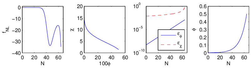
The time evolution of from the formula is given in Fig. 4, where the final point is identified as some time during inflation. This method is also used in Vernizzi and Wands [20] for analytic evolution. We can see that increases sharply around . This can be understood from the evolution of two fields: from this time, the velocity of (or ) increases (as seen in the third and fourth plot of Fig. 4) to satisfy the condition Eqn. (36) to obtain large non-Gaussianity. Then begins to decrease around as becomes bigger than . Note that, around the region for large , the curvature perturbation of -field becomes comparable to, and then dominates, that of the -field. Around , the -field begins to roll so fast that decreases and increases once more. However during this fast-roll stage, slow-roll breaks down and our analytic formula is not valid any more. Thus we calculate final values when .
We note, for reference, that in this regime of large non-Gaussianity, the background trajectory must be at almost entirely in the one-field direction. We therefore expect reheating to take place in almost the same way as it would in normal chaotic inflation.
V.2 Quadratic product potential
In this section we show that a direct coupling between and , leaving to the product potential
| (64) |
cannot generate a large non-Gaussianity during inflation. From the equation it follows that the fields evolve according to
| (65) |
and similarly for . Hence we have in Region B, where and ,
| (66) |
Hence decreases during inflation and this model cannot generate .
V.3 Hybrid inflation
We consider a model of 2 field hybrid inflation,
| (67) |
which is vacuum dominated, i.e. which satisfies and . Here we assume that inflation ends abruptly by another waterfall field which we don’t write down in the potential above. We note that may change depending on the details of how the waterfall field is coupled to the two inflaton fields [15, 16, 18], but in general this is unlikely to generate a large contribution to without fine-tuning [17].
In this regime the slow-roll solutions are [5], (we can identify and in the notation of that paper)
| (68) |
and the slow-roll parameters are
| (69) |
We note that the dominant slow-roll parameters and are constant in this model.
For this case, since , from Eqn. (54) (or equivalently Eqn. (55)) in Region D, where and , it follows that
| (70) |
In the above we have used Eqn. (51) for in Region D. We hence require the condition, Eqn. (57),
| (71) |
and find the exact upper limits on the parameters:
| (72) |
Noting that in Region D , from Eqn. (68) we require so that grows significantly during inflation.
In Table 1, we give some explicit examples of values of and which lead to a large non-Gaussianity. Using Eqn. (43) we also calculate the spectral index. The contours of of this sum potential for a specific choice of and is given in Fig. 5 The first example in the Table 1 shows that it is possible to have and a scale invariant spectrum. The tensor-to-scalar ratio is also small in this example.
| r | ||||||
|---|---|---|---|---|---|---|
| 0.018 | -0.018 | 1 | 0.00018 | -42 | 0 | 0.006 |
| 0.04 | 0.005 | 1 | 0.0018 | 9.27 | 0.09 | 0.10 |
| 0.01 | -0.02 | 1 | 0.00037 | -11.1 | -0.02 | 0.026 |

Our formula for is also consistent with the calculation of [5] but our analysis of the parameter space is more extensive and in particular it allows for very small initial field values. We therefore find a region with much larger non-Gaussianity than was found in [5].
As a further check on the algebra, we note that it is also possible to analyse this model using the formalism of a product potential with . This is equivalent to the sum potential Eqn. (67) in the limit of vacuum domination ( and ). We have checked that this gives the same results. We note from Table 1 that we require a very small value of in Region D. If the value becomes too small then the motion of the field will become dominated by quantum fluctuations rather than the classical drift down the potential, , which we have assumed. In order that we can neglect the effect of the quantum fluctuations, the condition we require on the background trajectory is [40]. Using , and Eqn. (42) the condition that the classical trajectory is valid can be rewritten as , where . We have checked that this is satisfied for all of the examples given in the Table 1, but it does provide a significant constraint on the total parameter space.
Very recently Cogollo et al. have calculated the effect of the loop correction to the primordial power spectrum and bispectrum [41]. This loop correction arises from taking into account the contribution to the power spectrum and bispectrum arising from terms in the expansion which are non-leading in the expansion of the field perturbation , see e.g. [42]. However they can still be significant if the coefficient to the term given by the derivative of is extremely large, e.g. [43]. These “higher order” terms are usually neglected, but [41] has shown the first explicit example of an inflation model where they cannot be neglected. They consider a 2-field hybrid model with the same potential as Eqn. (67) in the special case of an unstable straight trajectory along one of the axes, with and both negative. In this case, they find (for certain initial values) the loop correction is dominant and can generate an observable . We have checked that for the explicit values given in the table the loop correction does not dominate (under the assumption that the same loop correction is dominant here as the one in [41]). However this does provide a further restriction on the allowed parameter space of the “tree level” calculation of the model, which is assumed in Eqn. (70). We plan to return to this issue, and make a more thorough investigation of the hybrid model in a future publication.
VI Non-Gaussianity with Non-Canonical Kinetic Terms (Product Potentials)
Generally, the scalar fields need not only couple through the potential, but may also couple kinetically [44, 45, 46, 47]. In this section, therefore, we consider inflation governed by the following generalised action:
| (73) |
When the kinetic energies are non-canonical, the local non-Gaussianity is altered from the previous sections. In the case of the sum potential, the modifications are non-trivial and are difficult to analyse. When the potential is of product form, however, we may at least partially use the previous analysis. We therefore concentrate only on a product potential, but our findings relate also to sum potentials.
Using new auxiliary functions, Eqn. (74) can be re-written as:
| (78) | |||||
where
| (79) |
If , then and , , and . The function is plotted for various values of in Figs. 6. From this definition, it is clear that allowing , the range of for which we can obtain large opens up. We also note that the symmetry between two fields is broken, due to , which is apparent in Figs. 6. Note, though, that we require as before. Furthermore, when (or ), we no longer require .
Expressions for the power spectra and spectral index with a non canonical kinetic term are given in [21, 47].

VII Conclusion
We have made an in depth investigation into the level of non-Gaussianity during two-field slow-roll inflation. We have shown that it is possible to generate a large level of non-Gaussianity during inflation without violating slow roll and when the inflaton field perturbations are Gaussian at Hubble exit.
The general conditions for generating a large non-Gaussianity show that the inflaton potential must have a specific shape so that the angle of the background trajectory can grow by about two orders of magnitude or more during inflation. In the case of an inflation potential made of a product of two quadratic potentials, this condition is not possible so that we conclude this model cannot generate a large non-Gaussianity during slow roll inflation. When the angle of the background trajectory grows sufficiently (in relative terms), we still need one of the fields to dominate throughout inflation, yet the remaining field can not remain full insignificant. For typical values of the slow roll parameters, we require that initially the subdominant field, say , must satisfy . This means that the field trajectory is almost exactly parallel to the axes initially and typically this requires a finely tuned initial condition. In the case of a product separable potential we then also require that the final value of the angle of the background trajectory lies in a narrow range much greater than the initial value (in relative terms) but still nearly parallel to the axis. The analysis for a sum separable potential is very similar but more complicated to analyse. The initial background trajectory must be similarly fine-tuned to be nearly parallel to one of the axes of the inflaton fields, but the tuning at the end of inflation is not written so simply. We have also shown how the constraints on generating a large non-Gaussianity may be eased if we generalise the inflaton model to allow a non-canonical kinetic term.
We have presented two explicit models where a large non-Gaussianity can be generated during slow roll inflation. One is a product potential driven by a field with a quadratic potential, which ends inflation when it approaches the minimum of the potential. If the second field with an exponential potential has a sufficiently small initial value then for certain values of the model parameter, , this field grows by the right amount to generate a large non-Gaussianity, . We also consider the sum separable model of hybrid inflation. We provide a few specific choices of the model parameters, which are effectively and , for a suitably large ratio of the initial field values this model generates a large non-Gaussianity. We find this is possible either if the ’s have the opposite sign (so that inflation takes place near a saddle point) or when both of the ’s have the same sign. However we have also found that if one of the field values is too small then quantum fluctuations may perturb the background trajectory to an extent that the classical trajectory in field space is no longer valid. There is also the possibility that the large scale loop correction which we have not generally considered in this paper may not be negligible. We intend to return to these issues and make a more thorough investigation of the hybrid model in a future publication.
Acknowledgements.
The authors thank Carsten van de Bruck, Filippo Vernizzi and David Wands for useful comments. CB acknowledges financial support from the Deutsche Forschungsgemeinschaft. K.-Y.C. is supported by the Ministerio de Educacion y Ciencia of Spain under Proyecto Nacional FPA2006-05423 and by the Comunidad de Madrid under Proyecto HEPHACOS, Ayudas de I+D S-0505/ESP-0346. LMHH acknowledges support from STFC.References
- [1] J. M. Maldacena, JHEP 0305, 013 (2003) [arXiv:astro-ph/0210603].
- [2] N. Bartolo, E. Komatsu, S. Matarrese and A. Riotto, Phys. Rept. 402 (2004) 103 [arXiv:astro-ph/0406398].
- [3] D. Seery and J. E. Lidsey, JCAP 0509, 011 (2005) [arXiv:astro-ph/0506056].
- [4] N. Bartolo, S. Matarrese and A. Riotto, Phys. Rev. D 65 (2002) 103505 [arXiv:hep-ph/0112261].
- [5] L. Alabidi, JCAP 0610 (2006) 015 [arXiv:astro-ph/0604611].
- [6] K. Enqvist, A. Jokinen, A. Mazumdar, T. Multamaki and A. Vaihkonen, Phys. Rev. Lett. 94 (2005) 161301 [arXiv:astro-ph/0411394].
- [7] A. Jokinen and A. Mazumdar, JCAP 0604 (2006) 003 [arXiv:astro-ph/0512368].
- [8] X. Chen, M. x. Huang, S. Kachru and G. Shiu, JCAP 0701 (2007) 002 [arXiv:hep-th/0605045].
- [9] N. Barnaby and J. M. Cline, Phys. Rev. D 73, 106012 (2006) [arXiv:astro-ph/0601481].
- [10] A. Misra and P. Shukla, arXiv:0807.0996 [hep-th].
- [11] X. Chen, R. Easther and E. A. Lim, JCAP 0706, 023 (2007) [arXiv:astro-ph/0611645].
- [12] E. Silverstein and D. Tong, Phys. Rev. D 70, 103505 (2004) [arXiv:hep-th/0310221]; M. Alishahiha, E. Silverstein and D. Tong, Phys. Rev. D 70, 123505 (2004) [arXiv:hep-th/0404084]; M. x. Huang and G. Shiu, Phys. Rev. D 74, 121301 (2006) [arXiv:hep-th/0610235].
- [13] S. Mollerach, Phys. Rev. D 42 (1990) 313; A. D. Linde and V. F. Mukhanov, Phys. Rev. D 56, 535 (1997) [arXiv:astro-ph/9610219]; K. Enqvist and M. S. Sloth, Nucl. Phys. B 626, 395 (2002) [arXiv:hep-ph/0109214]; D. H. Lyth and D. Wands, Phys. Lett. B 524, 5 (2002) [arXiv:hep-ph/0110002]; T. Moroi and T. Takahashi, Phys. Lett. B 522, 215 (2001) [Erratum-ibid. B 539, 303 (2002)] [arXiv:hep-ph/0110096]; K. Enqvist and S. Nurmi, JCAP 0510, 013 (2005) [arXiv:astro-ph/0508573]; A. Linde and V. Mukhanov, JCAP 0604, 009 (2006) [arXiv:astro-ph/0511736]; K. A. Malik and D. H. Lyth, JCAP 0609, 008 (2006) [arXiv:astro-ph/0604387]; M. Sasaki, J. Valiviita and D. Wands, Phys. Rev. D 74, 103003 (2006) [arXiv:astro-ph/0607627].
- [14] T. Suyama and M. Yamaguchi, Phys. Rev. D 77, 023505 (2008) [arXiv:0709.2545 [astro-ph]]; L. Kofman, arXiv:astro-ph/0303614; G. Dvali, A. Gruzinov and M. Zaldarriaga, Phys. Rev. D 69, 023505 (2004) [arXiv:astro-ph/0303591].
- [15] F. Bernardeau and J. P. Uzan, Phys. Rev. D 67, 121301 (2003) [arXiv:astro-ph/0209330].
- [16] D. H. Lyth, JCAP 0511, 006 (2005) [arXiv:astro-ph/0510443]; M. P. Salem, Phys. Rev. D 72, 123516 (2005) [arXiv:astro-ph/0511146].
- [17] L. Alabidi and D. Lyth, JCAP 0608, 006 (2006) [arXiv:astro-ph/0604569].
- [18] M. Sasaki, Prog. Theor. Phys. 120 (2008) 159 [arXiv:0805.0974 [astro-ph]]; A. Naruko and M. Sasaki, arXiv:0807.0180 [astro-ph].
- [19] B. Dutta, L. Leblond and J. Kumar, arXiv:0805.1229 [hep-th].
- [20] F. Vernizzi and D. Wands, JCAP 0605, 019 (2006) [arXiv:astro-ph/0603799].
- [21] K. Y. Choi, L. M. H. Hall and C. van de Bruck, JCAP 0702 (2007) 029 [arXiv:astro-ph/0701247].
- [22] T. Battefeld and R. Easther, JCAP 0703, 020 (2007) [arXiv:astro-ph/0610296].
- [23] D. Seery and J. E. Lidsey, JCAP 0701, 008 (2007) [arXiv:astro-ph/0611034].
- [24] G. I. Rigopoulos, E. P. S. Shellard and B. J. W. van Tent, Phys. Rev. D 76, 083512 (2007) [arXiv:astro-ph/0511041].
- [25] S. Yokoyama, T. Suyama and T. Tanaka, Phys. Rev. D 77, 083511 (2008) [arXiv:0705.3178 [astro-ph]]; S. Yokoyama, T. Suyama and T. Tanaka, Phys. Rev. D 77 (2008) 083511 [arXiv:0711.2920 [astro-ph]].
- [26] C. Gordon, D. Wands, B. A. Bassett and R. Maartens, Phys. Rev. D 63, 023506 (2001) [arXiv:astro-ph/0009131].
- [27] A. A. Starobinsky, JETP Lett. 42, 152 (1985) [Pisma Zh. Eksp. Teor. Fiz. 42, 124 (1985)].
- [28] M. Sasaki and E. D. Stewart, Prog. Theor. Phys. 95 (1996) 71 [arXiv:astro-ph/9507001].
- [29] M. Sasaki and T. Tanaka, Prog. Theor. Phys. 99, 763 (1998) [arXiv:gr-qc/9801017].
- [30] D. H. Lyth, K. A. Malik and M. Sasaki, JCAP 0505, 004 (2005) [arXiv:astro-ph/0411220].
- [31] D. H. Lyth and Y. Rodriguez, Phys. Rev. Lett. 95 (2005) 121302 [arXiv:astro-ph/0504045].
- [32] D. Wands, N. Bartolo, S. Matarrese and A. Riotto, Phys. Rev. D 66, 043520 (2002) [arXiv:astro-ph/0205253].
- [33] D. H. Lyth and I. Zaballa, JCAP 0510, 005 (2005) [arXiv:astro-ph/0507608].
- [34] E. Komatsu and D. N. Spergel, Phys. Rev. D 63, 063002 (2001) [arXiv:astro-ph/0005036].
- [35] E. Komatsu et al. [WMAP Collaboration], arXiv:0803.0547 [astro-ph].
- [36] C. T. Byrnes, M. Sasaki and D. Wands, Phys. Rev. D 74, 123519 (2006) [arXiv:astro-ph/0611075].
- [37] http://www.rssd.esa.int/index.php?project=Planck
- [38] L. Kofman, A. D. Linde and A. A. Starobinsky, Phys. Rev. Lett. 73 (1994) 3195 [arXiv:hep-th/9405187].
- [39] L. Kofman, A. D. Linde and A. A. Starobinsky, Phys. Rev. D 56 (1997) 3258 [arXiv:hep-ph/9704452].
- [40] P. Creminelli, S. Dubovsky, A. Nicolis, L. Senatore and M. Zaldarriaga, JHEP 0809 (2008) 036 [arXiv:0802.1067 [hep-th]].
- [41] H. R. S. Cogollo, Y. Rodriguez and C. A. Valenzuela-Toledo, JCAP 0808 (2008) 029 [arXiv:0806.1546 [astro-ph]].
- [42] C. T. Byrnes, K. Koyama, M. Sasaki and D. Wands, JCAP 0711, 027 (2007) [arXiv:0705.4096 [hep-th]].
- [43] L. Boubekeur and D. H. Lyth, Phys. Rev. D 73, 021301 (2006) [arXiv:astro-ph/0504046].
- [44] J. Garcia-Bellido and D. Wands, Phys. Rev. D 52 (1995) 6739 [arXiv:gr-qc/9506050].
- [45] J. Garcia-Bellido and D. Wands, Phys. Rev. D 53 (1996) 5437 [arXiv:astro-ph/9511029].
- [46] A. A. Starobinsky, S. Tsujikawa and J. Yokoyama, Nucl. Phys. B 610 (2001) 383 [arXiv:astro-ph/0107555].
- [47] F. Di Marco, F. Finelli and R. Brandenberger, Phys. Rev. D 67 (2003) 063512 [arXiv:astro-ph/0211276]; F. Di Marco and F. Finelli, Phys. Rev. D 71 (2005) 123502 [arXiv:astro-ph/0505198].