Particle Multiplicity in Jets and Sub-jets with Jet Axis from Color Current
Wolfgang Ochs11 1 E-mail: wwo@mppmu.mpg.de
Max-Planck Institut für Physik, Werner-Heinsenberg-Institut
Föringer Ring 6, D-80805 München, Germany
Redamy Pérez Ramos22 2 E-mail: redamy@mail.desy.de
II. Institut für Theoretische Physik, Universität Hamburg
Luruper Chaussee 149, D-22761 Hamburg, Germany
Abstract: We study the particle multiplicity in a jet or sub-jet as derived from an energy-multiplicity 2-particle correlation. This definition avoids the notion of a globally fixed jet axis and allows for the study of smaller jet cone openings in a more stable way. The results are sensitive to the mean color current in the jet from primary parton which takes into account intermediate partonic processes in the sub-jet production where at high energies. We generalize previous calculations in Leading Logarithmic Approximation (LLA). The size of the effects related to this jet axis definition are computed for multiplicities in sub-jets with different opening angles and energies by including contributions from the Modified LLA (MLLA) and Next-to-MLLA to the leading order QCD results.
Keywords: perturbative Quantum Chromodynamics, jets, multiplicity
1 Introduction
The collimation of hadrons in jets is a basic phenomenon of high energy collisions and its quantitative understanding is an important task for QCD. Simple differential characteristics of a jet are their energy and multiplicity angular profiles. The collimation of energy and multiplicity in the jet follows from the dominance of gluon bremsstrahlung processes in the parton cascade evolution. Whereas the former is more sensitive to the hard processes inside a jet the second one is sensitive to the soft parton emissions from the primary parton.
The characteristics of soft particle production, such as particle multiplicities, inclusive distributions and correlation functions, are derived in QCD in the Modified Leading Logarithmic Approximation (MLLA) (for review, see [1]) which takes into account the leading double logarithmic terms and the single logarithmic corrections. These azimuthally averaged quantities can be obtained from an evolution equation for the generating functional of the parton cascade. This equation provides also Next-to-MLLA corrections taking into account energy conservation of parton splittings with increased accuracy. The corresponding hadronic observables can be obtained using the concept of Local Parton Hadron Duality (LPHD) [2] which has turned out a successful description of many hadronic phenomena (see, e.g. [3]).
A characteristic prediction of QCD is the increased mean particle multiplicity in a gluon jet over the quark jet, asymptotically by the ratio of color factors modified by corrections in powers of [4, 5, 6]. These results have been compared with LEP data on 2- and 3-jet events, interpreted as and primary production [7, 8, 9]. In applications with primary hadron beams, such as at HERA, RHIC, TEVATRON or LHC it is necessary to select jets by an angular cut to remove the effects from the hadron remnants. Such an analysis of multiplicities has been performed at the TEVATRON [10] with different jet opening angles and energies . The multiplicity as well as differential multiplicity distributions in MLLA depend on the maximum transverse momentum in the jet (“virtuality”), i.e. on the combination
| (1) |
in the small angle approximation. This scaling behavior has been verified [10] for the multiplicities in the angular range and also for the peak position of the inclusive rapidity spectra [11]. Results from LEP and TEVATRON support in general the theoretical treatment based on the MLLA evolution equation and the agreement with data improves with the inclusion of higher order terms in .
For small opening angles the definition of the jet axis becomes problematic because of the fluctuations at low particle multiplicity. The multiplicity at smaller angles can be defined in a more stable way without reference to a jet axis by the double inclusive correlation density between two particles. The particles (p2) within the cone around particle (p1) are counted with angle (including particle (p1) itself), then the superposition of the particles (p1) in the jet weighted by their energies is performed. For a jet of full energy , in a form differential in the energy fraction , the multiplicity in the cone is given as (see Ref. [1])
| (2) |
In this definition, the collection of particles (p1) serves to replace the jet axis and therefore, also small angles are well defined, which is not the case for the usual global jet axis definition.
The evaluation of Eq. (2) for the distribution in energy and, after integration, for the multiplicity of particles (p2) in the cone has been obtained in LLA for the integral over the energy in Refs. [12, 1]. The definition of jet axis is especially relevant for the inclusive distribution of the transverse momentum of particles and this quantity has been derived with reference to the energy flux in the MLLA [13] and including an important class of Next-to-MLLA (NMLLA) contributions as obtained from the evolution equation [14]. The predictions on the distributions have been found in a rather good agreement with the preliminary data ( GeV) from the CDF collaboration [15] using so far a conventional jet definition. In this paper we study the effects from the definition Eq. (2) and derive results for particles confined into small cones. This allows the study of particle distributions with smaller in the jet and lower effective energies (virtuality) than the nominal jet energy .
For decreasing cone size of a sub-jet in the definition of Eq. (2) the simple scaling behavior as in Eq. (1) will be broken. The occurrence of intermediate processes leads to a mixing of quark and gluon sources and, asymptotically in the LLA, the hadron multiplicity in the sub-jet with opening angle in the primary jet from parton ( or ) and large opening angle is given by [1]
| (3) |
proportional to the multiplicity of an isolated gluon jet of virtuality . The average color current inside the small cone is obtained in the same approximation [1] as
| (4) |
where denotes the mean energy fraction of parton inside parton jet for given jet virtualities and . This quantity is found in between the color factors
| (5) |
The hadron multiplicity , as suggested by LPHD, is taken proportional to the parton multiplicity at cut-off scale , i.e. with hadronization constant .
Using the alternative approach for jet definition from Eq. (2) we derive in this paper results on the particle multiplicity as a simple observable showing its dependence on the color current and its variation with jet energy and opening angle in the improved accuracy of MLLA and NMLLA. Some phenomenological applications will be studied.
2 Evolution equations for multiplicities in quark and gluon jets
In MLLA the evolution of azimuthally averaged quantities with jet energy and jet opening is given by an evolution equation for the generating functional for the parton momenta in the jet [1]. The evolution involves , the running coupling constant of QCD
| (6) |
where is the intrinsic scale of QCD and is the first term in the perturbative expansion of the function 33 3 Following common practice, we consider in this work on soft particles the 1-loop expression for the running coupling constant, therefore has to be considered a phenomenological parameter not related to the usual . , is the number of colors, , where is the number of light quark flavors. In Double Logarithmic Approximation (DLA) is also linked with the anomalous dimension of twist-2 operators by
| (7) |
where is the collinear cut-off parameter for . The results depend on energy and angle only through the variable , i.e. the maximum transverse momentum in the jet. We also set in the following.
For the evolution of the mean multiplicities in quark and gluon jets one obtains in MLLA the coupled system of two evolution equations [1]
| (8) | |||||
Together with initial conditions for the multiplicities at threshold (every jet contains only one parton, quark or gluon) these equations determine the multiplicities at the higher values of . The DGLAP splitting functions denoted by are given by
The equations above for multiplicities can be solved analytically [9] in terms of an expansion in of the ratio of multiplicities and the QCD anomalous dimension defined by
| (9) |
The Eqs. (8) are complete only up to MLLA order. The emerging higher order terms in the asymptotic expansion, although not complete, provide, however, an important contribution improving the constraint from energy conservation. In particular, they build the correct threshold behavior of the parton cascade and therefore a better behavior at the present energies is obtained. A full numerical solution of the evolution equation [16] corresponding to an all order resummation has in fact provided a rather close reproduction of the multiplicity ratio above; the same is also true for the result of the HERWIG MC [17] at parton level and at hadron level. On the other hand, the truncated series in while asymptotically convergent, diverges at low energies.
We limit ourselves here to the NMLLA expression of that reads
| (10) |
where the asymptotic value of is . The MLLA term has been calculated in [4]. The coefficients can be obtained from the Taylor expansions of and for and respectively and from equating the terms of the same order in in both sides of Eq. (8); the values for for NMLLA read and [9]. The NMLLA solution for the mean multiplicity in a gluon jet is found as [9]
| (11) |
with , at ; is the LPHD normalization factor. The pre-exponential term is the MLLA contribution to , while the one , the NMLLA one. We give accordingly, the expressions of the first and second logarithmic derivatives of that follow from Eq. (11)
| (12) |
| (13) |
which we will all use in the following. The NMLLA solution for can be obtained by substituting Eq. (11) into Eq. (10).
3 Energy-multiplicity correlations
We consider the production of a jet in a high energy collision (, , , …) initiated from a parton of energy and with opening angle which separates it from other jets.
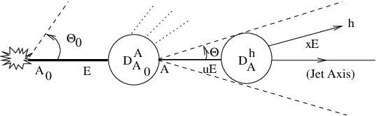
A sub-jet is defined by the opening angle with respect to parton with momentum fraction . The distribution of the momentum fraction of a hadron in this sub-jet is obtained by the integration of the double-inclusive correlation function in Eq. 2, see Ref. [12]. This process is depicted in Fig. 1. Notations and kinematics are identical to the ones used in the work of Ref. [13] which also contains further details.
The distribution is obtained as the convolution of two fragmentation functions [1]
| (14) |
This equation expresses the correlation between the energy flux and one particle () within the sub-jet with angle generated from intermediate parton and with energy fraction . The function in (14) describes the probability to emit parton of virtuality with energy fraction off the initial parton ( or ), taking into account the evolution of the jet between and . The function in Eq. (14) describes the probability to produce the hadron off with energy fraction and transverse momentum scale .
Integrating (14) over the energy fraction yields the corresponding sub-jet multiplicity of hadrons inside the angular range of the jet
| (15) |
where is the number of hadrons (partons at scale ) produced inside the sub-jet of total virtuality .
We also note two limits of the sub-jet multiplicity in Eq. (15). At first, in the limit of large angle one finds, see also [1],
| (16) |
and the sub-jet multiplicity coincides with the overall jet multiplicity. At small opening angle
| (17) |
the sub-jet multiplicity approaches the limit of one particle. This limit cannot be reached in our approximation with a truncated expansion in .
3.1 Approximations with the leading parton
The convolution integral in Eq. (15) is dominated by the region as is exponentially rising with and the behavior leads to a slowly varying function (for further discussion, see [13]). Therefore, we use the DGLAP expressions for in the following, then the evolution between the two scales depends only on the variable
| (18) |
and for we also write for short.
Within the leading parton approximation we expand the multiplicity in (15) at . As in the MLLA evolution equation (8) and thereafter we take a logarithmic dependence of multiplicity and for and for , this quantity can be written as
| (19) |
up to the NMLLA level of accuracy. Therefore, in this approximation the correlation integral in (15) can be replaced by a sequence of factorized terms showing alternating sign
| (20) |
Here depends only on and the mean energy fraction is given by
| (21) |
where is the representation of DGLAP fragmentation functions in Mellin’s space [1]
| (22) |
The other moments can be obtained by differentiation after the exponent
| (23) |
The lower bound in Eqs. (22) and (23) has been set to in the limit , as the threshold region in the integral Eq. (15) is exponentially suppressed. The second term in Eq. (21) follows from the scaling violation in DGLAP fragmentation functions when one sets in the third argument of in Eq. (15); it has been proved in App. D of [14] not to exceed of the leading contribution, that is why we neglect it hereafter and simply set as in [1, 14].
Now Eq. (20) can be conveniently rewritten in the form
| (24) | |||||
and, using Eqs. (12) and (13), we obtain an expansion in
| (25) | |||||
where the contribution is the leading one (LLA) determined in [1]
| (26) | |||||
| (27) |
with , , , where and . The functions and are determined from (23), as in [13]. Taking and at their QCD values the results still depend on . As this dependence is rather weak, we present the results with numerical coefficients only for in the appendix. In the limit the expression in Eq. (25) fulfills the limit Eq. (16) as the mean values in Eq. (23) vanish and .
3.2 Multiplicity and color current
The expression for can be written in compact form as in Eq. (3) introducing the color current. In the sum over in Eq. (25) when is a quark () we replace
| (28) |
according to Eq. (10) and after multiplication with the terms inside the square bracket we keep only terms up to so as to respect the NMLLA scheme . One thus obtains the average multiplicity of soft hadrons within sub-jet angle with respect to the energy flow in terms of the gluon jet multiplicity
| (29) |
where is given by the solution Eq. (11) of the evolution equation (8) and ( is the average color current of partons forming the energy flux
| (30) | |||||
These color currents are also presented in the appendix with numerical coefficients for (see Eqs. (40) and (41)). The ratio of the gluon to the quark jet average multiplicity reads
| (31) |
For this quantity in the limit (), the appropriate ratio ) is recovered.


The color currents inside gluon and quark jets and are displayed in Fig. 2 for a particular jet virtuality GeV in the LLA, MLLA and NMLLA. For simplicity we also use () which is known to be a good approximation for hadron spectra (“limiting spectrum”). As expected from Eqs. (30) and (40), for , all curves for coincide at , where is the color factor corresponding to the splitting of one gluon (in this case the one initiating the jet) into two other gluons. In the same limit , the color current in LLA approaches , where is the color factor corresponding to the splitting of a quark into a quark and a gluon. The mismatch at between the MLLA and the LLA curves comes from the -expansion of and equals , while the difference between the LLA curve and the NMLLA curve is increased by the correction and reaches ).
The role of and corrections to the LLA color current in Eq. (30) is quite important and the expansion in is seen in Fig. 2 to oscillate if higher order terms are incorporated. Indeed, the terms change sign as one goes from the LLA () to MLLA () and to the NMLLA (). Because of the running coupling the -expansion () converges at high energies but may diverge at low energies. At present energies ( at LEP) the expansion is converging rather slowly and one may ask for yet higher order terms. Such calculations would also require higher order terms in the expansion of the ratio and its derivatives which are not available. As an exercise, we calculated 6 terms beyond LLA for the gluon current numerically while keeping the expansion of at second order in . Then the solutions keep oscillating with a new solution falling in between the two previous ones. The trend is towards a solution closer to NMLLA than to MLLA.
Starting with the isolated jet at the sub-jets at smaller angles may evolve from intermediate partons of different color. Therefore, one expects that sub-jets in a gluon jet have lower multiplicity than isolated gluon jets at the same angle () and the opposite for a quark jet. This behavior is in fact born out by the MLLA and NMLLA curves for which show the same trends as the LLA term: it is increasing with at the higher energies. On the other hand, the quark color current is decreasing in LLA and in the NMLLA while for the intermediate approximation MLLA this behavior is not yet reached. Asymptotically () all curves have to approach either or .
3.3 Results on multiplicities at small angles


Next we study the consequences for the behavior of multiplicities at full angles and for sub-jets at reduced angles . Results for multiplicities using our formulae for color currents Eqs. (29) and (30) are shown in Figs. 3 and 4 for MLLA (left panels) and NMLLA (right panels). The full lines show the particle multiplicity for an isolated jet as function of , i.e. as function of the jet energy for the gluon jet in Fig. 3 and for the quark jet in Fig. 4, according to Eqs. (9) and (11). The hadronization constant has been taken as according to [9].


Also shown in these figures are the multiplicities for the reduced opening angle as function of for different fixed energies but variable sub-jet angles . For these curves approach the full multiplicities at . In the simple model with the scaling of multiplicities with in Eq. (1) all these curves would coincide; the existence of intermediate processes and non-trivial color currents yields the predicted scale breaking. The mixing of quark and gluon jets will reduce the multiplicity in the gluon jet and increase it in the quark jet at sufficiently high energies. This property is reproduced in our calculations except for in MLLA where the appropriate high energy regime is not yet reached.
In case of the ratio the effects from gluon and quark jets go in the same direction and yield the observable scale breaking effects of Fig. 5 for the small cone measurements. For the LEP energy range () the ratio for large jet opening angle is in MLLA and in NMLLA. This is still larger than the experimentally observed [7, 8] which indicates the slow convergence of the expansion of multiplicity. As emphasized in Sect. 2 the numerical treatment of the evolution equation removes this discrepancies largely. The effect from intermediate processes in the new definition of multiplicity amounts to about 20% in NMLLA at a reduced energy scale .
4 Conclusions
We have studied a definition of jet axis which is based on a 2-particle correlation where the jet axis corresponds to the energy weighted direction of particles in a given cone . In this way smaller angles (or transverse momenta) can be meaningfully determined. We studied especially the effects related to a measurement of multiplicities where we have added MLLA and NMLLA corrections to the known LLA results and studied phenomenological consequences numerically.
The main new effect from 2-particle correlations is the appearance of the “color current” in the result which reflects the possibility of intermediate quark-gluon processes. This effect can be seen by the scale breaking between jets and sub-jets at the same scale but different energies and opening angles . Typical effects are of the order of 20%.
The expansion in which is used in the calculation of color currents is rather slowly converging and MLLA in the considered energy range is not satisfactory whereas NMLLA shows the expected behavior at the qualitative level. For a more quantitative treatment higher order terms have to be calculated but this requires also a treatment of the multiplicity ratio at higher orders which is not yet available. Alternatively, numerical methods and Monte Carlo calculations may be accessible.
As an interesting application, one could learn from a single type of jet about properties of the other type by the study of sub-jets of lower energies (for example, from a high energy gluon jet at LHC about quark jets of lower energies). Other applications concern behavior of spectra at small transverse momenta or low energy gluon jets.
Appendix: Expressions for , and the color currents
Setting we obtain the MLLA correction from Eq. (23) for and
| (32) |
| (33) |
| (34) |
| (35) |
for the NMLLA correction with we also write the result for
| (36) | |||||
| (37) | |||||
| (38) | |||||
| (39) | |||||
Substituting the former results in (30) and setting
yields the color currents, evaluated again for ,
| (40) | |||||
| (41) | |||||
References
- [1] Yu.L. Dokshitzer, V.A. Khoze, A.H. Mueller & S.I. Troyan, Basics of Perturbative QCD, Editions Frontières, Paris (1991).
- [2] Ya.I. Azimov, Yu.L. Dokshitzer, V.A. Khoze & S.I. Troian, Z. Phys. C 27 (1985) 65. Yu.L. Dokshitzer, V.A. Khoze & S.I. Troian, J. Phys. G 17 (1991) 1585.
- [3] V.A. Khoze & W. Ochs; Int. J. Mod. Phys. A 12 (1997) 2949.
- [4] A.H. Mueller, Nucl. Phys. B 241 (1984) 141; Erratum ibid., B 241 (1984) 141.
- [5] E.D. Malaza & B.R. Webber, Phys. Lett. B 149 (1984) 501.
- [6] I.M. Dremin, V.A. Nechitailo, Mod. Phys. Lett. A 9 (1994) 1471; JETP Lett. 58 (1993) 945.
- [7] G. Abbiendi et al., [OPAL Collaboration], Phys. Rev. D 69 (2004) 032002.
- [8] J. Abdallah et al. [DELPHI Collaboration], Eur. Phys. J. C 44 (2005) 311.
- [9] I.M. Dremin & J.W. Gary, Phys. Rep. 349 (2001) 301.
- [10] D. Acosta et al., Phys. Rev. Lett. 94 171802 (2005).
- [11] A.N. Safonov (for CDF Collaboration), Nucl. Phys. B (Proc. suppl.) 86 (2000) 55.
- [12] Yu.L. Dokshitzer, D.I. Dyakonov & S.I. Troyan, Phys. Rep. 58 (1980) 270.
- [13] R. Perez-Ramos & B. Machet, JHEP 04 (2006) 043.
- [14] R. Perez-Ramos, F. Arléo & B. Machet, arXiv:0712.2212 [hep-ph], Phys. Rev. D in press; F. Arléo, R. Perez-Ramos & B. Machet, Phys. Rev. Lett. 100 (2008) 052002 .
- [15] S. Jindariani, A. Korytov & A. Pronko: “ Distributions of Particles in Jets at CDF”, CDF report CDF/ANAL/JET/PUBLIC/8406 (March 2007), www-cdf.fnal.gov/physics/new/qcd/ktdistributions_06/cdf8406_Kt_jets_public.ps
- [16] S. Lupia & W. Ochs, Phys. Lett. B 418 (1998) 214.
- [17] G. Corcella et al., JHEP 01 (2001) 010.