Lower bounds on dissipation upon coarse graining
Abstract
By different coarse-graining procedures we derive lower bounds on the total mean work dissipated in Brownian systems driven out of equilibrium. With several analytically solvable examples we illustrate how, when and where the information on the dissipation is captured.
pacs
05.70.Ln, 05.40.-aI Introduction
Equilibrium statistical physics provides the microscopic foundation of thermodynamics, built around the concept of entropy as the logarithm of the phase volume. The theory has been extended to the regime of linear irreversible thermodynamics by identifying the entropy production in the regime of linear response [1, 2, 3, 4]. There exists to date no general theory covering far from equilibrium situations. However, recent results known as fluctuation [5, 6, 7, 8, 9] or work [10, 11, 12, 13, 14, 15, 16, 17, 18] theorems point to the existence of exact equalities valid independent of the distance from equilibrium. These equalities involve fluctuations in work or entropy production. For the average of these quantities, they reduce to inequalities, in agreement with the second law of thermodynamics. For example, the Jarzynski equality states that , where is the work needed to bring a system, in contact with a heat bath at temperature () from one initial equilibrium state to a final one, and is the difference in free energy of these states (see [14] for a more precise discussion). Then by the application of Jensen’s inequality one finds . While the work and fluctuation theorems are certainly intriguing results of specific interest for the study of small systems, they provide no extra information on the average value of work and entropy production.
Parallel to these developments, the direct calculation of work, entropy and dissipation has proceeded following various channels of research. Explicit results for path dependent dissipation or entropy production have been obtained, mostly in the context of Markovian stochastic models [19, 20, 21, 22]. The average entropy production goes back to earlier work [24, 23]. Recently the microscopically exact value of the average dissipated work has been obtained in a set-up similar to that of the work theorem [25]. The connection and consistency between this exact Hamiltonian result and the ones derived in the context of stochastic models has been clarified in [26].
The main issue of this paper is to discuss how this type of formulas can be applied when only limited information on the system is available. In other words how much of the irreversible behavior is revealed when only partial measurements are performed. Complimentary to this issue is the identification of the variables in which the traces of the dissipation reside. One could imagine that such knowledge would allow to develop mechanisms to either increase or decrease the dissipation. The limitations in observation can be of different nature. It could be that the monitoring in time is not exhaustive, but one only performs a finite number of punctual measurements. The measurement of the variables could also be crude or incomplete. Or both limitations could be present. We will show that this limited information provides a lower bound for the dissipation. Of particular interest is to know whether this bound is close to the full dissipation or just reproduces the general bound that is contained in the second law. As such, the analysis will reveal when and where the information on the dissipative process is located. For our illustration, we will focus on systems described by stochastic dynamics. The latter provide an accurate description of mesoscopic phenomena in physics, chemistry and biology, and have been used extensively especially in the context of Brownian entities appearing in nano and bio-technology. The additional advantage is that calculations can be carried out in full analytic detail.
The lay-out of the paper is as follows. We start with a discussion of the basic expression for dissipation in terms of relative entropy and its relation to the arrow of time. Parallel to these developments, this result appears in the framework of both microscopic analysis [25, 26, 27, 28] and stochastic thermodynamics [19, 24, 22, 23, 20, 21, 29] for transient and steady nonequilibrium states. We explain how this expression can be used to bound dissipation from below. We next investigate in a number of experimentally relevant examples, how these bounds apply in the case of coarse-graining applied to the measurement in time, to the choice of variables, or to both. The illustrations include overdamped and underdamped Brownian particles in moving and quenched potentials.
II Relative entropy, coarse-graining and lower bounds
We introduce the quantity which measures the irreversibility in a path realization for an arbitrary stochastic process, in extension of its definition for Markov processes [19, 21], continuous time random walks or dynamical systems [22, 30]:
| (1) |
Here is the probability of observing the so-called forward path . The tildes refer to the time-reversed analogue. is the time-reversed trajectory, in which the sign of the momenta are reversed if such variables appear in the description. is the total duration of the nonequilibrium experiment. is then the probability for such a trajectory in an experiment employing the time-reversed schedule of the perturbation. The study of the above trajectory-dependent quantity itself is of considerable interest [21, 30].
In this paper, we are only interested in its average (the notation suggests continuous variables, but the results are trivially reproduced for discrete dynamics):
| (2) |
This average quantity is expressed in terms of the relative entropy (also called Kullback-Leibler distance) between the distributions and . The relative entropy has a number of extremely powerfull and useful properties. In particular, it is a positive quantity whose value decreases upon any type of coarse-graining [31].
More precisely, if the statistical information on the detailed path trajectory (which could be generically decomposed in two subsets as ) is not available, one considers the reduced trajectory , where the subscript refers to coarse-graining. Then
| (3) |
where is the corresponding coarse-grained probability. Finally, in combination with (2), we obtain:
| (4) |
Notice that so far no assumption has been made on the stochastic dynamics. The above expressions are valid for example for deterministic systems (with distributed initial conditions) and for non-Markovian processes. The quantity is commonly regarded in many scenarios as the trajectory-dependent total entropy production. Thus, the average of over the ensemble of trajectories corresponds to the total thermodynamic entropy production . From the relative entropy properties, equation (4) conveys more information than the second law of thermodynamics itself, namely, that the total entropy production is always greater than zero and, furthermore, that the better our description, the more precisely one can estimate the actual total dissipation approaching from below. Equation (4) puts together two interesting concepts: the intrinsic nature of irreversibility and the subjective partial information due to incompleteness of measurements.
In the case in which the system is initially prepared in equilibrium and then a transient nonequilibrium excursion takes place, the mean total entropy production comes in the form of mean work dissipated, , which combined with (4) implies
| (5) |
This equation has been proved exactly for Hamiltonian dynamics in [25] and formally extended to mesoscopic descriptions in [26]. The main goal of this work is to apply the above formula to different Brownian systems driven out of equilibrium in which the effects of coarse-graining can be illustrated. We present three different analytically solvable examples, all initially prepared in equilibrium. First we consider an overdamped Brownian particle in a moving trap [32, 30] whose trajectory is coarse-grained in time. Second, we introduce an underdamped Brownian particle in a suddenly changing stiffening trap. We measure its relative entropy at one point in time after the quench and then we integrate out the position and momentum variables. Third, by means of two linearly coupled underdamped Brownian particles, we study the flow of information on dissipation amongst several degrees of freedom as a function of time. Lower bounds for the total mean work dissipated are derived in these three first examples.
III Study cases
III.1 Overdamped Brownian particle in a constant-speed moving trap
In this section we present a solvable example, which is moreover of experimental relevance, namely, an overdamped Brownian particle subject to a moving time-dependent harmonic potential:
| (6) |
where is the stiffness of the trap and is the constant velocity at which the trap is moved. The time evolution of the position variable of the overdamped particle obeys the following Langevin equation
| (7) |
is a Gaussian white noise, with . For simplicity of notation, we have absorbed the friction coefficient in the time unit and the Boltzmann constant in the definition of temperature.
Before proceeding to the relation between dissipation and relative entropy, we review the salient features of the energy balance. Our starting point is conservation of total energy, or first law, at the level of a single stochastic trajectory [33], during an experiment from initial time to final time . Since the particle is instantaneously thermalized at the constant temperature of the heat bath, its change in energy is equal to its change in potential energy . The latter must be equal to the amount of work exerted by the external force (sometimes called the injected work) minus the heat delivered to the heat bath (also referred to as dissipated heat to the environment):
| (8) |
From such energy balance the fluctuating heat and work can be identified [34]: the rate of heat dissipated to the heat bath is given by , while the work done per unit time in moving the external potential is . These quantities depend on the actual realization of the stochastic trajectory . Thus heat and work are random variables. The fact that injected work and dissipated heat differ by the energy stored in the particle has important consequences for their large deviation properties for asymptotically large times when the latter energy is unbounded. The fluctuation theorem has therefore to be carefully reconsidered [35, 36, 37, 38, 39, 40, 41].
We are concerned here with the average work, in which case large deviation issues are irrelevant. Using the explicit expression of the potential (6), one finds
| (9) | |||||
On the other hand, the average of equation (7) yields the following exact closed equation for the average position
| (10) |
whose solution for an arbitrary initial condition at will be useful later on:
| (11) |
If the system is prepared initially in equilibrium, from (7) it is clear that . The translation of the harmonic potential does not change the free energy of the system, . Then the dissipative work equals in average the external work:
| (12) |
In the sequel, we will illustrate how Eq. (5) approaches to the exact dissipative work from below as we include in the calculation of the relative entropy more information on the paths. We will consider, as would occur in an experimental or numerical realization of our example, that the position is measured only at a finite instants of time. This information loss about the path can be viewed as a coarse-graining in time. If the relative entropy is calculated with this partial information, Eq. (5) will give us only a rigorous lower bound. The calculation which we are about to perform will tell us how fast this bound converges to the exact value.
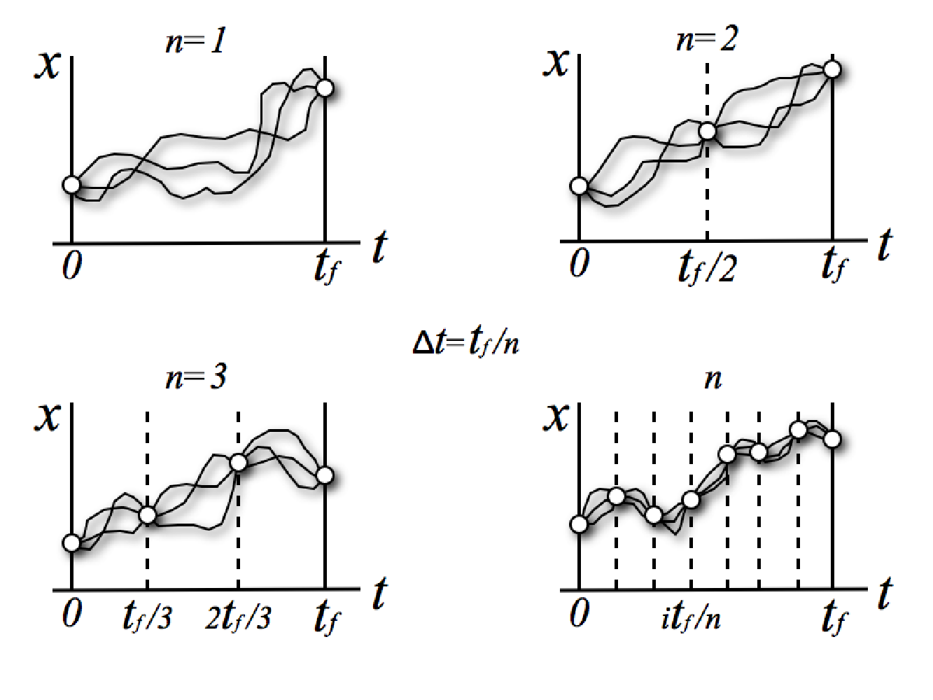
For simplicity we will consider that the coarse graining is into equal divisions of the total time duration . Therefore, in this -slicing procedure, the full trajectory of the particle is not measured but only its position after time intervals of duration . See figure 1. The probability for a discretized path can be easily evaluated since the process is Markovian and Gaussian. Let us denote by the conditional probability for jumping from a point at time to a point at time , and let be the initial equilibrium distribution. The probability of the -sliced discretized path is given by
| (13) | |||||
An analogous expression is valid for the backward path and probability, with superscript “tilde” again referring to time reversed excursion (trajectory and process). The central quantity we wish to evaluate is the following coarse-grained relative entropy ;
| (14) | |||||
Note that we have multiplied by (having absorbed in its units) since we want to compare the above expression with the dissipated work. The brackets refer to the average performed with the forward distribution, which weights every trajectory’s contribution.
The next step is to find the general expression for and . Since the Langevin equation that describes the dynamics is linear, the conditional probabilities are Gaussian distributions:
| (15) |
and
| (16) |
From equation (11) (applied for final and initial times and , respectively, and with the appropriate initial condition) the conditional averages are found to be
| (17) | |||||
| (18) |
where
| (19) |
Similarly, one can multiply the Langevin equation by the position and then take averages. This leads to the following equation for the variance :
| (20) |
which yields (conditional variances starting at zero value)
| (21) |
for both (forward and backward) cases.
In order to obtain , we insert the above conditional probability distributions in Eq. (14). The final result can most revealingly be written in terms of the duration of the experiment and the final position of the minimum of the trap . After some cumbersome calculations, one finally gets
| (22) |
First note that in the limit one finds (cf. Eq. (12))
| (23) |
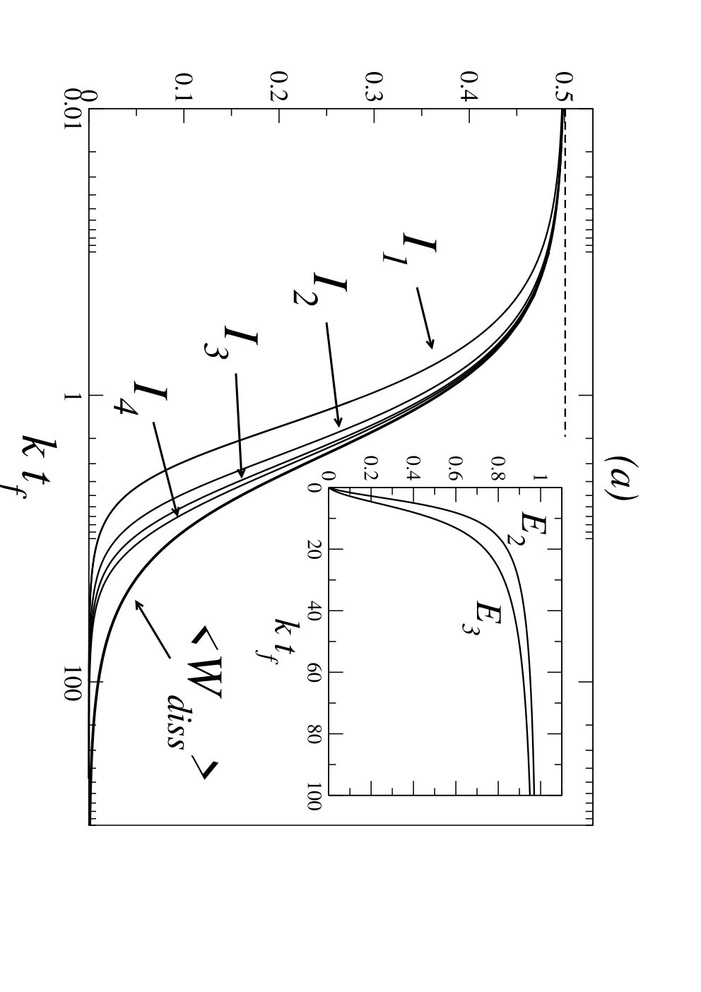
Hence the exact dissipation is, as anticipated, recovered in the limit of the continuous path description. We now turn to the following question. How is the convergence of to ? First, one can verify that, for any value of the system’s parameters, is always a lower bound for the total dissipation (cf. Eq. (5)):
| (24) |
Next, as is apparent from the explicit result (22) and scaling , the convergence of to depends only on the ratio of the time of the experiment over the relaxation time in the harmonic potential. In figure 2.(a) we plot up to , as a function of . The convergence is surprisingly good. For example, for , the error in (single intermediate measurement point, plus the initial and the final points, which are always measured) is only a few percent.
In the limit (or ), that is, for a very slow translation of the potential, one recovers the quasi-static result of zero dissipated work. Note however that the relative rate of convergence becomes quite bad in this limit (cf. inset in figure 2.(a)). On the other hand, the fit is perfect in the limit of the irreversible quench, in which the potential is instantaneously switched to its new position. This corresponds to the limit (or ). One finds
| (25) |
since the dissipated work is exactly equal to the average work done in instantaneously placing the particle in the shifted potential.
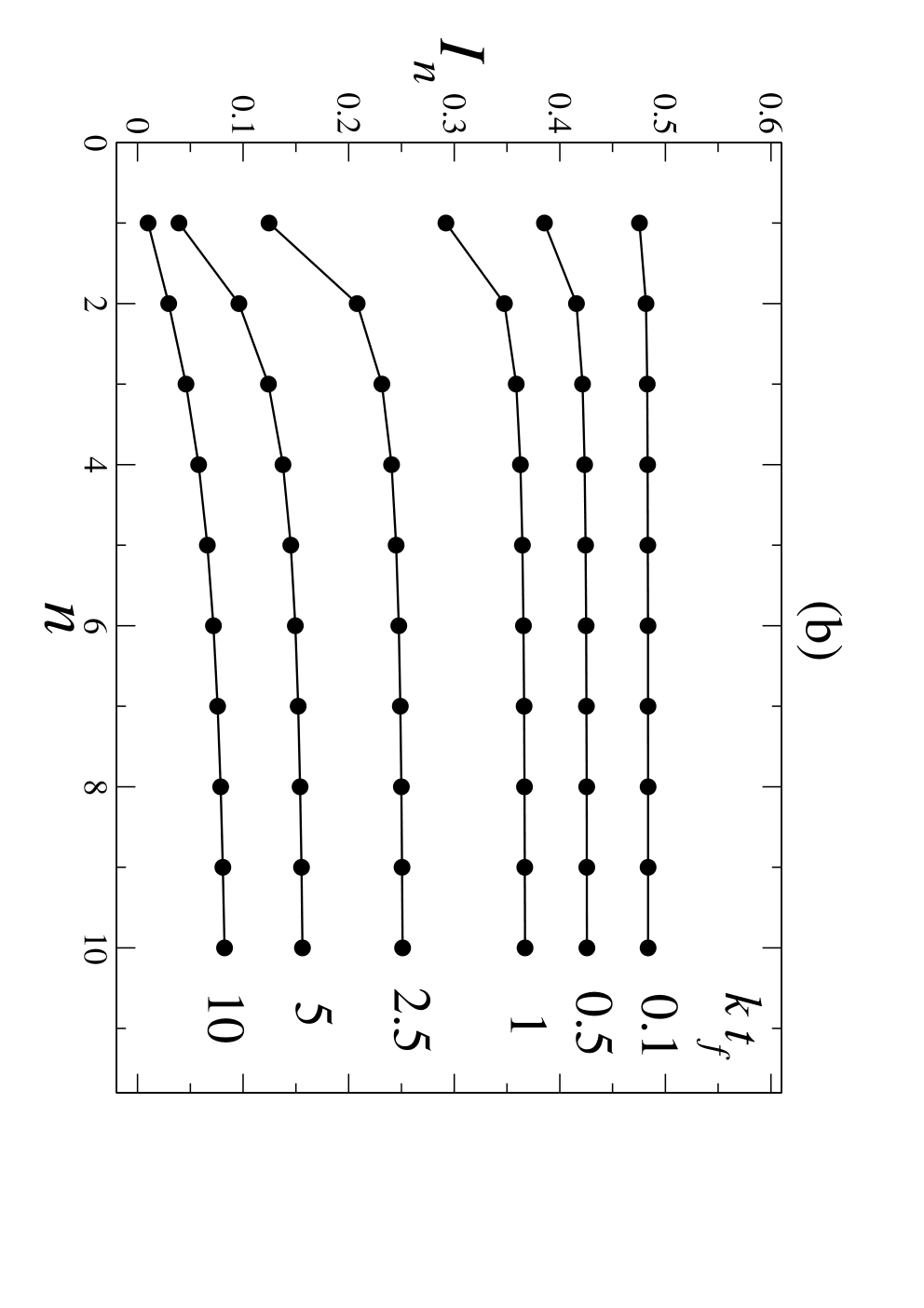
In Fig. 2.(b) we plot , for different values of , as a function of the number of measured points. Note that the biggest jumps in occur from to , after which the bound quickly saturates and slowly approaches the total mean dissipated work. The dominant term in the convergence of to is easily obtained from Eq. (22):
| (26) |
We expect that this type of convergence, , is valid for a continuous Markov process. There is a plausibility argument for this asymptotic behavior. The chain rule of the relative entropy, Eq. (3), implies
| (27) |
where stands for the “piece” of the trajectory with . Under the conditions , each of these pieces looks similar to the trajectories depicted in Fig. 1 and becomes a pinned diffusion process, which can be written as [42, 43]:
| (28) | |||||
where is a process satisfying the same dynamics as but with no restrictions. Averaging the above equation and assuming that is an analytical function of , one has:
| (29) |
Therefore, the averages of in the forward and backward processes can only differ by terms of order .
On the other hand, the relative entropy between two Gaussian distributions with the same dispersion and averages and is given by:
| (30) |
Let us assume that can be approximated by a Gaussian process with dispersion of order . If the external parameter does not affect the dispersion, the dominant term in the relative entropies in Eq. (27) will be given by the difference between averages, i.e., by Eq. (30):
| (31) |
If this is the case, then the asymptotic approach to the exact work is the same as in our example:
| (32) |
III.2 Underdamped Brownian particle in a suddenly quenched trap
In the previous example, we discussed the effect of coarse graining in time for the measurement of the single relevant variable at hand, namely the position of the overdamped Brownian particle. Now we address the additional question about the role of specific variables (or degrees of freedom) in revealing the dissipation. For the illustration of this point we naturally turn to underdamped Brownian particles, where both position and momentum of the particle are relevant. Instead of considering a moving harmonic potential with fixed strength, we study another experimentally significant scenario: a non-moving harmonic potential undergoing an instantaneous quench in its stiffness, say at the initial time from a frequency to the frequency . See the scheme in figure 3.
The average work dissipated in the instantaneous quench can be evaluated as follows. The potential energy of the particle when at a position , is given by , where is the harmonic frequency, with and before and after the quench, respectively. The probability distribution of the position at the moment of the quench is given by (as before, Boltzmann’s constant is absorbed in the temperature for simplicity of notation). Here , the normalization constant, is the familiar partition function. Averaging with respect to this distribution (notation ), we conclude that the average work associated to the quench is given by . The corresponding change in free energy is found to be . Therefore, the total dissipation in the irreversible instantaneous quench reads
| (33) |
Note that the total dissipated work is always positive due to the irreversible nature of the process.

As available statistical information we consider the probability distribution for position and momentum at a any single instant of time after the quench (see Fig. 3). As we have already shown in the first example, statistical information at just one particular time must provide a lower bound for the dissipated work corresponding to such quench:
| (34) |
Below we will elucidate the effect of such coarse-graining implied in the punctual measurement in time (at time after the quench) plus the effect of a reduction in the number of variables, this is, measuring only , only or both. We anticipate that this will lead to inequalities such as
| (35) | |||||
| (36) |
To explicitly obtain the bounds from the coarse-grained relative entropies appearing in equations (34), (35) and (36), we need to evaluate the probability distributions in forward and backward scenario. The derivation for the backward scenario is very simple; the system starts at canonical equilibrium with frequency and the quench is performed at the end of the experiment ( in forward time, which is the final time in the reverse experiment). The particle is then at canonical equilibrium with respect to the frequency throughout the process:
| (37) |
Note that the above distribution is even in , namely , and Gaussian with the following moments:
| (38) |
One the other hand, in the forward scenario, the initial condition is canonical with respect to the initial frequency , . At the frequency is suddenly changed to and then kept constant along the whole process and, therefore, the evolution of the system in the forward process consists of a relaxation to the new equilibrium state, . Then we are free to decide what we call the final time of the experiment and hence the choice of the measurement time after the quench is also completely free. We write the familiar equations of motion for such underdamped Brownian particle for ,
| (39) |
where is the friction coefficient, and is Gaussian white noise with strength determined by the fluctuation dissipation theorem, . The initial condition is stipulated by the fact that prior to the quench at , the system is at equilibrium in a harmonic potential with strength , i.e. it is bi-Gaussian with (cf. Eq. (38))
| (40) |
Since the Langevin equation is linear, the resulting time dependent probability distribution remains a Gaussian. Therefore, it is sufficient to evaluate the ensuing time evolution of first- and second-order moments. Since there is no shift in the center position of the harmonic potential, the average position and momentum stay equal to zero: . The second order moments obey the following evolution equations which are easily obtained from the evolution equations (39):
| (41) |
which have to be solved with the above mentioned initial conditions. One finds:
| (42) |
where
| (43) | |||
| (44) |
Note the switch from a monotonously decay ( real) to an oscillatory one ( imaginary) of the above solutions for the moments as crosses the value from below.
We are now in position to evaluate the relative entropy between and , which in this case can be considered as a distance between the relaxing time dependent distribution and its final equilibrium state , only reached for . Since both densities are Gaussian (and the backward distribution is even in ), the following result is obtained:
| (45) | |||||
where and are the covariance matrices of the forward and backward distributions, respectively
| (46) |
The above result can be further simplified to
| (47) |
From now on, subindices in refer to the variables contained in the probability distributions with which the relative entropy is evaluated. So when momentum is integrated out from the probability distribution, the relative entropy at time of the position distributions, , yields
| (48) |
and its momentum analog, , is
| (49) |
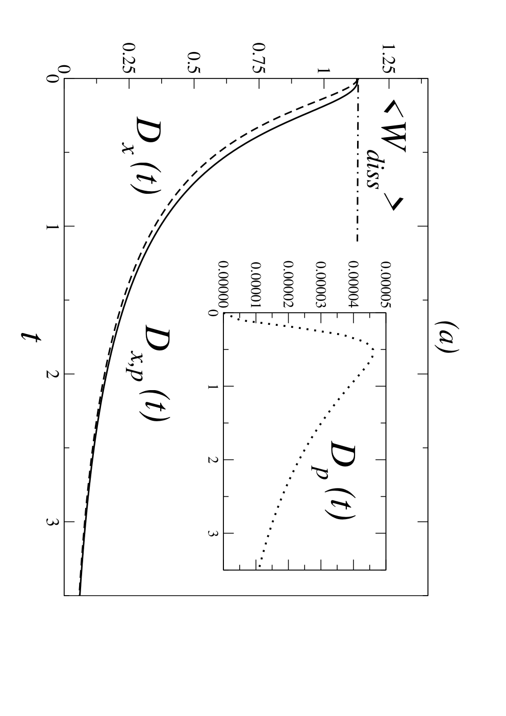
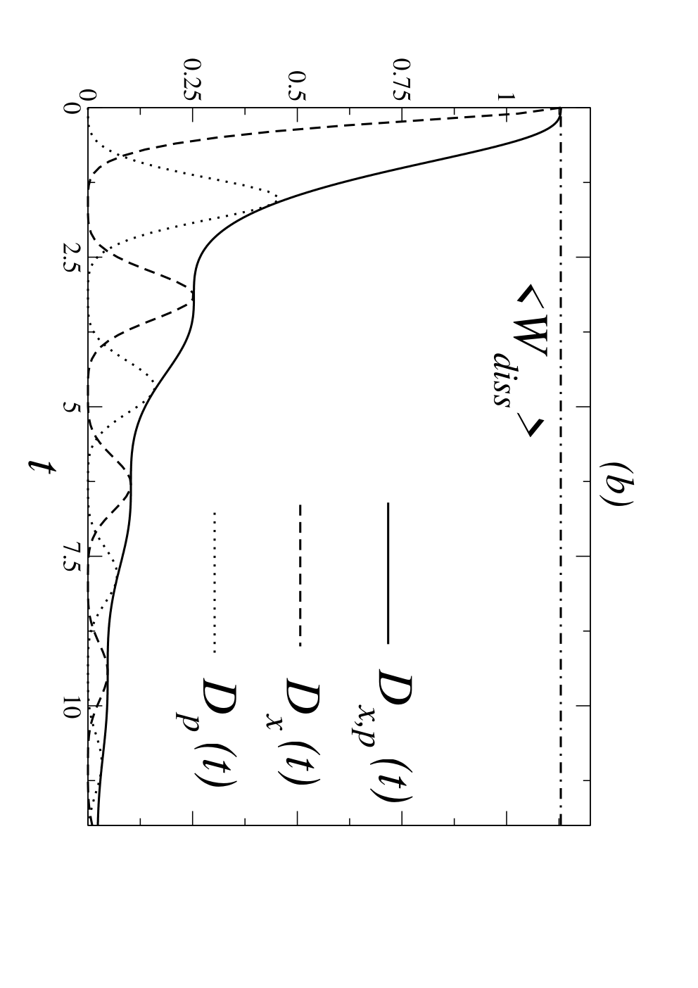
We insert in (47), (48) and (49) the expressions of the second moments calculated previously. With these explicit results (depicted in figure 4), we can discuss how well various relative entropies capture the information on the dissipation. First we note that at the moment of the quench (), the statistics of the position variable can account for the total work dissipated, , while no information is available from the momentum variable, . The reason is that the position at the time of quench is enough to evaluate the work [26].
Secondly, it is known that the relative entropy between the probability distribution of a Markov process and its corresponding stationary state is a strictly decreasing function of time [31]. Hence, must be so, as one can check from our calculations plotted in figure 4. On the other hand, when only one of the variables is taken into account, the relative entropies can exhibit a richer phenomenology. The behavior is rather different in the weakly damped regime than in the strongly damped one. In the strongly damped case () the relative entropies and just decay monotonically with time, see figure 4.(a). However, we obtain a non-monotonous behavior in the relative entropy of the momentum distribution, which is explained as follows. The equilibrium distribution of the momentum does not depend on the frequency of the oscillator. Therefore, at the quench time, the forward and backward momentum distributions are identical. However, once the potential is quenched, the momentum distribution will depart from equilibrium, due to transfers from potential to kinetic energy, to relax back to the same distribution at a later time. As a consequence increases from , reaches a maximum and decays back to zero for long time, as can be seen in the inset of figure 4.(a). The maximum is however very low, since damping is strong.
We can see a more pronounced and interesting effect in the underdamped case (). The main results are represented in figure 4.(b). Note the oscillatory exchange of information on dissipation between the position and velocity variables and the decay of the total information contained in . The behavior of and is induced by oscillations in the potential and kinetic energy of the particle. The relative entropy of the distributions can be written as (cfr. Eq. (48)):
| (50) |
where is the ratio between the potential energy at time and the equilibrium potential energy (at frequency ). A similar expression can be obtained for from Eq. (49). Therefore, the relative entropy of and can be considered as a measure of the departure of the potential and kinetic energy, respectively, from their equilibrium values. These energies turn to oscillate at frequency , twice the characteristic frequency of the damped oscillator.
The behavior of observed in Figure 4.(b) can be better understood by rewriting the relative entropy in (47) as follows:
| (51) |
where the correlation coefficient is given by
| (52) |
Since , we first note that the last term in the r.h.s of equation (51) is always positive, hence:
| (53) |
Therefore, in the present case, the sum of information on the dissipation gathered separately from position and momentum is smaller than that from both variables taken together. The equality sign in (53) is realized if , this is, when . From the oscillating analogue of the expression for in (42), one easily verifies that this occurs at specific times , where . Since the variables are Gaussian, the condition of zero correlation is tantamount to the independency of position and momentum.
Another interesting feature observed in figure 4 is that one of the variables, either or , loses all information on dissipation at another set of specific times. From equations (48) and (49) one finds that this occurs if or respectively. This is in agreement with the more general observation that the relative entropy of a specific degree of freedom is zero when, at a given time, the detailed balance condition holds, namely, when at that time the forward and backward distributions are equal.
On the whole, an intricate transfer of information on dissipation is taking place between position and momentum of the underdamped Brownian particle. At the same time, such information on the total mean dissipated work is irreversibly lost by the punctual (one-time) relative entropy of and and transfered to the heat bath variables as time goes by.
III.3 Flow of information between coupled oscillators.

To complete the picture, we next consider the case of a harmonically bound underdamped Brownian particle that is indirectly in contact (via a second Brownian particle) to a heat bath. The idea is that, by monitoring this second particle, we are including some information on the heat bath, of which it is supposed to be part. The Langevin equations of motion that describe the system read:
| (54) | |||||
| (55) |
where . As in the previous case, we consider the quench experiment: oscillator is initially prepared in equilibrium with . At we perform an instantaneous quench switching so that for . Oscillator is kept throughout at the same frequency , linearly coupled to oscillator with a strength and immersed in the heat bath, which is modeled by means of a fluctuating force and a friction term proportional to . See figure 5.
The time dependent probability distribution that characterizes the evolution of the whole system is a Gaussian, whose first moments are simply
| (56) |
Thus we need to evaluate the second moments which, having defined and , obey the following set of evolution equations:
| (57) |
The system can be solved explicitly using the appropriate initial conditions corresponding to the equilibrium ensemble. However, the analytic expressions are extremely lengthy. In what follows, we will illustrate the obtained behavior via figures.
Since the joint distribution is Gaussian (and the backwards density even in ), the relative entropy involving all four variables and can be compactly expressed in terms of the covariance matrices and :
| (58) |
The latter are the following four-by-four symmetric matrices
| (59) |
and for the covariance matrix corresponding to the backwards excursion we explicitly find
| (60) |
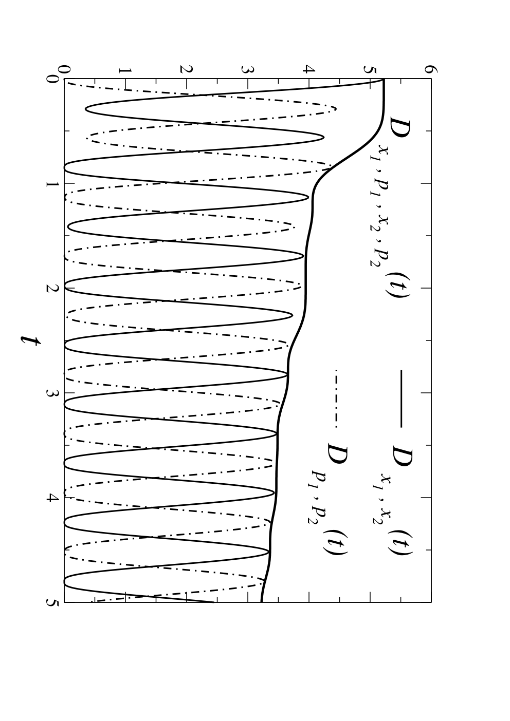
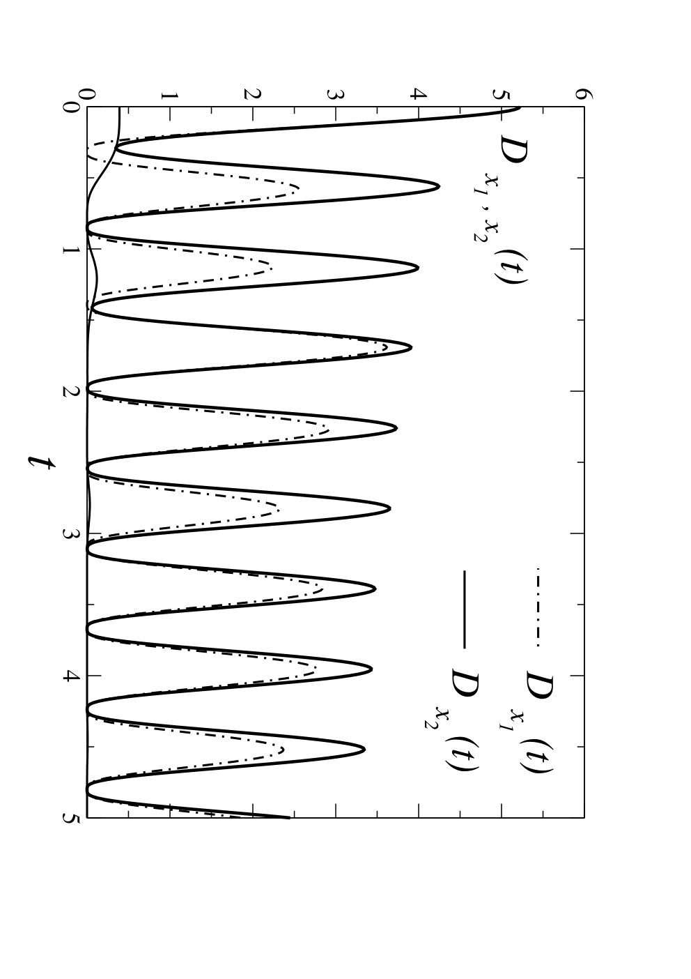
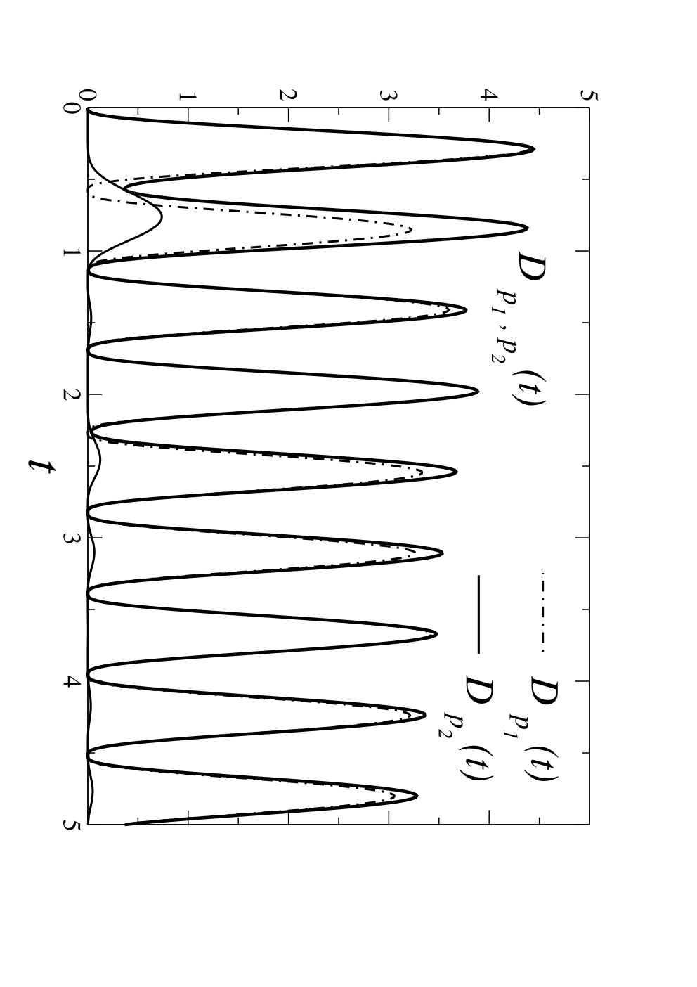
From the above results, we can derive the relative entropy of all available degrees of freedom of the system (both positions and , and momenta and ), along the whole time track with a single time measurement. Similarly to the underdamped oscillator case of the previous section, one can explore the behavior of the relative entropies of all possible combinations of the degrees of freedom. Some of them are plotted in figure 6. All the features of the model in the previous section are found here too: the relative entropy of the whole system, , decays monotonically in time and it is an upper bound with respect to any other relative entropy accounting for less degrees of freedom. The relative entropy of subsystem , , is oscillating in an intrincate manner below the former, together with and , which transfer information periodically and are modulated by . Again, only when performed at the moment of the quench does the measurement concerning the position contain full information.
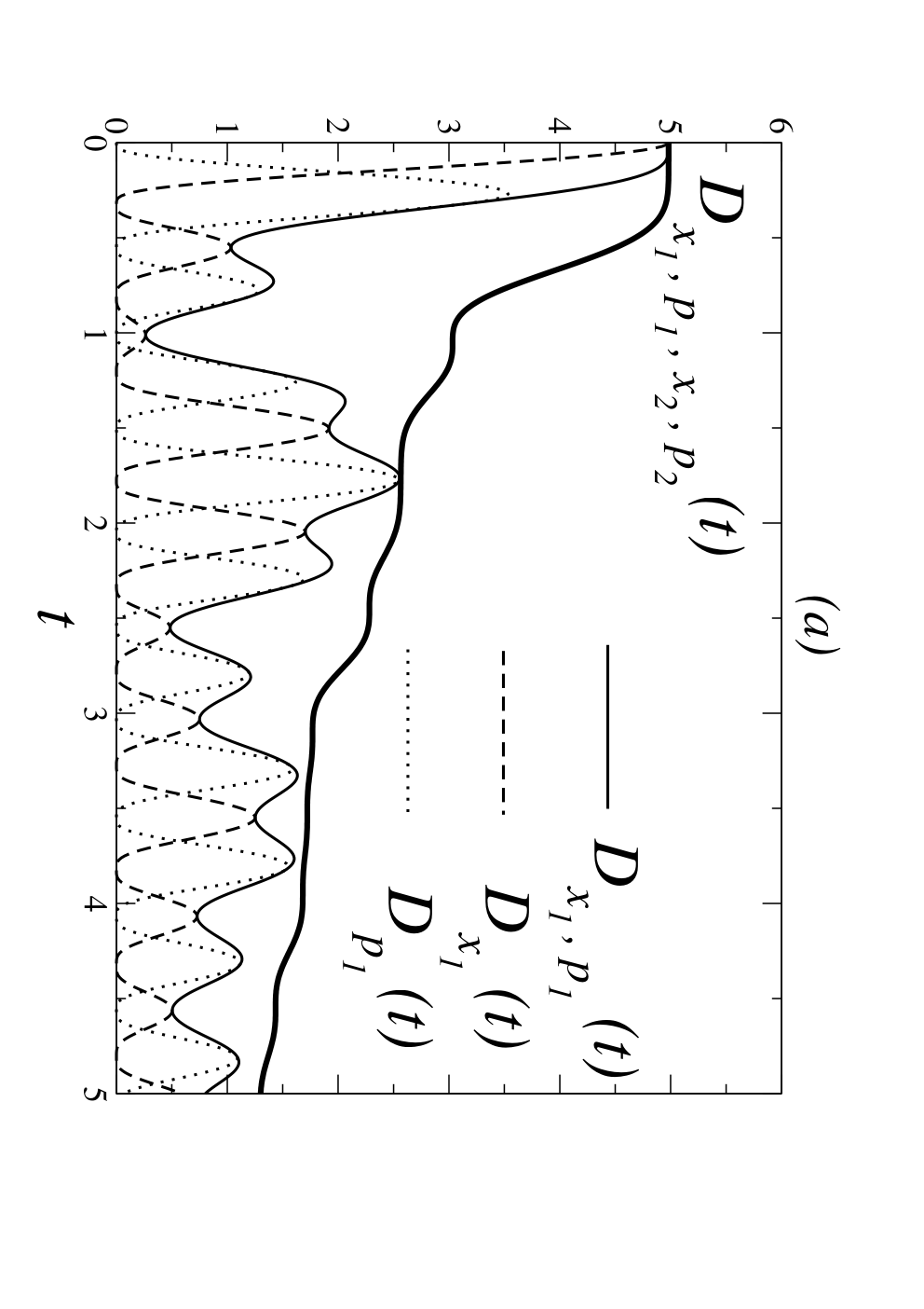
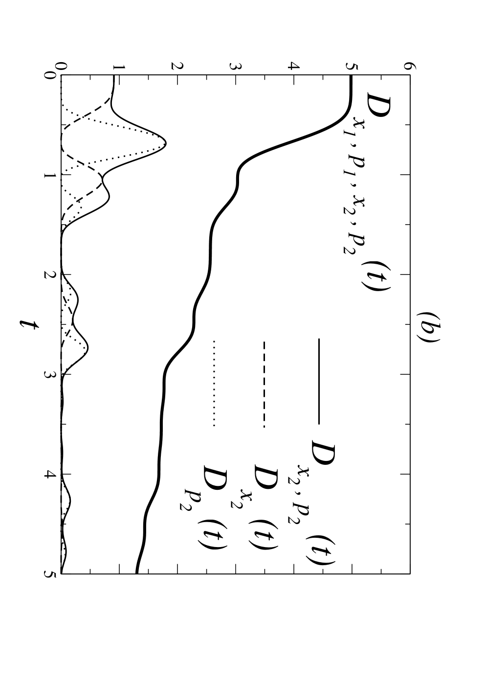
The novelty in this case is that oscillator is not directly in contact with the heat bath, but indirectly through oscillator . This allows for a more detailed study of how the information on dissipation contained in the first subsystem leaks out irreversibly. First it has to flow to the second subsystem and then it is dumped into the heat bath variables, where it is forever lost. Comparing figure 6.(a) with 6.(b) we see that the relative entropies of oscillator are significantly smaller than those of oscillator . The former receives information on the dissipated work at the quench only through its coupling to and, while it bounces back some of this information to , its relative entropy decays much faster because it is directly connected to the heat bath.
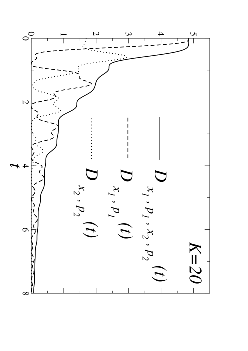
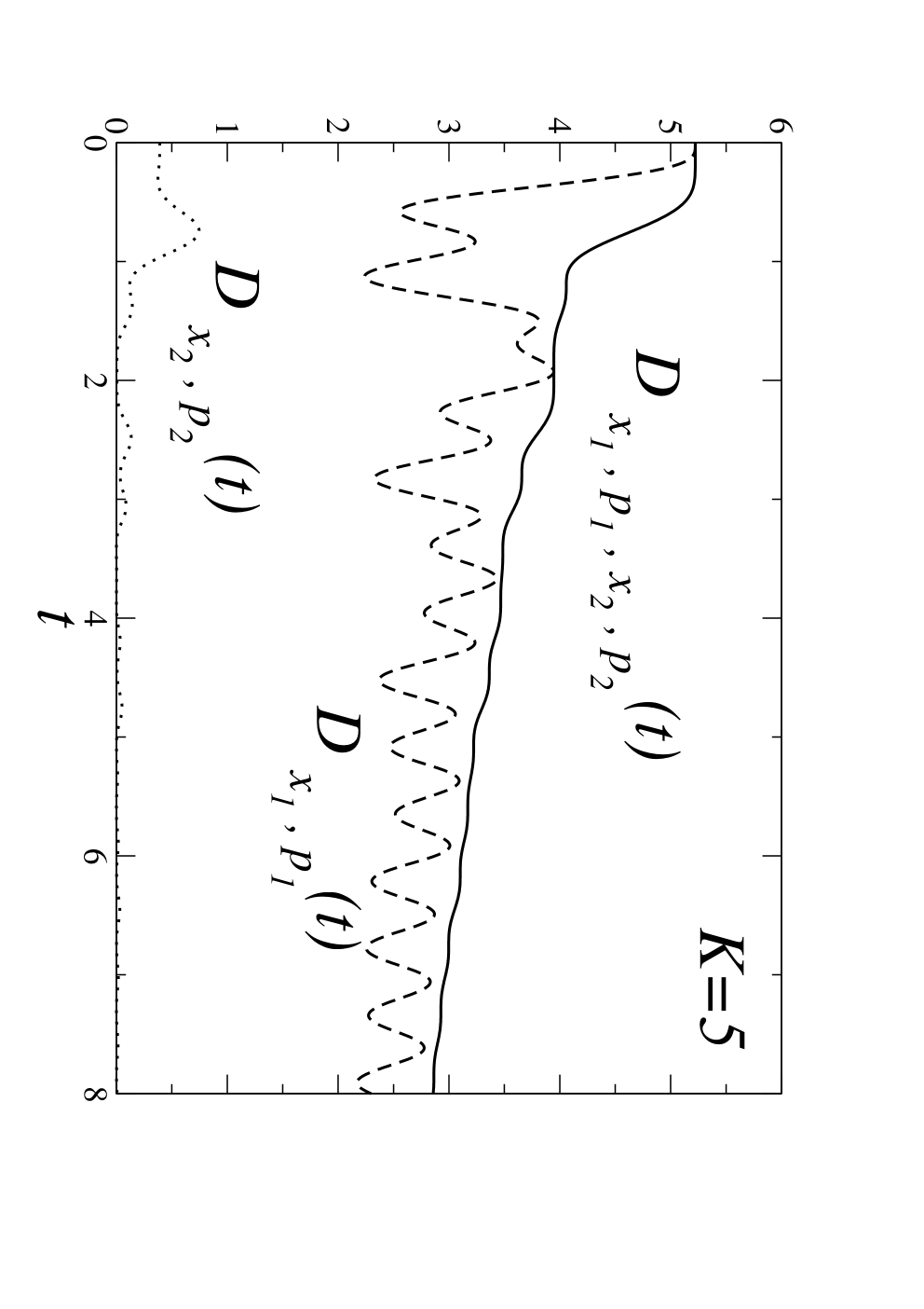
The plateau for the relative entropy appearing at short times in figure 6 shows that most of the effect of the dissipative process (the irreversible quench) still resides inside the system formed by the two particles. In fact, oscillator keeps much of this information while slowly transferring it to oscillator . This depends on the coupling constant hat connects both oscillators. This dependence is illustrated in figure 7. For the general decay is fast since both subsystems are well coupled and information on the quench can quickly flow to the heat bath. However, for such flow is reduced and the relative entropy of oscillator is almost zero but yet there is a considerable difference between and . Therefore, while oscillator is “close to equilibrium”, its correlation with oscillator still carries relevant information on the irreversible quench. This conclusion is valid both for positions and momenta, separately, as seen in Fig. 8 for . As in the case of a single oscillator, information flows from positions to momenta, but is mainly kept by the quenched oscillator or by correlations with oscillator 2, which rapidly reaches equilibrium.
IV Conclusions
Dissipation is related to our ability to distinguish the arrow of time. As was anticipated in earlier work in the literature, we find that dissipation is proportional to the relative entropy between the probability distributions of forward and backward excursions, respectively. We have exploited such expression in terms of relative entropy to give rise to lower bounds for the dissipation if only partial information on the trajectories is available.
Several scenarios have been discussed in order to illustrate how dissipation can be bounded from below on the basis of reduced information. First, when coarse-graining the continuous trajectory of the system into a reduced finite number of measurements, our analysis has shown that the resulting relative entropy provides reasonably accurate bounds for the dissipation, even with only a small number of intermediate measurement points. As a generalization of our findings in this specific example, we conjecture that the relative entropy obtained from measurements approaches the exact value of the dissipation as , for large. These results could be especially useful in real experiments where trajectories are recorded at finite sampling rates.
Second, we have analyzed the effect of considering a subset of variables instead of a detailed description of the system in a quench process. In this case, the time-arrow information, concentrated in the single position variable immediately after the quench, is subsequently transferred to the thermal bath and the other variables. Of special interest is the case of two oscillators, the first one undergoing a quench of its frequency and the second one in contact with a thermal bath. We recall that the relative entropy is constant when all the degrees of freedom of a Hamiltonian system are taken into account [25]. One could then expect that the information contained in the first oscillator would be transferred to the second one before getting lost in the thermal bath. However, our analysis calls into question this naive picture, as we have shown that the oscillator coupled to the thermal bath is the first to thermalize. The information on the dissipation is mainly kept by the first oscillator or by correlations between the two. The generalization of our analysis to long chains of oscillators will help to further elucidate how information is spread along many degrees of freedom.
We acknowledge financial help from the Ministerio de Educacion y Ciencia (Spain) under Grants FPU-AP-2004-0770 (A. G–M.) and MOSAICO (JMRP), and from the FWO Vlaanderen.
References
- [1] L. Onsager, Phys. Rev. 37, 405 (1931).
- [2] L. Onsager, Phys. Rev. 38, 2265 (1932).
- [3] I. Prigogine, Etude Thermodynamique des Phénomènes Irréversibles ( Desoer, Liège) 1947.
- [4] S. R. de Groot and P. Mazur, Non-Equilibrium Thermodynamics (Dover, New York) 1984.
- [5] D. J. Evans, E. G. D. Cohen, and G. P. Morriss, Phys. Rev. Lett. 71, 2401 (1993).
- [6] G. Gallavotti and E. G. D. Cohen, J. Stat. Phys. 80, 931 (1995).
- [7] J. Kurchan, J. Phys. A 31, 3719 (1998).
- [8] J. L. Lebowitz and H. Spohn, J. Stat. Phys. 95, 333 (1999).
- [9] C. Maes, J. Stat. Phys. 95, 367 (1999).
- [10] G. N. Bochkov and Yu. E. Kuzovlev, Zh. Eksp. Teor. Fiz. 72, 238 (1977).
- [11] G. N. Bochkov and Yu. E. Kuzovlev, Sov. Phys. JETP 45, 125 (1977).
- [12] G. N. Bochkov and Yu. E. Kuzovlev, Physica A 106, 443 (1981).
- [13] G. N. Bochkov and Yu. E. Kuzovlev, Physica A 106, 480 (1981).
- [14] C. Jarzynski, Phys. Rev. Lett. 78, 2690 (1997).
- [15] C. Jarzynski, Phys. Rev. E 56, 5018 (1997).
- [16] G. E. Crooks, Phys. Rev. E 60, 2721 (1999).
- [17] T. Hatano and S. I. Sasa, Phys. Rev. Lett. 86, 3463 (2001).
- [18] B. Cleuren, C. Van den Broeck and R. Kawai, Phys. Rev. Lett. 96, 050601 (2006).
- [19] G. E. Crooks, J. Stat. Phys. 90, 1481 (1998).
- [20] C. Maes and K. Netocÿny, J. Stat. Phys. 110, 269 (2003).
- [21] U. Seifert, Phys. Rev. Lett. 95, 040602 (2005).
- [22] P. Gaspard, J. Stat. Phys. 117, 599 (2004).
- [23] Jiu-Li Luo, C. Van den Broeck and G. Nicolis, Z. Phys. B 56, 165 (1984).
- [24] J. Schnakenberg, Rev. Mod. Phys. 48, 571 (1976).
- [25] R. Kawai, J. M. R. Parrondo and C. Van den Broeck, Phys. Rev. Lett. 98, 080602 (2007).
- [26] A. Gomez-Marin, J. M. R. Parrondo and C. Van den Broeck, EPL, 82 50002 (2008).
- [27] C. Jarzynski, Phys. Rev. E 73, 046105 (2006).
- [28] S. Rahav and C. Jarzynski, J. Stat. Mech.: Theory Exp. (2007) P09012.
- [29] R. A. Blythe, Phys. Rev. Lett. 100, 010601 (2008).
- [30] D. Andrieux, P. Gaspard, S. Ciliberto, N. Garnier, S. Joubaud and A. Petrosyan, Phys. Rev. Lett. 98, 150601 (2007).
- [31] T. M. Cover and J. A. Thomas, Elements of Information Theory, 2nd ed (Wiley, Hoboken, NJ) 2006.
- [32] E. H. Trepagnier, C.Jarzynski, F. Ritort, G. E. Crooks, C. Bustamante and J. Liphardt, Proc. Nat. Acad. Sci. 101 15038 (2005).
- [33] K. Sekimoto, J. Phys. Soc. Jpn. 66, 1234 (1997).
- [34] K. Sekimoto, Prog. Theor. Phys. Suppl. 130, 17 (1998).
- [35] J. Farago, J. Stat. Phys. 107, 781 (2002); Physica A 331, 69 (2004).
- [36] R. van Zon and E. G. D. Cohen, Phys. Rev. Lett. 91, 110601 (2003).
- [37] V. Blickle, T. Speck, L. Helden, U. Seifert and C. Bechinger, Phys. Rev. Lett. 96, 070603 (2006).
- [38] A. Gomez-Marin and J. M. Sancho, Phys. Rev. E 73, 045101(R) (2006).
- [39] P. Visco, J. Stat. Mech.: Theory Exp. P06006 (2006).
- [40] M. Baiesi, T. Jacobs, C. Maes and N. S. Skantzos, Phys. Rev. E 74, 021111 (2006).
- [41] F. Douarche, S. Joubaud, N.B. Garnier, A. Petrosyan and S. Ciliberto, Phys. Rev. Lett. 97, 140603 (2006).
- [42] T. Misawa, J. Math. Phys. 34, 775 (1993).
- [43] T. Misawa and H. Itakura, Phys. Rev. E 51, 254 (1995).