Wigner islands with electrons over helium
Abstract
We present here the first experimental study of Wigner islands formed by electrons floating over helium. Electrons are trapped electrostatically in a mesoscopic structure covered with a helium film, behaving as a quantum dot. By removing electrons one by one, we are able to find the addition spectrum, i.e. the energy required to add (or extract) one electron from the trap with occupation number . Experimental addition spectra are compared with Monte Carlo simulations for the actual trap geometry, confirming the ordered state of electrons over helium in the island.
pacs
67 40I Introduction
Electrons collect on a two-dimensional sheet when they are spread over the surface of a liquid helium film. This is due to the attractive charge which appears by polarisation of the helium. Due to the weakness of the image charge, electrons sit in the vacuum far away from the surface and move freely at a fixed distance over the film. As such, they constitute a very clean and predictable system.
When temperature is reduced, kinetic energy decreases relative to Coulomb energy; correlations begin to dominate the electronic structure. Wigner predicted in 1934 that a phase transition would take place in the infinitely extended system, leading to the formation of a two-dimensional (2D) electron lattice.[1] Wigner crystallisation into a triangular lattice of electrons over helium has been observed first by Grimes and Adams.[2, 3] This phase transition takes place below a transition temperature that is a function of electronic density. For the infinite system in the classical limit,[4] in which particles can be treated individually and which is mostly appropriate for electrons over helium, the transition occurs when the ratio of the average Coulomb interaction energy to the thermal energy becomes greater than 137. In the quantum case, eventually reached at low enough temperatures, the Wigner solid is predicted to form when the Brueckner parameter , the interelectron distance normalised by the Bohr radius, , becomes smaller than 37. Recently, somewhat more complex phases and ordering transitions have been predicted around that threshold.[5, 6]
An assembly of rectilinear vortices provides another example of Wigner lattice formation.[7, 8] Abrikosov’s triangular lattice for vortices induced by magnetic fields in type II superconductors [9] was first observed indirectly by neutron diffraction [10] and later visualised directly by electron microscopy imaging by Bitter decoration of the trapped flux lines with ferromagnetic microparticles.[11]
Also, electrons in semiconductor heterostructures localised by an applied magnetic field undergo a magnetically induced Wigner transition. [12] They form a well-studied and well-understood system, the quantum dot, which has been the object of extensive research for the past two decades.[13]
I.1 Confined electron structures
When confining 2D-electrons to a restricted planar area, the breaking of translation invariance brings in important changes with respect to the infinite geometry case, in particular because thermodynamic phase transitions are suppressed by fluctuations. This problem of 2D ordering in restricted geometries has been extensively studied theoretically, mostly for parabolic traps with Coulomb interaction between the electrons, first in the limit where electrons behave as classical particles,[8, 14, 15, 16], next in the computationally more demanding quantum case.[17, 18, 19, 20]
Finite-size effects become prevalent for . Such is the case in the work described below. New features appear that depend on the competition between the triangular lattice, which takes over for sufficiently large systems, and the shape and strength of the confining potential, which tends to suppress it. For hard confining walls and a flat trap bottom, it is predicted that the ordering is mostly affected close to the boundaries, electrons in the interior of the 2D island retaining the triangular lattice structure. For traps with a parabolic confining potential, the particles arrange themselves in circular shells with widths small compared to the radius of the shell. Thus, even with very few electrons, ordered structures can appear, the Wigner molecules.
The direct observation of such structures in restricted geometry has been achieved only for systems of macroscopic charged particles,[21] and for vortices in superconductors[22] and superfluid helium.[23, 24]
For electrons over helium, finite islands of electrons can now be realised [25] so that well-controlled experiments can be conducted on this very clean system, which we report here. Direct (visual) observation of the electronic structure cannot be performed in the present experiments: the geometric arrangement of the electrons in the island must be deduced from properties such as their escape energy from the island.
I.2 Wigner molecules
Contrarily to solid-state quantum dots, for which interactions between electrons decrease exponentially due to the screening from surrounding electrodes, electrons over helium are located far from conducting bodies; the Coulomb interaction is mostly unscreened and gives rise to strong, long-range, interparticle correlations. Also, there are no nearby impurity, no effective mass correction; image charges are well-defined. These features concur to make Wigner islands of electrons over helium an ideal model for the study of strongly correlated few-body fermionic systems.
The electron states and energies depend markedly on the trap geometry and on the details of the interparticle interaction, which in turn depends on the number of electrons in the trap and their arrangement. For traps with steep walls and flat bottoms, the electrons tend to form a triangular lattice in the island interior and adjust to the walls at the trap periphery with a disorganised layer. For circular parabolic traps, electrons order first on concentric shells following a Hund-type law.[14] These structures are referred to as Wigner molecules.
When fluctuations, either thermal or quantum, are further reduced by lowering the temperature or by adjusting the electron areal density, the angular positions of the various shells become locked: orientational order sets in amongst the previously radially ordered electrons. Some particularly stable configurations are found that correspond to “magic numbers” of electrons with high ordering temperatures while other trap occupation numbers lead to less stable structures and lower ordering temperatures.

I.3 “Phase” diagram
The various ordering processes taking place in 2D-clusters of electrons - the Wigner islands - and the formation of radially correlated structures - the Wigner molecules - have been the subject of a large number of theoretical studies. Our interest here lies in systems with a small number of electrons, , confined in relatively large traps so that the electronic density is low.
The behaviour of electrons freely suspended in vacuum over liquid helium and confined laterally in a circular parabolic trap by a potential , being the bare electron mass and the harmonic trap frequency, is described by the following Hamiltonian
| (1) |
The terms in curly brackets describe noninteracting electrons in the trap. The characteristic length associated with these two terms can be viewed as the spatial extent of the electron motion. The Coulomb interaction, the last term in Eq.(1), eventually localises and orders the electrons within the trap to distances of the order of such that . Following Filinov et al.[18], we can therefore take the quantity , which represents the fraction of the trap area actually occupied by the electrons, a dimensionless measure of the electronic areal density.
The configuration and energies of Wigner islands with electrons are described by Eq.(1), the eigenstates of which however can be found analytically only for .[26] Various approximation schemes have to be used for higher occupation number.[27, 28, 29] Larger electron islands require the recourse to numerical simulations (see, for a review, Reimann and Manninen[20]). Interactions with the environment - heat bath and measuring equipment - are not included in Eq.(1). In the simulations of Filinov et al.[18] the temperature comes in as an input in the Monte-Carlo simulations.
A generalised “phase” diagram for the various ordering processes - radial and orientational - taking place in Wigner islands with few electrons has been constructed numerically by Filinov et al.[18] whose findings are sketched in Fig.1. These authors characterise the onset of order by looking at the correlations between electrons both radially and angular-wise. In the ordered state, they find that , introduced above on dimensional grounds, is quite close to the mean interparticle distance defined by the first maximum of the pair distribution function. When coming from the dense, hot (large or/and ) regions of the diagram, where the 2D electron cluster is in a disordered (liquid or gas-like) state and moving to more dilute, cooler region, boundary lines are found first to the radially ordered state (RM), and, moving further in, to complete ordering where the orientation of the various shells become frozen with respect to one another (OM).
I.4 Electronic configurations
As seen in Fig.1, Wigner ordering takes place at low densities and low reduced temperatures along boundaries that differ markedly for various occupation numbers . Some clusters are more stable than others. Specifically, clusters with 11 and 20 in Fig.1 melt radially at higher , but orientationally at much lower values of .[18] The orientationally more stable clusters are called magic clusters, =10, 12, 16, 19 in Ref.[18], and possess a fully frozen structure that is closest to the Wigner triangular lattice so that the shells cannot rotate on one another. Those that can, =11, 20, are far less stable orientationally, but a little more stable radially.
Somewhat surprisingly, these more radially stable configurations turn out to be even more stable than the homogeneous Wigner crystal itself, which melts in the classical limit for temperatures above that set by . For the full quantum case, the critical melting density for the homogeneous system is set by the value of the Brueckner parameter . The Brueckner parameter can be extended to finite systems by taking the definition of in an electron cluster given above, which yields . All boundary lines in Fig.1 lie below the melting curve for the quantum Wigner crystal.
It should be mentioned however that these boundaries do not correspond to sharp transitions between electronic structures with different types of order. The localisation process of the electrons into organised structures takes place gradually only, as stressed by Ghosal et al. [6] in particular.
Also, considerably lower critical values for , down to 4, corresponding to much higher critical densities, have been reported for clusters with few electrons.[17] However, these findings seem to be an artifact of the computational scheme and are not confirmed in subsequent work.[30, 31, 6] It thus does appear, as shown in Fig.1, that the critical density beyond which quantum fluctuations dominate, destroying the ordered phase of 2D confined structures remains of the same order of magnitude as for the open-geometry situation when the number of particles, , is large.
Detailed studies of the ordered configuration of these few-body clusters have been performed, mostly by numerical simulations, both for systems of vortices in rotating helium and superconducting disks,[7, 8, 32] and in quantum dots by a number of authors, notably Peeters et al.[14, 15, 33] in the classical limit, to whose work we compare our own simulations in Sec.IV below.
Visual observations of the ordering of small charged metallic spheres confined in circular trap on a plane have been performed by Saint-Jean et al. [21] Somewhat unexpectedly, their observations of the ground state configuration of clusters with up to 30 led to significant differences with the predictions for some of the structures simulated by more sophisticated Monte-Carlo (MC) and molecular dynamics (MD) techniques.[34, 14, 15, 35] They however agreed with the structures found in older work based on a spatial step-by-step minimisation of the free energy.[8] For instance, the cluster with is found to order in the ground state with an inner shell of 4 electrons[8] against 5 electrons in MC-MD calculations. In other words, an outer shell with is favoured by the Monte Carlo approach compared to one with in the spatial minimisation procedure. Likewise, for a cluster with , the observed structure has two shells, 5 electrons on the inner shell and 11 on the outer. The MC-MD structure would comprise three shells, one electron at the centre, 5 and 10 on the two other shells.
The MC approach has been reexamined by Kong et al. [36] in order to resolve this discrepancy. These authors paid careful attention to the metastable states and the saddle paths between them. They confirm the findings of earlier work with the same computational technique (see also Kong et al. [37]). Noting that the energy difference between the true ground state for and 16 - in their calculation - and the closest metastable state - observed as ground state by Saint-Jean et al. [21] is quite small, these authors suggest that either the experimental situation differs from the one described by the simulation, or the observed configuration gets consistently stuck in the metastable state. The precise cause for the discrepancy is not really uncovered yet although there are hints that electron structures are quite sensitive to the exact shape of the potential: a departure from a parabolic confinement potential going as with to one with is enough to alter the computed structures and restore agreement with experiment.[36, 38] We shall thus consider that MC calculations carried out with the actual confining potential do lead to results in agreement with experiments.

I.5 Addition spectra
Addition spectra are built from the energy required to add one extra electron in the trap. This energy equals the difference in chemical potentials between clusters with and electrons:
| (2) |
being the ground state energy of the cluster with electrons. Once this last quantity has been determined numerically, the values of the experimentally more accessible quantity are known. A study of the details of this spectrum thus gives a map of the -electron cluster ground state energies and provides clues about the occurrence of ordering in the Wigner island.
As it became appreciated that addition spectra provide experimentally accessible signatures of the onset for the formation of shells in Wigner molecules,[39] detailed theoretical predictions for various confinement potentials appeared in the literature (see the reviews by Kouvenhoven et al. [40] or Reimann and Manninen [20], and, for more recent work, notably Ghosal et al. [6] and Güçlü et al. [41]).
In the weakly-interacting case, when the last term of the right hand side of Eq.(1) gives a negligible contribution, the quantity remains small as shells simply fill in and . When adding one electron gets a new shell started, for , the addition energy shows spikes that reveal the shell structure of the 2D harmonic confinement potential.
As the confinement potential decreases with respect to the Coulomb interaction contribution, i.e, as the electron density diminishes, the Wigner triangular lattice structure eventually forces its imprint on the electron cluster. A new addition energy signature appears with peaks at .[41] The crossover occurs around : denser clusters are in a liquid-like state, thinner ones gradually develop a crystal-like state. As emphasised by Ghosal et al. [6] the transition is smooth; addition spectra are expected to change gradually from shell formations to full spatial ordering. The “phase” diagram in Fig.1 shows different thresholds for the onset of order as revealed by the study of pair correlations.[18] It however exhibits the same qualitative trend in the ordering sequence of the electron islands, which can be studied by measuring the addition spectra.
Our goal in the work reported here is a comparison between the addition spectra observed in the trap for electrons over helium used experimentally and the outcome of numerical simulations that we have performed using the known geometry of the trap. This trap is described in Sec.II, the experimental procedure in Sec.III, the obtained spectra in Sec.IV, and the numerical simulations in Sec.V.
II The electron trap
The trap used in the present work to confine electrons to a 2D island is simple compared to other traps used for charged particles, which are usually closed by radiofrequency fields. Here, the electron motion is restricted along a plane, on the one side, by the free surface of liquid helium that presents an energy barrier of eV to the electron, on the other side, by the image charge in the fluid bulk that provides electrostatic attraction.
At temperatures below 1 K the saturated vapour pressure of helium is very low: electrons float above the surface of helium in near absolute vacuum. Unlike solids, liquid helium contains no impurities. Its topological defects - the vortices - and its elementary excitations - the phonons, rotons and ripplons - are well known, allowing relatively simple calculations of interactions between the object in the trap and the environment.[42, 43, 44] A comprehensive review of the physics of electrons on liquid helium can be found in Ref.[45].
The free electron is attracted toward the helium surface by its image charge and is repelled by the 1 eV barrier for entering the liquid bulk; it forms what can be viewed as a one-dimensional hydrogen-like atom. The dielectric constant of helium is low () and the image charge , being the electron charge, is small. The characteristic lengthscale analogous to the Bohr radius is Å, being the bare electron mass, is much larger than the atomic scale. The electron in its ground state is floating at Å above the helium surface. An electric field can be applied externally to press the electron on the surface and tune both its height and energy.
If unconfined laterally, the electron moves freely over the surface of bulk helium. Its mobility is the highest of all condensed matter systems.[46] The transverse motion of the electron can be restricted by a system of electrodes located below the helium surface. The micro-fabricated device used in the present work is shown in Fig.2 and is described in full detail in Ref.[47].
The right panel of Fig.2 shows the trap where electrons form a Wigner island. It is a three dimensional structure micro-machined on a silicon wafer consisting of i) a system of electrodes designed to hold the electrons in a well-defined position over the liquid helium surface, ii) a single electron transistor (SET) on a pyramidal island at the centre of the trap used to detect the presence of electronic charges and, possibly, the excitation state of the cluster. The pyramidal shape was made with a 5-angle evaporation procedure based on the well-known shadow technique. All electrodes are made of niobium except the SET which is made of aluminium. More details are given in Ref.[48].
The trap and the reservoir, shown in the left panel of Fig.2, are 600 nm lower than the surrounding guard electrode. Both are filled with liquid helium. The long rectangular region acts as a reservoir for surface electrons storage. If all electrons in the trap happen to become lost, the trap can be replenished by tapping the reservoir. The guard electrode is made out of a thick (0.25 µm) layer of Nb deposited on an insulating layer of comparable thickness. This electrode is used to support, by surface tension, the helium film over the reservoir and the trap ring, so that the liquid depth is µm. The electrode itself and the rest of the sample are covered by a thin (200-400 Å) film of helium, held by Van der Waals attraction. The bottom of the reservoir is covered by two electrodes, made out of thin niobium. These separate electrodes control the potentials of the right and left halves of the reservoir. They are used to shuffle electrons from one side to the other. The resulting change in capacitance provides a mean of gauging the total mobile charge contained in the reservoir.
A gorge through the guard electrodes connects the reservoir to the trap. Usually, the guard electrode is biased to negative potential relative to the SET. A potential barrier thus forms at the gorge, separating the trap and the reservoir. As the right reservoir electrode protrudes inside the gorge, the potential on this electrode strongly affects the height of this barrier. Typical potential profiles formed by these electrodes are shown in Fig.3. All electrodes are capacitively coupled to the SET island and can be used as gates.
The geometric radius of the trap is 3 µm, but its effective radius is significantly smaller and depends on the configuration of the electrostatic potentials on the various neighbouring electrodes. The actual potential well is neither parabolic nor axisymmetric. Both shape and depth change with the voltage applied to the electrodes. It becomes shallower when the lability point, at which the confinement completely disappears, is approached. To set numbers, a trap frequency of of 40 Ghz represents a low estimate when the trap holds few electrons only. The extension of the ground state wavefunction of non-interacting electrons is then nm. The mean distance between interacting electrons fixed by the Coulomb energy and the parabolic confining energy is 200 nm, the average density parameter , 0.016, the Coulomb energy , 83.5 K. At a temperature of 0.2 K, . Referring to the “phase diagram” in Fig.1, the electron island lies well into the radially ordered phase region, and, moreover, in the classical part of that region.

Such electrostatic traps have already been constructed and operated by Glasson et al. [49] Building on the experience gained in their work, we have improved the design in two ways: 1) the size is made smaller; the electron is better confined; 2) the central electrode protrudes from the bottom with a pyramidal shape in order to increase the confinement and the coupling with the electrons (in Fig.2, right panel), thus enhancing the detection sensitivity.


III Experimental procedure
III.1 Electron seeding and monitoring.
We seed the electrons on the helium surface by igniting a corona discharge in a small chamber separated from the rest of the cell by a metallic grid with mesh of a few tens of microns. Before the discharge, the cell is heated to a temperature 1.1 K at which the vapour pressure becomes high enough. A high vapour pressure is required both to ignite the discharge and to thermalise the electrons so that their energy is lower than the energy barrier of 1 eV needed to penetrate into the liquid. The discharge is ignited by applying -500 volts to a wire terminated in the middle of the discharge chamber. The typical discharge current is 0.1-0.2 µA. The presence of electrons is easily detected by applying 100 µvolt of 100 kHz voltage to the right reservoir electrode and measuring the voltage induced on the left electrode with a lock-in amplifier. When electrons appear on the surface, the signal changes by 1-20 10-8 volt rms.
After the electrons have been generated and have scattered over the cell a negative potential is applied to the guard electrode while a positive potential is applied to the reservoir (the potential difference is typically between 0 and +1 V during the discharge). These confining potentials localise the electrons primarily over the reservoir and the ring shaped trap.
At low temperature, the electrons over the thin Van der Waals film become localised while electrons over the reservoir and the trap ring, floating much further away from the solid substrate, remain mobile. The thickness of the helium film covering the reservoir and the trap depends somewhat on the amount of helium in the cell. As the level of helium decreases, the film thickness also decreases. When the helium level drops to mm below the sample surface, only a Van der Waals film remains at the centre of the reservoir. In a cell with a small volume, it is rather difficult to precisely meter the liquid level as significant amounts of helium can remain trapped in the fill line by surface tension and fountain pressure. To alleviate this problem we have increased the volume of the cell below the sample. We determine the amount required to fill the cell up to the chip level by measuring the capacitance ( 1 pF) between two pads on the chip as a function of the volume of helium condensed into the cell. When helium liquid starts covering the chip, the capacitance increases. We then empty the cell and refill it with a quantity of gas corresponding to that just before the capacitance increase.
III.2 SET readout
The single-electron transistor (SET) located at the bottom of the trap operates as a sensitive electrometer and quantum amplifier[50, 51] to detect the presence of electrons in the trap and, possibly, their quantum state. This SET is current-biased and polarised close to the Josephson quasiparticle peak.
We record the Coulomb blockade oscillations obtained by sweeping the reservoir potential. The voltage across the SET, , is modulated according to the total charge on its island, which reads
| (3) |
The first sum is over all the conductors in the system with capacitance to the island and potential . The second sum runs on the charges induced on the island by free charges in the system, such as charges or dipoles in the substrate and other electrons over helium.
Voltage across the SET is a periodic function of charge with period , the electron charge. However, it also depends on the bias current and the electronic configuration in the cell, and varies from run to run. We determine the functional dependence of on experimentally by sweeping the potential of one of the electrodes, usually the one that is swept in subsequent measurements. We then select a portion of the sweep during which the background charge distribution did not change so that several cycles of the function = can be superimposed by transforming modulo , where is an appropriately chosen period. After the modulo transformation the selected piece of data is averaged and interpolated by a smoothing spline function . The rest of the data is fit piecewise with the function , where the amplitude and the phase are fitting parameters. The amplitude has to be taken as a free fitting parameter because the experimentally observed varies somewhat in amplitude with .
The phase is the charge, expressed as a fraction of , induced on the SET island by free charges in the system. The expected value is easy to find from the reciprocity principle: it is equal to that induced at the location of an electron when the SET island is biased with unit potential and all the other conductors in the system are grounded. We have calculated this potential numerically, using the actual 3D geometry of the trap inferred from SEM photographs, to obtain a value for the charge of 0.5 .
To reduce the noise due to fluctuations of the dc voltage across the SET we apply a low-frequency (80-150 Hz) modulation with amplitude 100 µvolts to the guard electrode. The amplitude of the detected signal is proportional to the derivative of the periodic function .


III.3 Trapping electrons
After electrons are seeded, we let the system cool down from 1 K and proceed to load the trap with a given number of them. Typically, at this stage, the guard electrode is biased to a negative potential, between and volt, and the SET is biased to a positive potential between 0 and volt. First, we fill the trap with electrons by lowering the voltage applied to the reservoir electrodes. The electrons are repelled towards the trap. Care should be taken not to lower the voltage too much, since this can cause irreversible loss of electrons. The values of the electrode potentials are determined by trial and error. Usually, at least one of the reservoir electrodes stays more positive than the guard, although we found that we can keep the electrons even with both electrodes more negative than the guard. Often, the charging potentials have to be lowered in the course of the experiment as the electron reservoir gradually gets depleted.
We have tried loading the trap in a controlled manner, i.e. with a given number of electrons, but found that the electrons usually enter in large, unpredictable bunches, even when the potentials of the reservoir electrodes are swept slowly. This is contrary to the results reported by Glasson et al. [49] The reason for this difference is unclear.
After the trap is charged, we start sweeping the potential of the right reservoir electrode . When the right reservoir voltage is low, the barrier is high and the ring remains full of electrons. Sweeping up this voltage reduces the barrier height. When the barrier becomes low enough, electrons start leaving the ring. This escape suddenly changes the charge on the SET island. The SET island charge variation manifests itself as a phase jump in the Coulomb blockade oscillations (see Fig.5, in which the arrow points to the phase jump).
Referring to the traces in Fig.4, the SET detects a sudden change in the charge at 0.48 volt. Since the SET measures charge modulo , we cannot determine directly the absolute value of the total charge but we know that the trap flooded with electrons has started to empty.
In this initial phase, electrons leave the trap in such a way that individual escapes cannot be resolved. But, as is raised further and the barrier height decreases, clear step-like jumps become visible. Each electron leaving the trap changes the induced charge on the SET island. The corresponding jump of the SET island charge, , is plotted in Fig.4 against . Its amplitude depends on the number of the electrons left in the trap and amounts to when few electrons only are left. This value compares well with that obtained from finite-element calculations of the electrostatic field using the known trap geometry, : electrons escape from the trap one by one.
Finally, at 0.93 volt the last electron leaves the trap. Between 0.82 and 0.93 volt there is only one electron left in the trap. The next step to the left corresponds to two electrons in the trap, and so on.
The variation of between the jumps depends on the Coulomb repulsion between the electrons. Stairs length and height increase when the number of electrons in the trap decrease. Length increase means a larger reduction of the barrier to extract one electron (electron-electron interactions decrease). Height increase means that the leaving electron induces a larger charge on the island, i.e., that the leaving electron is closer to the centre of the island.
These results are similar to the results obtained at the Royal Holloway in London.[49] The main difference lies in significantly better defined steps, which are both “higher” and “longer” in the present work. This is due to better coupling with the pyramidal SET, compared to flat-island SET used in London, and to the smaller size of the trap, leading to stronger repulsion between the electrons. The positions of the steps are more stable in our experiments as well, as seen in the inset of Fig.4, and amenable to precise quantitative analysis.
IV Experimental addition spectra

In the following, we shift our attention from SET-phase variation signals to addition spectra, which are inherently more reproducible for the following reason. For a given set of external parameter values, such as the potentials applied to different electrodes, the potential for which one electron leaves the trap can be shifted due to modifications in the distribution of trapped charges in the substrate. This spurious effect is more likely to occur shortly after a new corona discharge, which requires a “high” temperature (1-1.2 K) and involves a high voltage. As addition spectra are the difference between and , namely , potential drifts are removed.
We note that is modified by the contact potential between niobium and aluminium in the cell. This potential is determined in the experimental setup as follows. We read in Fig.6 the value of the right reservoir potential for which the last electron leaves the trap for different potentials applied to the SET (i.e. different sizes of the trap). These values are then plotted against in Fig.7. The experimental points fall on a straight line that cuts the -axis for 0.005 V. This value represents, to a weak correction due to the image charge of the remaining electron, the contact potential between niobium and aluminium. It must be taken into account to obtain the true value of the potential that acts on the electrons.
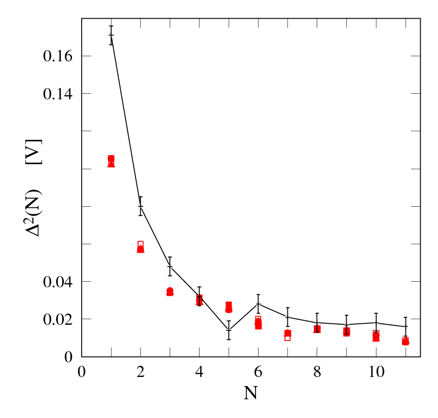
We now turn to the staircase-like addition spectra themselves. We plot the stair length in terms of the number of electrons, i.e., the right reservoir potential variation necessary to extract one electron. This gives the energy profile in terms of electron number. Experimentally observed addition spectra are given in Figs. 8 and 9 for two trap sizes corresponding to =0.5 and 0.3 volt respectively.


V Monte-Carlo simulations
In order to interpret the details of these experimental results, we have carried out Monte Carlo simulations of the addition spectra that correspond to the precise shape of the confining potential well in the experimental trap.
These MC simulations are based on the procedure described by Bedanov and Peeters.[14] In the low density limit, which is the regime attained here, the electrons occupy a small fraction only of the total area of the trap. They are (mostly) distinguishable and can be treated as classical particles. This simplification is also made by Peeters et al.
Our trap is not parabolic but its profile can be determined by finite elements calculation based on the known geometry (see Fig.3). Indoing so, we have attempted to reproduce as accurately as possible the pyramidal shape of the SET island. We used in the MC simulations values of the confining potential profile computed for a finite number of nodes whereas Peeters et al. use an analytic form. To find the electrostatic energy of an electron at coordinate in the trap, we fit the potential profile around by a 2D parabola between the three closest nodes of the calculated profile.
In order to check our computational procedure, we have reproduced Bedanov and Peeters’ results for a parabolic trap. We discretise the parabolic potential with the same number of nodes as with the actual potential for our cell. We then perform the same MC simulations to find the energy and the configuration of a known number of electrons in the trap. Our results, shown in Fig.10, fall very well in line with the published results, those of Ref.[14] and the more recent results of Kong et al. [36] The small systematic difference of 0.75 % seen in Fig.10 may be due to the discretisation of the confinement potential. We believe that it does not affect the global results and that our simulation does find the true ground state configuration.
To make sure that our simulations are not noisier than Peeters et al.’s, we compare addition spectra. Once again, our results are in very good agreement with those in the literature, as shown in Fig.11.

Finally, we compare electronic configurations. The ground state of the configuration with 31 electrons is one of the most difficult to find due to the closeness of the first metastable state (the difference is only 0.004%). The result, shown in Fig.12, is once again in agreement with Peeters et al.’s. We thus are quite confident that our MC simulations lead to correct configurations and energies.

We now turn to the case of addition spectra in the actual (non-parabolic) trapping potential, for which we need the electron energy. This energy has two parts: an electrostatic part and the repulsion due to the Coulomb interaction. The electrostatic part can be attractive if electrons are in the trap or repulsive if the electrons are on the other side of the barrier (see Fig.3). The electron energy reads, discarding the kinetic energy term in Eq.(1):
| (4) |
where is the electrostatic energy, obtained by a finite elements calculation, the -th electron coordinate, and the electron charge. The second term represents the Coulomb energy between electrons. The bulk part of the energy comes from the trapping; only around 10 % of the total energy in Eq.(4) is due to the Coulomb interaction.
An electron leaves the trap when its energy overcomes the confining potential , which is the energy difference between the minimum and the energy at the barrier (see Fig.3). That is, a given configuration is stable as long as the average energy per electron remains lower than the confining potential:
| (5) |
This assumes that electrons have identical energies.
We first compute the evolution of the confining potential in terms of the potential applied to the reservoir. The contact potential must be taken into account: when the potentials applied to the SET electrode and to the reservoir electrode are and , the potentials used in the simulations are V on the SET electrode and left unchanged on the reservoir electrode. For electrons in the trap, we compute the total energy for different values of the reservoir potential. When the barrier too low - i.e. when the reservoir potential is too close to the threshold when the electron is about to escape - the Monte-Carlo simulations fail to find the ground state. The starting temperature in the simulations is too high and allows electrons to escape readily over the barrier. Using a lower starting temperature to circumvent the problem does not lead to the real ground state of the configuration. To resolve this issue we calculated the energy for values of the reservoir potential slightly lower than the escape threshold, for which the simulations did find the ground state, and extrapolated the results linearly to higher values of this potential.
Figure 13 shows the evolution of the confining potential and the average energy per electron for N=1, 3, and 5 in terms of the reservoir voltage. An electron leaves the trap when these curves intersect.
Figures 8 and 9 show the comparison between the outcome of these calculations and the experimental results for respectively =0.5 and =0.3 V. The size and the shape of the trap depend on and the results are significantly different. Different potential sweeps following a given corona discharge are shown on the same graph in Fig.8: the experiment gives quite reproducible results. The scatter on the experimental points is less than the uncertainty on the simulations. The observed addition spectra are quite reproducible as long as the cell is kept cold, below 1 K. When it becomes necessary to replenish the electron reservoir, the temperature is raised and a new corona discharge ignited. Then the distribution of stray charges changes and the addition spectra fine structure, which is quite sensitive to the potential profile, also changes.
The addition energy is well predicted for . For very few electrons (), the Monte-Carlo simulation yields a larger addition energy.
A recurrent feature of the observed spectra is a peak for followed by a trough for . Referring to the work of Güçlü et al. [41], this indicates that electrons order in shells and not on a triangular lattice, which would give a peak at . The corresponding trap frequency is GHz and the electronic density . These observations correspond to the phase diagram shown in Fig.1 according to which, at an electron temperature of 200mK, the cluster is radially oriented (formation of shells) but not orientationally oriented.
As a rule, the experimental addition energies are found smaller than the calculated ones, especially for low occupation number. This observation probably means that the Wigner island is in an excited configuration. Its energy is higher than that of the ground state; a lesser decrease of the barrier is required to extract one electron. On the contrary, higher values than the calculated ones remain unexplained (e.g., in Fig.8). The extraneous source of noise energy that seems to be present in the experiment possibly comes from the tight coupling with the SET. We have evidence that the SET backaction affects the temperature of the electrons in the island in a way that depends on the SET bias current, either heating or cooling with respect to the bath temperature. This effect is under study.
It is known from the moving pictures of vortex lines configuration in a superfluid rotating bucket by Williams and Packard [23] that the vortices tend to jump around randomly. In order to damp the vortex motions so that they could be photographed, the authors of Ref.[23] added 3He impurities to the 4He superfluid to bring in some dissipation. In our Wigner islands, no such dampener is introduced. Due to the extremely high mobility of electrons over helium, it is quite likely that the electronic configuration is also extremely unsteady.
VI Conclusion
We have studied the confinement of a small number of electrons in a trap over a liquid helium film. Stable configurations down to a single electron can be obtained reproducibly and their energy recorded with an SET readout. The experimental addition spectra compare well with those obtained in Monte Carlo simulations in a trapping potential directly derived from the cell geometry. Charges trapped in the dielectric parts of the sample modify only weakly the potential profile. The good agreement between actual experiments and MC simulations 1) confirms the validity of the model (and assumptions) used in the simulation, 2) shows that no uncontrolled, or unforeseen, feature plays a significant role in the physical system, 3) opens the way, once the problem of repeatability of addition spectra after corona discharges is solved, to more detailed studies of these Wigner islands, and, in particular, of orientational ordering.
Acknowledgements.
This work has been supported in part by Fonds National de la Science, grant ACI 2002-2140. It was started as a collaboration with the Royal Holloway College in the framework of the European Network HPRN-CT-2000 00157.References
- [1] E. Wigner, Phys. Rev. 46, 1002 (1934).
- [2] C. Grimes and G. Adams, Phys. Rev. Lett. 42, 795 (1979).
- [3] V. Shikin, Sov. Phys. Usp. 32, 452 (1989).
- [4] B. Tanatar and D. M. Ceperley, Phys. Rev. B 39, 5005 (1989).
- [5] X. Waintal, Phys. Rev. B 73, 075417 (2006).
- [6] A. Ghosal, A. Güçlü, C. Umrigar, D. Ullmo, and H. U. Baranger, Phys. Rev. B 76, 085341 (2007).
- [7] D. Stauffer and A. Fetter, Phys. Rev. 168, 156 (1968).
- [8] L. Campbell and R. Ziff, Phys. Rev. B 20, 1886 (1979).
- [9] A. Abrikosov, Soviet Phys. JETP 5, 1174 (1957).
- [10] D. Cribier, B. Jacrot, L. M. Rao, and B. Farnoux, Phys. Lett. 9, 109 (1964).
- [11] U. Essmann and H. Trauble, Phys. Lett. 24A, 526 (1967).
- [12] Y. E. Lozovik and V. I. Yudson, JETP Lett. 22, 11 (1975).
- [13] M. Shayegan, Topological Aspects of Low Dimensional Systems (Springer-Verlag, Berlin, 1999), p. 1, Les Houches Summer School, Session LXIX, eds. A. Comtet, T. Jolicoeur, S. Ouvry, and F. David.
- [14] V. Bedanov and F. Peeters, Phys. Rev. B 49, 2667 (1994).
- [15] V. Schweigert and F. Peeters, Phys. Rev. B 51, 7700 (1995).
- [16] A. Koulakov and B. Shklovskii, Phys. Rev. B 57, 2352 (1998).
- [17] R. Egger, W. Hausler, C. Mak, and H. Grabert, Phys. Rev. Lett. 82, 3320 (1999).
- [18] A. Filinov, M. Bonitz, and Y. E. Lozovik, Phys. Rev. Lett. 86, 3851 (2001), also, M. Bonitz et al. arXiv:0801.0754 (2008).
- [19] A. Harju, S. Siljamäki, and R. Nieminen, Phys. Rev. B 65, 075309 (2002).
- [20] S. Reimann and M. Manninen, Rev. Mod. Phys. 74, 1283 (2002).
- [21] M. Saint-Jean, C. Even, and C. Gutmann, Europhys. Lett. 55, 45 (2001).
- [22] I. Gregorieva, W. Escoffier, J. Richardson, L. Vinnikov, S. Dubonos, and V. Oboznov, Phys. Rev. Lett. 96, 077005 (2006).
- [23] G. Williams and R. Packard, Phys. Rev. Lett. 33, 280 (1974).
- [24] U. Parts et al., Europhys. Lett. 31, 449 (1995).
- [25] G. Papageorgiou et al., Appl. Phys. Lett. 86, 153106 (2005).
- [26] D. Pfannkuche, V. Gudmundson, and P. Maksym, Phys. Rev. B 47, 2244 (1993).
- [27] E. Anisimovas and A. Matulis, J. Phys.: Condens. Matter 10, 601 (1998).
- [28] K. Balzer, C.Nölle, M. Bonitz, and A. Filinov, J. Phys.: Conference Series 35, 209 (2006).
- [29] N. Simonović, Few-Body Systems 38, 139 (2006).
- [30] See S.M. Reimann, M. Koskinen, and M. Manninen, Phys. Rev. B, 62, 8108 (2000) and references therein.
- [31] B. Reusch, W. Hausler, and H. Grabert, Phys. Rev. B 63, 113313 (2001).
- [32] V. Schweigert, F. M. Peeters, and P. S. Deo, Phys. Rev. Lett. 81, 2783 (1998).
- [33] B. Szafran, F. Peeters, S. Bednarek, and J. Adamowski, Phys. Rev. B 69, 125344 (2004).
- [34] Quoted by Saint-Jean et al. [21].
- [35] Y.-J. Lai and L. I, Phys. Rev. E 60, 4743 (1999).
- [36] M. Kong, B. Partoens, and F. Peeters, Phys. Rev. E 65, 046602 (2002).
- [37] M. Kong, B. Partoens, and F. M. Peeters, Phys. Rev. E 67, 021608 (2003).
- [38] M. Saint-Jean and C. Gutmann, J. Phys.: Condens. Matter 14, 13653 (2002).
- [39] S. Tarucha, D. G. Austing, T. Honda, R. van der Hage, and L. P. Kouwenhoven, Phys. Rev. Lett. 77, 3613 (1996).
- [40] L. Kouvenhoven, D. Austing, and S. Tarucha, Rep. Prog. Phys. 64, 701 (2001).
- [41] A. Güçlü, A. Ghosal, C. Umrigar, and H. U. Baranger, Phys. Rev. B 77, 041301 (2008).
- [42] D. Fisher, B. Halperin, and P. Platzman, Phys. Rev. Lett. 42, 798 (1979).
- [43] M. Dykman, P. M. Platzman, and P. Seddighrad, Phys. Rev. B 67, 155402 (2003).
- [44] M. Lea, P. Frayne, and Y. Mukharsky, Fortschr. Phys. 48, 1109 (2000).
- [45] E. Y. Andrei, ed., Two Dimensional Electron Systems on Helium and Other Cryogenic Substrates (Kluwer Academic, Dodrecht, 1997).
- [46] K. Shirahama, S. Ito, H. Suto, and K. Kono, J. Low Temp. Phys. 101, 439 (1995).
- [47] E. Rousseau, D. Ponarine, E. Varoquaux, and Y. Muhkarsky, J. Low Temp. Phys. 148, 193 (2007).
- [48] E. Rousseau, Ph.D. thesis, Université Paris XI (2006), http://tel.archives-ouvertes.fr/tel-00250371/fr/.
- [49] P. Glasson, G. Papageorgiou, K. Harrabi, and et al., J. Phys. Chem. Sol. 66, 1539 (2005).
- [50] M. Devoret and R. Schoelkopf, Nature 406, 1039 (2000).
- [51] K. Likharev, Nano et Micro Technologies 3 (2003).