[5cm]
YITP-08-61
AP-GR-61
OCU-PHYS-302
APCTP Pre2008-05
Solving the Inverse Problem with Inhomogeneous Universes
Abstract
We construct the Lemaître-Tolman-Bondi (LTB) dust universe whose distance-redshift relation is equivalent to that in the concordance cold dark matter (CDM) cosmological model. In our model, the density distribution and velocity field are not homogeneous, whereas the big-bang time is uniform, which implies that the universe is homogeneous at its beginning. We also study the effects of local clumpiness in the density distribution as well as the effects of large-scale inhomogeneities on the distance-redshift relation, and show that these effects may reduce the amplitude of large-scale inhomogeneities necessary for having a distance-redshift relation that is the same as that of the concordance CDM universe. We also study the temporal variation of the cosmological redshift and show that, by the observation of this quantity, we can distinguish our LTB universe model from the concordance CDM model, even if their redshift-distance relations are equivalent to each other.
1 Introduction
cold dark matter (CDM) models have achieved wide acceptance as concordance models due to the results of observations over the last decade. In particular, cosmic microwave background (CMB)[1] and supernovae (SNe)[2, 3, 4, 5] observations have played critical roles in this acceptance. The isotropy of our universe is strongly supported by the CMB observations. Thus, if we assume that our universe is homogeneous, results from SNe observation suggest that the volume expansion of our universe is accelerating. The accelerating expansion of a homogeneous and isotropic universe means the existence of exotic energy components, the so-called dark energy, within the framework of general relativity (GR). If we consider dark energy as a perfect fluid, it has negative pressure. One of the candidates for dark energy is the cosmological constant. However, there are several crucial problems regarding the existence of the cosmological constant or other dark energy candidates (see, for example, Ref.\citenKolb:2007gb). No one knows the origin of dark energy and there has not yet been a conclusive illustration of dark energy.
There are other possibilities that explain the CMB and SNe observations. observations. In the above logic, we have imposed two assumptions. One is validity of GR at all cosmological scales. The other is the homogeneity of our universe. Hence, in order to describe the observational results without dark energy, we need to discard GR or homogeneous models of the universe. In this paper, we attempt to describe the observational results without dark energy or any modification of gravitational theory, but with inhomogeneous universe models.
The basic idea is that we are in a large underdense region, i.e., a large void; we reject the Copernican principle, which states that we live at a typical position in the universe. Pioneering works include those Zehavi et al.[7] in 1998 and Tomita[8, 9, 10] in 2000 and 2001. Zehavi et al. analyze early SNe data and suggested that such a large void might exist around us without dark energy. Tomita proposed the void universe model and discussed the possibility of explaining the observed magnitude-redshift relations of SNe [8, 9, 10]. There are several works in the same direction [11, 12, 13, 14, 15, 16, 17, 18] (See also the reviews.[19, 20, 21]). In these works, Lemaître-Tolman-Bondi (LTB) solutions[22, 23, 24] are often employed. LTB solutions are exact solutions of the Einstein equations, which describe the dynamics of a spherically symmetric dust fluid and are useful for constructing universe models with a spherically symmetric void.
Recently, several authors have discussed the possibility of explaining the CMB observations[25, 26, 27]. They used asymptotically homogeneous LTB models and reported that these models may be consistent with the observed CMB anisotropy. In order to obtain more precise predictions on whether we are located near the center of a large void, we need to study the evolution of nonspherical density perturbations in the LTB universes[28]. Other methods of observationally investigating the inhomogeneity of our universe have been proposed in several papers [29, 30, 31, 32, 33].
The aforementioned works are very important for strengthening the observational foundation of physical cosmology. At present, the Copernican principle is not based on sufficient observational facts. However, by virtue of the recently improved observational technologies, we might reach the stage at which we are able to investigate through observation whether our location in the universe is unusual or not . In order to test inhomogeneous universe models by observations, it is important to know the types of inhomogeneous universe models that can be used to explain current observations, and to reveal what predictions are given by these universe models. This is the subject of this paper.
The inverse problem using LTB universe models is a useful method for investigating the possibility of explaining observational results with inhomogeneities in the universe [34, 12, 14, 35]. LTB dust solutions contain three arbitrary functions of the radial coordinate: the mass function , the big-bang time and the curvature function , and the inverse problem means determining , and so that a given distance-redshift relation is realized on the past light-cone of an observer. In order to specify the three arbitrary functions, we need three conditions. One of these conditions corresponds to the choice of the radial coordinate and thus has no physical meaning. Hence, one more condition in addition to the distance-redshift relation is necessary.
Iguchi et al.[12] showed that the distance-redshift relation in the standard CDM model can be reproduced in LTB dust universe models. When they solved the inverse problem, they imposed two kinds of the additional condition: one is a uniform big-bang time and the other is a vanishing curvature function . It should be noted that their models failed to reproduce the distance-redshift relation for . The reason why they could not continue their computation beyond is the existence of the “critical point” discussed by Vanderveld et.al[35]. They reported the difficulty in solving the inverse problem and concluded that it is unlikely that a solution to the inverse problem can be found in all the redshift domain. However, Tanimoto and Nambu recently solved the inverse problem in all the redshift domain with a nonuniform [36]. In this paper, we show that it is possible to obtain a solution to the inverse problem with the condition of the uniform big-bang time . 11 1 Mustapha et al.[34] proposed the following theorem :Subject to the conditions of Appendix B in Ref.\citenMustapha:1998jb for any given isotropic observation of apparent luminosity and number count with any given source evolution function and total density over source number density , a set of LTB functions can be found to make the LTB observational relations fit the observations. It is nontrivial whether the same statement holds for any given set of some quantities different from , , and . In this paper, the big-bang time is given as one of the quantities. Thus, the situation is different from the case in Ref.\citenMustapha:1998jb. In terms of perturbation theory, the inhomogeneity of the big-bang time corresponds to the decaying mode. The condition of uniform big-bang time might guarantee the consistency of the present model with the inflationary scenario, since a universe that experiences inflation is almost homogeneous immediately after the inflationary period is over.
In this paper, we also discuss the effects of local clumpiness. In addition to the effect of the large-scale void structure, small-scale clumpiness may affect the observed distance-redshift relation. If there are clumpy objects such as galaxies in the foreground of light sources, data for the apparent luminosities of these sources are often contaminated with gravitational lensing or absorption. For this reason, supernova teams specifically search for objects with a minimum amount of intervening material in the foreground[37, 21]. The observed sources might be biased by this selection, since the light of the observed sources might propagate in a lower-density region of our universe. The simplest way to take account of this effect is to introduce the so-called smoothness parameter , which is the ratio of the smoothly distributed matter density except for clumps to the mean energy density for all matter, assuming that the energy density on the paths of observed light rays is given by [38, 39, 40]. Tomita has studied the effects of small-scale clumpiness in a local void model by introducing the smoothness parameter . In this paper, we also investigate the corresponding effects by introducing .
The time derivative of the cosmological redshift is a very important observable quantity in distinguishing LTB models from concordance CDM universe models. We study it and show that it gives a criterion for observationally deciding whether the universe is described by an LTB model with uniform big-bang time.
This paper is organized as follows. In §2, we briefly review LTB dust universes and list basic equations that we have to solve. The temporal variation of the cosmological redshift of comoving sources is discussed in §3. Then, we show details of our numerical method, particularly, focusing on singular points of the equations at the center and the critical point in §4. Numerical results are given in §5. Section6 is devoted to a summary and discussion.
Throughout this paper, we use the unit of , where and are the speed of light and the gravitational constant, respectively.
2 Basic equations
2.1 LTB dust universe
LTB solutions are exact solutions to the Einstein equations, which describe the dynamics of a spherically symmetric dust fluid and whose line element is written in the form
| (1) |
where is an arbitrary function of the radial coordinate . The LTB solutions include homogeneous and isotropic universes as special cases; in this case, is a constant called the curvature parameter in the appropriate gauge, and thus we call it the curvature function. The stress-energy tensor of the dust is given by
| (2) |
where is the rest mass density of the dust and is the 4-velocity of a dust particle. The Einstein equations lead to the equations for the areal radius and the rest mass density ,
| (3) |
and
| (4) |
where is an arbitrary function of the radial coordinate . We assume that is nonnegative and that is monotonic with respect to , i.e., .
Following Tanimoto and Nambu [41], the solution to Eqs. (3) and (4), which represents the expanding universe, is written in the form
| (5) | |||||
| (6) |
where is an arbitrary function of the radial coordinate . The function is defined as
| (7) |
is analytic in the domain . Some characteristics of the function are given in Appendix A and Ref.\citenTanimoto:2007dq. We can easily see from the above equations that the areal radius vanishes at . Thus, the function is called the big-bang time.
Following Refs.\citenEnqvist:2006cg and \citenEnqvist:2007vb, we define the local Hubble function by
| (8) |
and the density-parameter function of dust as
| (9) |
In LTB universes, we can define another expansion rate of the spatial length scale, the so-called longitudinal expansion rate, by
| (10) |
In the case of homogeneous and isotropic universes, agrees with . Thus, if we can measure the difference between and , it can be used as an indicator of the inhomogeneity in the universe[29].
2.2 Conditions and equations to determine arbitrary functions
As shown in the preceding subsection, the LTB solutions have three arbitrary functions: , and . We have one degree of freedom to rescale the radial coordinate . To fix one of the three functional degrees of freedom corresponds to fixing the gauge freedom of this rescaling, and it will be shown later how to fix it. The remaining two functional degrees of freedom are fixed by imposing the following physical conditions.
- •
Uniform big-bang time .
- •
The angular diameter distance is equivalent to that in the CDM universe in all the redshift domain except in the vicinity of the symmetry center in which is appropriately set so that the regularity of the spacetime geometry is guaranteed.
Here we stress that it is our primary purpose to find an LTB model that fits the observed distance-redshift relation well. Thus, it does not matter that the distance-redshift relation does not agree with that of CDM model only in the vicinity of the symmetry center.
In order to determine and from the above conditions, we consider a past-directed outgoing radial null geodesic that emanates from the observer at the center. This null geodesic is expressed in the form
| (11) | |||||
| (12) |
where is an affine parameter.
We assume that the observer is always located at the symmetry center and observes the light ray at . In order to fix the gauge freedom to rescale the radial coordinate , we adopt the light-cone gauge condition that the relation
| (13) |
is satisfied along the observed light ray.
Then the basic equations to determine and are given as follows:
- 1.
Null condition
By virtue of the light-cone gauge condition, the null condition on the observed light ray takes the very simple form of
(14) - 2.
Definition of redshift
The redshift is defined by
(15) where is the tangent vector of the null geodesic that corresponds to the observed light ray and the dot represents differentiation with respect to the affine parameter . By using the freedom to multiply the affine parameter by a constant, we can write, without loss of generality,
(16) where
(17) and we have used the gauge condition (13) in the first equality. In this normalization, the affine parameter is dimensionless.
- 3.
Geodesic equation
One of the geodesic equations for the radial null geodesic is given by
(18) where we have used the null condition (14).
- 4.
Dyer-Roeder equation for the angular diameter distance
As mentioned, in order to fix the remaining functional freedom, we assume the angular diameter distance . Then the Dyer-Roeder equation
(19) gives us one of the equations to determine the arbitrary functions of LTB universe models, where is the smoothness parameter mentioned in §1. The derivation for this equation is given in Appendix B. is the mass ratio of the smoothly distributed components of matter to all the components, and it may vary with time due to the formation of structures in the real universe. Therefore, in this paper, we assume that is an input function of the cosmological redshift .
3 Temporal variation of the cosmological redshift
The temporal variation of the cosmological redshift will give us crucial information about the acceleration of cosmic volume expansion or inhomogeneities in our universe[42].
3.1 Homogeneous and isotropic universe
The line element of homogeneous and isotropic universes is given by
| (28) |
where for a closed universe, for a flat universe and for a open universe. In this subsection, we assume that the universe is filled with dust and dark energy characterized by the linear equation of state , where is the pressure, is the energy density and is a constant less than . We assume that the energy densities of both dust and dark energy are nonnegative.
The Einstein equations lead to
| (29) |
where is the scale factor at , and and are the density parameters of the dust and the dark energy, respectively. Note that, by assumption, both and are nonnegative. As is well known, the cosmological redshift of a light signal emitted from a comoving source is given by
| (30) |
where is the time when the light is emitted from the source. The temporal variation of of a comoving source is then given by
| (31) |
where and is the Hubble parameter when the light is emitted from the source. Substituting Eq. (29) into the above equation, we have
| (32) |
Note that, is nonnegative, whereas is nonpositive due to the assumption . Thus, if the dust is a dominant component of the universe, i.e., , then is negative. By contrast, in the case of a universe dominated by dark energy, i.e., , then is positive. Therefore, the measurement of the temporal variation of the cosmological redshift will give us crucial knowledge about the equation of state if the universe is homogeneous and isotropic.
3.2 LTB universe
In order to obtain the time derivative of the cosmological redshift in LTB universe models, we consider another past-directed outgoing radial null geodesic that is infinitesimally close to the null geodesic considered in the preceding section,
| (33) |
where and denote the null geodesic with the initial condition at , which was considered in the preceding section. We set the affine parameter so that the cosmological redshift is given by
| (34) |
where the subscript “b” denotes the value evaluated on the null geodesic . Thus, we have
| (35) |
Substituting Eq. (33) into Eq. (18), and taking the first order of and , we have
| (36) |
Another equation is given by the null condition,
| (37) |
The initial conditions for these equations are given by
| (38) | ||||
| (39) | ||||
| (40) |
The temporal variation of the cosmological redshift of a comoving source is given by
| (41) |
where the infinitesimal quantity satisfies the equality
| (42) |
From Eqs. (33), (34), (41) and (42), we have, up to the first order of ,
| (43) |
Thus, we have the derivative of the cosmological redshift with respect to the time of the observer as a function of the affine parameter,
| (44) |
Since we also obtain simultaneously, we have the relation between and . In order to solve the differential equations (36) and (37), we need to know , and , which are given in Appendix D. Using Eq.(94), Eq.(37) can be solved as
| (45) |
4 Singularity at the center and critical point
4.1 Resolving singularity at the center
Suppose that the reference angular diameter distance is exactly the same as that of the concordance CDM model with , where is the density parameter of the cosmological constant. Then, as shown in Appendix E, once is given, the set of solutions for the differential equations (20)-(24) is uniquely determined. Vanderveld et al.[35] reported that many of the inhomogeneous models that mimic observations of an accelerating universe contain a weak singularity at the symmetry center. This singularity is too weak to make the spacetime geodesically incomplete, and thus we may accept these models as being effective.
On the other hand, the accuracy of observations in the low-redshift domain is not sufficient to uniquely determine the distance-redshift relation. Thus, we need to assume the redshift dependence of the angular diameter distance in the low-redshift domain. If the model is preferred, we may assume the following input angular diameter distance ,
| (46) |
where is a positive constant, whereas and are the angular diameter distances in the isotropic and homogeneous universe with and , respectively. is almost the same as the angular diameter distance of the CDM model for , whereas, in the vicinity of the symmetry center, is almost the same as that of the homogeneous and isotropic universe with . It should be noted that is equal to and can be regarded as a parameter to specify the LTB universe model.
Also note that if our vicinity is described well by the very smooth LTB model, the distance-redshift relation does not agree with that of the concordance CDM model in the low-redshift domain. Nambu and Tanimoto have shown that the Maclaurin series of for the LTB model with a regular symmetry center agrees with the homogeneous and isotropic dust-filled universe up to . The angular diameter distance (4.1) is one of the simplest assumptions that ensures the regularity at the symmetry center and agrees with that of the concordance CDM model in the high-redshift domain.
4.2 Critical point
The differential equation (23) has a singular point at which vanishes. Following Ref.\citenVanderveld:2006rb, we call this point the critical point and denote the cosmological redshift at the critical point by . We can require that the value of should vanish at the critical point so that the solution is regular at this point. This gives a constraint on the free parameter .
The symmetry center is another regular singular point of the differential equations (20)-(24). The Runge-Kutta method, which we have used, is generally unstable for solving ordinary differential equations toward a regular singular point from a regular point, and thus we start the numerical integration from these regular singular points; we numerically integrate the equations from the symmetry center but not to the critical point , and we also integrate them from the critical point but not to the symmetry center . Instead, specifying and the values of , and at the critical point , we numerically integrate the differential equations outward from the symmetry center and inward from the critical point to the matching point located in the domain between these singular points.
If we fail to choose appropriate values of and values of , and at the critical point , the resultant solutions are discontinuous at . Thus, we have to search for the appropriate initial values for , and , and at the critical point so that the following matching conditions are satisfied:
| (47) |
Note that if the above conditions hold, the smoothness of the solutions is also guaranteed, since the equations for these functions are first-order differential equations.
5 Numerical results
We have solved Eqs. (20)-(24) by using the numerical procedure described in the previous section. In the following subsections, we express , , , , and as functions of the cosmological redshift . We also express the time derivative of the cosmological redshift as a function of the cosmological redshift itself together with that of the concordance CDM universe with .
5.1 Results without local clumpiness
In this subsection, we assume . As mentioned above, the solution is uniquely given by our numerical procedure if the value of in Eq. (46) is fixed. First, we show and as functions of in Figs. 1 and 2, respectively. The results do not strongly depend on the value of except when .
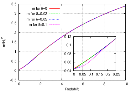
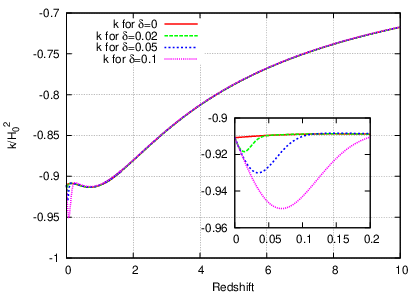
In order to determine the physical properties of the solution, we depict , , and and , respectively, as functions of in Figs. 3-5. We can see from these figures that the resultant inhomogeneity is a large-scale void structure.
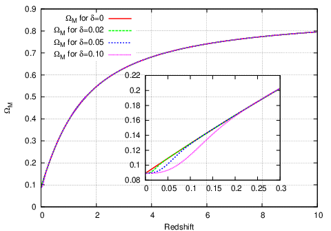
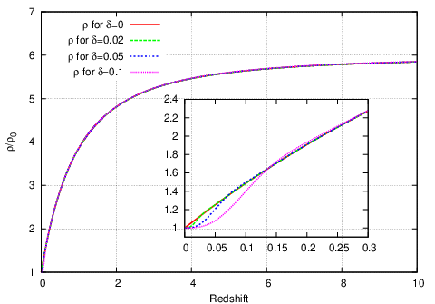
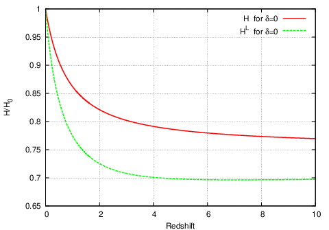
We note that in homogeneous and isotropic universes, whereas and are different from each other by about 10% for in the inhomogeneous case depicted in Fig. 5. This result means that, in order to fit the distance-redshift relation of the LTB model with observations that almost agree with that predicted by the concordance CDM universe with , the scale of the inhomogeneity should be at least a few Gpc.
5.2 Results with local clumpiness
In this subsection, we fix the value of as 0 and study the effects of local clumpiness. The vanishing implies that agrees with the angular diameter distance of the concordance CDM model, and thus the weak singularity appears at the symmetry center.
In the early universe, the matter distribution might have been smooth, whereas it might have been highly clumpy after the structures formed. The simplest way to take account of the effects of local clumpiness and the growth of structures is to introduce a -dependent smoothness parameter , which represents the fraction of matter spreading out almost homogeneously. The light rays propagating from standard candles to us pass through regions filled with matter of energy density .
At present, the -dependence of is still unclear. However, as the structures grow, the spreading-out component of the mass might decrease, and therefore might be an increasing function of . Furthermore, there might be a typical redshift at which almost all of the mass components form clumpy structures. This typical redshift will depend on the scenario of structure formation. For , the light rays might propagate to us through almost empty regions. Thus, we assume the following form for the smoothness parameter :
| (48) |
A bundle of light rays propagating through a region where is called a filled beam, while a bundle of light rays propagating through a region where is called an empty beam. Thus, all bundles of light rays are empty beams in the model of . In the case of the empty beam, the angular diameter distance does not have a maximal value, and it is clear that the distance in the case cannot fit the distance in the CDM universe in all the redshift domain. The results depend on the value of as shown in Figs. 69. The resultant inhomogeneity is also a large-scale void structure.


We show that it is possible to reduce the amplitude of the large-scale inhomogeneity by choosing an appropriate value of . In Fig. 10, values of and are depicted as functions of for . In this case, the difference between and is a few percent when , and the amplitude of the inhomogeneity is smaller than that depicted in Fig. 5. This means that the appropriate value of the redshift that characterizes the period of local clumpiness formation may suppress the size of the void by a few Gpc. In our model, this appropriate value of the redshift is given by . In the region of our model with , the geometry of the universe is almost the same as that of the isotropic and homogeneous universe.

5.3 Time variation of the redshift
We have shown in the preceding subsections that it is possible to construct the LTB universe model with the same distance-redshift relation as that of the concordance CDM model. Thus, it is very important to study how to observationally distinguish these two models from each other. Here, we show that the temporal variation of the cosmological redshift is a useful observational quantity. In Fig. 11, we depict the derivative of the cosmological redshift with respect to the time of the observer at the symmetry center as a function of the cosmological redshift itself.
As can be seen from this figure, is positive for in the case of the concordance CDM model, while it is negative for all in the LTB universe models with the uniform big-bang time. Therefore, if we observe whether is positive or negative for , we can distinguish our LTB model from the concordance CDM model. From Eq. (32), we have for the concordance CDM model, and thus, the variation of the cosmological redshift in one year is /75 km/s/Mpc). Thus, over ten years, is larger than for the concordance CDM universe model, and this value will become observable in the near future as a result of technological innovations[43, 44].

6 Summary and discussion
In this paper, we have attempted to solve the inverse problem to construct an LTB universe model that has the same distance-redshift relation as that of the concordance CDM model with , and we obtained solutions by numerical integration. In the present study, assuming an inflationary period in the early universe, we have restricted ourselves to models with uniform big-bang time, and the resultant universe model has a very large void whose symmetry center is at the observer’s position. We have also studied the effects of local clumpiness by introducing the smoothness parameter , and have shown that the local clumpiness may reduce the amplitude of the large-scale inhomogeneity of the void. Our results imply that it is possible to construct an inhomogeneous but isotropic universe model with a distance-redshift relation that agrees quite well with the observational data of the distance-redshift relation.
Our LTB universe model is regarded as an unnatural model from the viewpoint of the Copernican principle, because the observer stands exactly at the center of the isotropic universe. The extent to which we can separate ourselves from the center and remain consistent with current observations is discussed in Refs.\citen2000ApJ…529…38T and \citen2000ApJ…529…26T,Tomita:2000rf,Alnes:2006pf,Alnes:2006uk. The strictest limit is given by Alnes and Amarzguioui in Ref.\citenAlnes:2006pf as 15 Mpc from the observation of CMB. This value is much smaller than the cosmological scale, and thus we should remain at a special position if the void universe is real. However, no observational data has yet been reported that entirely excludes inhomogeneous universe models. Therefore, it is important to know the type of inhomogeneous universes that can explain current observations and to propose observational methods for testing inhomogeneous universe models.
In this paper, we have also studied the temporal variation of the distance-redshift relation in our LTB universe model whose distance-redshift relation is the same as the concordance CDM model with . The result implies that if we can observe the time derivative of the cosmological redshift with sufficient accuracy, we can distinguish our LTB model from the concordance CDM universe model. Innovations in observational technology might provide us with data on the time derivative of the cosmological redshift in the near future [31, 43, 44].
Finally, we should note that if we ignore the inflationary paradigm, the functional freedom of the big-bang time is returned, and we might be able to construct an LTB universe model with the same redshift-distance relation and, furthermore, the same as those of the concordance CDM model by choosing an appropriate big-bang time [31]. However, in this case, we may need an other mechanism to explain the results in CMB observations and other cosmological problems than the standard cosmology starting from the inflation. This will be the subject of a future work and will be discussed elsewhere.
Acknowledgements
We are grateful to M. Tanimoto and Y. Nambu for helpful discussions and comments. This work was supported in part by a JSPS Grant-in-Aid for Scientific Research (B), No. 17340075.
Appendix A Characteristics of the Function
From Eqs. (3) and (5), the function is a solution of the following nonlinear differential equation:
| (49) |
We can easily see that is also a solution of Eq. (49). This solution is not equivalent to since from Eq. (7). It is verifiable by Eq. (7) that
| (50) |
is a root of the equation . In other words, the solutions and agree with each other at (See Fig. 12).
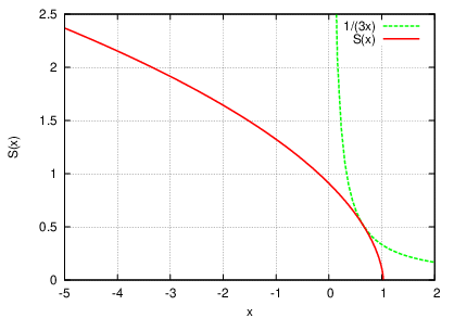
Let us consider the behaviour of a solution that is regular in the neighborhood of . Expanding around , we have
| (51) |
Substituting this expression into Eq. (49), we have, from the zeroth order of ,
| (52) |
and, from the first order of ,
| (53) |
Therefore, a solution that is regular at should satisfy . This result also means that is a unique solution that is regular at .
Next, we consider a solution that satisfies . Expanding around , we have
| (54) |
Substituting this expression into Eq. (49), we find, from the zeroth order of , that
| (55) |
Then, we have
| (56) |
Therefore, the derivative of at is unique. This result implies that the solutions and have the same gradient at . The first order of in Eq. (49) is automatically satisfied. From the second order, we have
| (57) |
There are two roots of the above equation, where
| (58) |
This fact means that there are at least two solutions of Eq. (49) with the same value and the same derivative at . The root corresponds to the solution whereas the other root corresponds to the solution . Since we have
| (59) |
and since and , we have
| (60) | |||||
| (61) |
Eventually, we obtain the differential equation for as
| (62) | |||||
| (63) |
Appendix B Dyer-Roeder Equation
Let us consider a bundle of light rays whose sectional area is given by . The expansion rate of along the ray is defined by
| (64) |
where the dot denotes differentiation with respect to an affine parameter of the ray bundle. Then the evolution of is given by [49]
| (65) |
where is a tangent vector of the light ray, and is the shear factor defined by
| (66) |
Substituting Eq. (64) into Eq. (65), we have
| (67) |
Let us assume that the light beam remains far away from clumps and that the contribution of in Eq. (67) is negligible [38, 39, 40]. In addition, we assume that the fraction of matter density that is smoothly distributed is given by , namely, the energy density on the ray is given by . As mentioned in §1, is the so-called smoothness parameter. Then, Eq. (67) reduces to
| (68) |
where we have used the Einstein equation with the energy momentum tensor (2).
Since the relation between the angular diameter distance and is given by
| (69) |
we obtain
| (70) |
When is given as a function of redshift , we can rewrite the above equation in the form of Eq. (19).
Appendix C Derivation of Basic Equations
From Eq. (16), we have
| (71) |
This is identical to Eq. (22). From Eq. (26), we obtain
| (72) |
as Eq. (23). Using , Eq. (19) can be written as Eq. (24):
| (73) |
The remaining task is the derivation of Eqs. (20) and (21) from Eqs. (14) and (18). Differentiating Eq. (5) with respect to , we have
| (74) | |||||
Substituting Eqs. (74) and (16) into Eq. (14)Cwe have
| (75) |
where
| (76) | |||||
| (77) | |||||
| (78) | |||||
| (79) |
Appendix D (∂ r 2 R) b , and
We show how to calculate , and on the null geodesic that corresponds to the observed light ray. Let us consider the differentiation of the null condition (14) along the null geodesic with respect to as follows:
| (92) |
Using , we have
| (93) |
where is given by Eq. (81).
The expression for is given by differentiating Eq. (3) with respect to and as
| (94) |
where is given by Eq. (74).
Finally, is given by differentiating the null geodesic equation (18) with respect to the affine parameter . Namely,
| (95) |
The above equation leads to
| (96) |
where
| (97) | |||||
| (98) | |||||
| (99) |
Appendix E Initial Conditions at the Center without Distance Modification
From the null condition, we have near the center. Thus we must have in order that the metric (1) is regular at the center. Therefore, from Eq. (4), should be given by
| (100) |
for the finiteness of at the center. Thus, we have
| (101) |
Hereafter, the subscript describes the initial value at the center. Obviously, . The remaining initial values are , and . In addition, the initial value of should also be determined.
Since
| (102) |
near the center, Eqs. (3), (4) and (5) are given by
| (103) |
| (104) |
| (105) |
where
| (106) |
Equation (104) can be rewritten as
| (107) |
where
| (108) | |||||
| (109) |
Once we fix the value of at the symmetry center, , or equivalently , is fixed by Eq. (107). and are related to by Eqs. (103) and (109). is given as the solution of Eq. (105). The remaining initial value is . Differentiating Eq. (3) with respect to , we have
| (110) |
The above equation becomes
| (111) |
at and . Using this equation, from Eqs. (16) and (18), we obtain
| (112) |
Thus, we have
| (113) |
References
- [1] D. N. Spergel et al., Astrophys. J. Suppl. 148 (2003) , 175.
- [2] A. G. Riess et al. [Supernova Search Team Collaboration], Astron. J. 116 (1998), 1009.
- [3] S. Perlmutter et al. [Supernova Cosmology Project Collaboration], Astrophys. J. 517 (1999), 565.
- [4] R. A. Knop et al., Astrophys. J. 598 (2003), 102.
- [5] A. G. Riess et al., Astrophys. J. 607 (2004), 665.
- [6] E. W. Kolb, arXiv:0709.3102.
- [7] I. Zehavi, A. G. Riess, R. P. Kirshner and A. Dekel, Astrophys. J. 503 (1998), 483.
- [8] K. Tomita, Astrophys. J. 529 (2000), 38.
- [9] K. Tomita, Mon. Not. R. Astron. Soc. 326 (2001), 287.
- [10] K. Tomita, Prog. Theor. Phys. 106 (2001), 929.
- [11] M.-N. Celerier, Astron. Astrophys. 353 (2000), 63.
- [12] H. Iguchi, T. Nakamura and K. Nakao, Prog. Theor. Phys. 108 (2002), 809.
- [13] K. Bolejko, PMC Phys. A 2 (2008), 1.
- [14] D. J. H. Chung and A. E. Romano, Phys. Rev. D 74 (2006), 103507.
- [15] K. Enqvist and T. Mattsson, J. Cosmol. Astropart. Phys. 02 (2007), 019.
- [16] D. Garfinkle, Class. Quant. Grav. 23 (2006), 4811.
- [17] M. Kasai, Prog. Theor. Phys. 117 (2007), 1067.
- [18] T. Biswas and A. Notari, astro-ph/0702555.
- [19] M.-N. Celerier, astro-ph/0702416.
- [20] K. Enqvist, Gen. Rel. Grav. 40 (2008), 451.
- [21] T. Mattsson, arXiv:0711.4264.
- [22] G. Lemaitre, Gen. Rel. Grav. 29 (1997), 641.
- [23] R. C. Tolman, Proc. Nat. Acad. Sci. 20 (1934), 169.
- [24] H. Bondi, Mon. Not. R. Astron. Soc. 107 (1947), 410.
- [25] H. Alnes, M. Amarzguioui and O. Gron, Phys. Rev. D 73 (2006), 083519.
- [26] S. Alexander, T. Biswas, A. Notari and D. Vaid, arXiv:0712.0370.
- [27] J. Garcia-Bellido and T. Haugboelle, J. Cosmol. Astropart. Phys. 04 (2008), 003.
- [28] J. P. Zibin, arXiv:0804.1787.
- [29] C. Clarkson, B. A. Bassett and T. H.-C. Lu, \PRL101,2008,011301.
- [30] R. R. Caldwell and A. Stebbins, \PRL100,2008,191302.
- [31] J.-P. Uzan, C. Clarkson and G. F. R. Ellis, \PRL100,2008,191303.
- [32] K. Bolejko and J. S. B. Wyithe, arXiv:0807.2891.
- [33] T. Clifton, P. G. Ferreira and K. Land, arXiv:0807.1443.
- [34] N. Mustapha, C. Hellaby and G. F. R. Ellis, Mon. Not. R. Astron. Soc. 292 (1997), 817.
- [35] R. A. Vanderveld, E. E. Flanagan and I. Wasserman, Phys. Rev. D 74 (2006), 023506.
- [36] M. Tanimoto and Y. Nambu, private communication.
- [37] R. Pain et al., Astrophys. J. 577 (2002), 120.
- [38] R. Kantowski, Astrophys. J. 155 (1969), 89.
- [39] C. C. Dyer and R. C. Roeder, Astrophys. J. 180 (1973), L31.
- [40] R. Kantowski, Astrophys. J. 507 (1998), 483.
- [41] M. Tanimoto and Y. Nambu, Class. Quantum Grav. 24 (2007), 3843.
- [42] K. Lake, Phys. Rev. D 76 (2007), 063508.
- [43] C.-H. Li et al., Nature 452 (2008), 610.
- [44] Liske, J. et al., Mon. Not. R. Astron. Soc. 386 (2008), 1192.
- [45] H. Alnes and M. Amarzguioui, Phys. Rev. D 74 (2006), 103520.
- [46] H. Alnes and M. Amarzguioui, Phys. Rev. D 75 (2007), 023506.
- [47] K. Tomita, Astrophys. J. 529 (2000), 26.
- [48] K. Tomita, Prog. Theor. Phys. 105 (2001), 419.
- [49] R. Sachs, Proc. R. Soc. London, Ser. A 264 (1961), 309.