Developments in the evaluation of dependent matrix elements in
Developments in the evaluation of dependent matrix elements in at NNLO
Abstract
The full prediction of the inclusive radiative decay rate at NNLO requires a complete evaluation of missing charm quark mass dependent matrix elements. Recent developments in the on-going computations are reported and the current status is briefly overviewed.
1 Introduction
One interesting candidate process in the indirect search for non-standard physics is the rare inclusive decay [1]. Due to its low sensitivity to non-perturbative effects and, being a flavour-changing neutral current, its loop-suppression in the Standard Model (SM) stringent constraints on the parameter space of physics beyond the SM can be derived from both accurate measurements and precise theory predictions.
The latest measurements by BaBar, Belle and CLEO [2] have been combined by the Heavy Flavour Averaging Group (HFAG) [3] into the current world average (WA) for the branching ratio,
| (1) |
where a cut GeV has been imposed on the photon energy in the -meson rest frame. The first uncertainty corresponds to a combined statistical and systematical error, the second one is due to the theory input in the extrapolation of the measured branching ratio to the reference value , whereas the third one is connected to the subtraction of contamination. On the theory side, the expected size of next-to-next-to leading order (NNLO) QCD effects to the partonic decay is comparable with the overall experimental error of about 7% and therefore a complete SM calculation at this level of accuracy is clearly needed.
The recent theoretical estimate of the branching ratio at the NNLO level
| (2) |
was derived in [4] after a large part of the NNLO program has been finished and is in good agreement with the WA. The uncertainty here consists of four types of error added in quadrature: non-perturbative (5%), parametric (3%), higher-order (3%) and -interpolation ambiguity (3%).
Large logarithms of the form appear in QCD corrections to the partonic decay width and have to be resummed with renormalization-group techniques to get a reasonable prediction. Most suitably, this is done in the framework of an effective low-energy theory with five active quarks by integrating out the heavy electroweak and the top fields in the SM. As a consequence, local flavour-changing operators up to dimension six and Wilson coefficients appear in the resulting effective Lagrangian .
A few years ago, the next-to-leading order QCD corrections to the decay have been completed (see e.g. [5, 6] and references therein). The next-to-next-to leading order evaluation, which is a very complicated task, is currently under way and large parts are already finished. In general, three steps are required for a consistent calculation in the low-energy effective theory and in particular also at the NNLO level:
- 1.
Determination of Wilson coefficients at the electroweak scale by requiring equality of Green’s functions in the effective and full theory at leading order in (external momenta)/. To this precision, the matching of the four quark operators and the dipole operators at the two- and three-loop level, respectively, has been computed in [7, 8].
- 2.
Derivation of the effective theory Renormalization Group Equations (RGE) and computation of the operator mixing under renormalization by evolving the Wilson coefficients from down to the low scale using the anomalous dimension matrix up to . In the sectors and , the three-loop renormalization was found in [9, 10]. Results for the four-loop mixing of into were recently found by completing the anomalous dimension matrix [11].
- 3.
Calculation of on-shell matrix elements with single insertions of effective operators at to . This task is not completed yet, although a number of contributions is known. In [12, 13], the two-loop matrix element of the dipole operator together with the corresponding bremsstrahlung was determined, confirmed in [14] and subsequently extended to include the full charm quark mass dependence in [15]. Dominant contributions to the photon energy spectrum in the so-called large- approximation have been obtained in [16]. Using an expansion in the contributions to the two-loop matrix elements of and , as well as to the three-loop matrix elements and , were found in [17]. These results have been confirmed in [18] and, moreover, the full fermionic corrections beyond the large- approximation have been provided there.
The full matrix elements of and at constitute an important piece that is still missing. At NLO the choice of scale and scheme of constitutes the main source of uncertainty stemming from the fact, that these operators contain the charm quark and contribute for the first time at . Removing this ambiguity is therefore a NNLO effect in the branching ratio. So far, the full matrix elements of the and operators have been evaluated in the large limit, , and subsequently used for an interpolation to the physical range of [19] assuming some ad-hoc value at . This is the source of the aforementioned interpolation ambiguity in the current NNLO branching ratio estimate. Removing this uncertainty requires the calculation of at physical and involves the evaluation of hundreds of on-shell three-loop vertex diagrams with two scales and . Reducing this interpolation uncertainty is possible by computing the matrix elements at and thus fixing the endpoint of the interpolation. Both evaluations are currently being pursued. This paper is meant to describe the current status.
2 The matrix elements at NNLO
The effective low-energy theory, in which the calculation of at is performed, is given by the effective Lagrangian
| (3) | |||||
The first term corresponds to the usual QED-QCD Lagrangian for the light SM fields, the second term gives the local operator product expansion, are the matrix elements of the Cabibbo-Kobayashi-Maskawa matrix and is the Fermi coupling constant. The relevant physical operators are chosen as [23]
| (4) | |||||
where and stand for various products of Dirac and colour matrices.
As already mentioned, removing the interpolation uncertainty requires the calculation of matrix elements at the NNLO level. All appearing vertex diagrams have been generated, expressed through scalar diagrams that depend on the two mass scales and and finally reduced with Laporta’s algorithm to 476 master integrals. The latter can be evaluated using two different approaches: numerical solutions of differential equations or the Mellin-Barnes technique. The first method consists of writing down differential equations for the master integrals in their kinematical invariants and solving them numerically after an expansion about some limit has been taken to provide the startpoint for integration with high precision. This was already used in the calculation of double fermionic QCD corrections to the photon polarization function [20]. Moreover, in [21] this idea was also applied to determine the full mass dependence of the -production cross-section from light quarks at NNLO. The second approach is based on the Mellin-Barnes (MB) technique, where MB representations can be derived in an automatized way, analytically continued in and numerically integrated utilizing the package MB [22]. Both methods have been used to obtain the full fermionic corrections, extending the so far known massless case to include heavy and quark loops [18]. As a result, it turned out that while the charm quark contribution is well reproduced by the massless approximation, bottom quark loop insertions are overestimated by a large extent. For the remaining bosonic parts the IBP reduction is still under way.
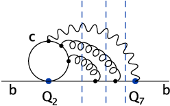
In the limit valuable information can be obtained from to fix the endpoint of the interpolation performed in [19]. A possible way of getting is by interfering the matrix elements of the operators with those of the dipole operator and cutting the resulting four-loop propagators selectively. The final state is required to contain at least one quark and one photon. Altogether, several hundreds of four-loop propagator-like diagrams are generated with up to five-particle cuts and subsequently reduced to about 200 master integrals that have to be evaluated. The massless cases among them have already been computed up to four-particle cuts using a Mellin-Barnes based method. For this task, Mellin-Barnes representations have been derived and numerically evaluated after performing the necessary phase space integrations. However, integrals containing massive lines from virtual -quarks require a different approach. The method we are currently using in this respect is again based on differential equations (DEQ), but it turns out to be more involved as compared to the virtual corrections at . As starting point for the expansion and integration of the system of DEQ we choose the large mass limit. Thus, boundary conditions are given by cut integrals in the large mass limit and can be evaluated with automatized diagrammatic expansions and phase space integration. Unfortunately, the usual approach of numerical integration up to the interesting kinematical point, to the on-shell limit in our case, suffers from divergences in the differential equations at both endpoints of the integration contour. This can be overcome by solving the system of DEQ with an expansion ansatz around the on-shell point. Comparison of the numerical integration at some point close to the on-shell kinematics with the expansion fixes the boundary conditions of the latter. In the case of logarithmic on-shell divergences, the integrals are regularized with a sufficient number of irreducible numerators and a change of the basis of master integrals.
The achievable accuracy of this method is, on the one hand, given by the depth of the expansions at the starting and ending points on the integration contour and, on the other, by the error pile-up during numerical integration.


.
Performing the numerical part with quadruple precision, a relative error of the order of at the on-shell point seems to be obtainable.
As a first attempt we study diagrams involving two- and three-particle cuts, which constitute the major part of the evaluation. Fig. 2 shows a plot of the term for one example integral. The expansion in the large mass limit has been performed up to 20 terms in whereas in the on-shell limit 12 terms have been taken into account. The numerical integration is performed starting at and the matching of the numerics and the on-shell expansion is done at . It is apparent, that both series converge nicely against the numerical points.
The first three terms of the expansion in the limit of of the integral in Fig. 2 are given by
The corresponding first few terms of the expansion around the on-shell kinematical point with read
3 Conclusions
An evaluation of the missing matrix elements at is essential for the reduction of the current uncertainty in the estimate of the branching ratio . Two different approaches are used and will eventually reduce or even remove the remaining -interpolation ambiguity that amounts to about 3%.
4 Acknowledgements
This work is supported by the Sofia Kovalevskaja Award of the Alexander von Humbold Foundation sponsored by the German Federal Ministry of Education and Research.
References
- [1] U. Haisch, arXiv:0706.2056 [hep-ph]; PoS KAON (2008) 056, arXiv:0707.3098;
- [2] S. Chen et al. [CLEO Collaboration], Phys. Rev. Lett. 87, 251807 (2001) [arXiv:hep-ex/0108032]; P. Koppenburg et al. [Belle Collaboration], Phys. Rev. Lett. 93, 061803 (2004) [arXiv:hep-ex/0403004]; B. Aubert et al. [BaBar Collaboration], Phys. Rev. Lett. 97, 171803 (2006) [arXiv:hep-ex/0607071].
- [3] E. Barberio et al. [Heavy Flavor Averaging Group (HFAG) Collaboration], arXiv:0704.3575 [hep-ex].
- [4] M. Misiak et al., Phys. Rev. Lett. 98 (2007) 022002
- [5] A. J. Buras and M. Misiak, Acta Phys. Polon. B 33 (2002) 2597
- [6] T. Hurth, Rev. Mod. Phys. 75 (2003) 1159
- [7] C. Bobeth, M. Misiak and J. Urban, Nucl. Phys. B 574 (2000) 291
- [8] M. Misiak and M. Steinhauser, Nucl. Phys. B 683 (2004) 277
- [9] M. Gorbahn and U. Haisch, Nucl. Phys. B 713 (2005) 291
- [10] M. Gorbahn, U. Haisch and M. Misiak, Phys. Rev. Lett. 95 (2005) 102004
- [11] M. Czakon, U. Haisch and M. Misiak, JHEP 0703 (2007) 008
- [12] K. Melnikov and A. Mitov, Phys. Lett. B 620 (2005) 69.
- [13] I. Blokland, A. Czarnecki, M. Misiak, M. Ślusarczyk and F. Tkachov, Phys. Rev. D 72 (2005) 033014.
- [14] H. M. Asatrian, A. Hovhannisyan, V. Poghosyan, T. Ewerth, C. Greub and T. Hurth, Nucl. Phys. B 749 (2006) 325; H. M. Asatrian, T. Ewerth, A. Ferroglia, P. Gambino and C. Greub, Nucl. Phys. B 762 (2007) 212.
- [15] H. M. Asatrian, T. Ewerth, H. Gabrielyan and C. Greub, Phys. Lett. B 647 (2007) 173
- [16] Z. Ligeti, M. E. Luke, A. V. Manohar and M. B. Wise, Phys. Rev. D 60 (1999) 034019
- [17] K. Bieri, C. Greub and M. Steinhauser, Phys. Rev. D 67 (2003) 114019.
- [18] R. Boughezal, M. Czakon and T. Schutzmeier, JHEP 0709 (2007) 072
- [19] M. Misiak and M. Steinhauser, Nucl. Phys. B 764 (2007) 62
- [20] M. Czakon and T. Schutzmeier, arXiv:0712.2762 [hep-ph].
- [21] M. Czakon, arXiv:0803.1400 [hep-ph].
- [22] M. Czakon, Comput. Phys. Commun. 175 (2006) 559
- [23] K. G. Chetyrkin, M. Misiak and M. Munz, Phys. Lett. B 400 (1997) 206 [Erratum-ibid. B 425 (1998) 414]