跳到论文正文
W Papers独立论文阅读器 arXiv:0807.0789 论文正文 计算阅读时间 · 0%
引用这篇论文根据当前论文元数据生成,正式投稿前建议核对。


License: arXiv.org perpetual non-exclusive license
arXiv:0807.0789v1 [hep-th] 06 Jul 2008

Wave Functions and Yukawa Couplings in Local String Compactifications

Preprint: DAMTP-2008-33
Joseph P. Conlon Affiliation: Cavendish Laboratory, J J Thomson AvenueCambridge CB3 0HE, UK Affiliation: DAMTP, Centre for Mathematical SciencesWilberforce Road, Cambridge, CB3 0WA, United Kingdom    Anshuman Maharana Affiliation: DAMTP, Centre for Mathematical SciencesWilberforce Road, Cambridge, CB3 0WA, United Kingdom    Fernando Quevedo Affiliation: DAMTP, Centre for Mathematical SciencesWilberforce Road, Cambridge, CB3 0WA, United Kingdom
Abstract: 

We consider local models of magnetised D7 branes in IIB string compactifications, focussing on cases where an explicit metric can be written for the local 4-cycle. The presence of an explicit metric allows analytic expressions for the gauge bundle and for the chiral matter wavefunctions through solving the Dirac and Laplace equations. The triple overlap of the normalised matter wavefunctions generates the physical Yukawa couplings. Our main examples are the cases of D7 branes on ℙ1×ℙ1\mathbb{P}^{1}\times\mathbb{P}^{1} and ℙ2\mathbb{P}^{2}. We consider both supersymmetric and non-supersymmetric gauge backgrounds and both Abelian and non-Abelian gauge bundles. We briefly outline potential phenomenological applications of our results.

1 Introduction

Understanding the structure of the Standard Model - the gauge groups, matter content and Yukawa couplings - represents one of the principal problems of theoretical physics. The Standard Model is not self-justifying and does not motivate a reason for its parameter values. Any deeper explanation of the Standard Model will therefore likely involve new physical ideas and concepts, possibly of a very different nature to those used in the Standard Model itself. In this respect string theory stands out as an attractive and powerful complex of ideas.

One attractive feature of string theory is that it naturally gives rise to chiral matter and non-Abelian gauge groups, thereby reproducing the gross features of the Standard Model. One of the main tasks of string phenomenology consists in finding vacuum configurations resembling, as closely as possible, the gauge group and matter content of the Standard Model. In the heterotic string this is achieved through appropriate gauge bundles and Wilson lines, while for the type II theories this requires an appropriate model of intersecting D-branes. Such constructions should be regarded as proofs of principle: no current construction reproduces all details of the Standard Model and, in any case, it is unclear what the desired low-energy matter content actually is, as nothing precludes the existence of extra massive vector-like matter. Recent reviews of string theoretic model building can be found in [1, 2, 3, 4, 5].

Such string constructions can be classified as either global or local. Global constructions rely on the topological features of the totality of a compact space, with the classic example being the weakly-coupled heterotic string where the spectrum and gauge group are determined by a bundle over the entire Calabi-Yau. In this case the gauge coupling is given by the volume of the entire Calabi-Yau. In local models, the principal avatar of which is models of branes at singularities [6], the gauge group and matter content depend only on local physics and are independent of the details of the bulk geometry. The distinction between global and local models is that in a global model the Standard Model gauge couplings always vanish in the limit that the bulk volume is taken to infinity; in local models such a limit leaves the gauge couplings finite. Recent years have seen a renewal of interest in local models, and examples of work in this direction include [7, 8, 9, 10, 11, 12, 13, 14, 15].

This is one of the most attractive features of local models. It is well-known that for global models the two control requirements of large volume and weak coupling can never be parametrically satisfied: the known running of the Standard Model gauge couplings implies that at the compactification scale

αS​M−1∼25∼𝒱ls6​gs.\alpha_{SM}^{-1}\sim 25\sim\frac{\mathcal{V}}{l_{s}^{6}g_{s}}. (1)

A weak string coupling gs∼0.1g_{s}\sim 0.1 therefore implies 𝒱∼2​ls6\mathcal{V}\sim 2l_{s}^{6}, making it difficult to control the α′\alpha^{\prime} expansion. However in local models eq. (1) no longer holds, allowing both large volume and weak coupling to be simultaneously realised. In some cases the use of local models can even be forced upon us by the moduli stabilisation procedure. An example is the LARGE volume scenario of [16, 17], where the volume is stabilised exponentially large, thereby generating hierarchically small supersymmetry breaking. As m3/2∼MP/𝒱m_{3/2}\sim M_{P}/\mathcal{V}, a TeV gravitino mass requires a volume 𝒱∼1015​ls6\mathcal{V}\sim 10^{15}l_{s}^{6}, which implies that any realisation of the Standard Model in this scenario is necessarily a local realisation.

A second attractive feature of local models is that they drastically simplify the geometric complexity of model building. The local geometry is non-compact and typically involves far fewer moduli than the hundreds present in typical Calabi-Yaus. Local models can also be constructed on very simple geometries such as ℂ3/ℤn\mathbb{C}^{3}/\mathbb{Z}_{n} singularities or their resolutions. In some cases the local Calabi-Yau metric is known exactly, in contrast to the cases of global compact Calabi-Yaus where no such explicit metrics are known. In the limit that the bulk volume is very large - which is the case for the LARGE volume models - the exact local metric is a parametrically good approximation to the true Calabi-Yau metric.

The knowledge of an explicit local metric has several consequences. The Laplace and Dirac equations can be solved directly, allowing the exact normalised wavefunctions of the chiral matter fields to be determined. Such wavefunctions give the extra-dimensional profile of the fields. In local models of magnetised D7 branes, the Yukawa couplings schematically descend from the triple overlap integral

ℒY​U​K=∫d8​x​ψ¯​ΓM​[AM,ψ].\mathcal{L}_{YUK}=\int d^{8}x\,\bar{\psi}\Gamma^{M}[A_{M},\psi]. (2)

Using the form of the wavefunctions the triple overlap integrals of eq. (2) can be computed and the physical Yukawa couplings, including the non-holomorphic parts, can be evaluated. In contrast, algebro-geometric techniques, while very powerful in determining the holomorphic superpotential, are unable to determine the physical couplings which require knowledge of non-holomorphic functions such as the Kähler metrics. Furthermore, the presence of explicit metrics in principle also allows the spectrum and wavefunctions of Kaluza-Klein modes to be computed. While these will not contribute to the renormalisable Lagrangian, integrating out these modes will generate highly suppressed non-renormalisable operators. Kaluza-Klein modes are generically gauge singlets and thus in the R-parity MSSM count as right-handed neutrinos. Knowledge of the explicit form of such KK wavefunctions may then have important consequences for string theory models of neutrino masses and mixing matrices [18].

The use of explicit metrics to study wavefunctions and Yukawa couplings through direct dimensional reduction has been carried out in detail for toroidal models of magnetised D9 branes [19] (for a recent discussion for orbifolds of toroidal models see [20]). The purpose of this paper is to perform a similar analysis for models of magnetised D7 branes. We shall study in detail local models of magnetised D7 branes wrapping curved spaces. We aim to compute the chiral massless spectrum and wavefunctions, and use these to analyse the structure of the resulting overlap integrals and Yukawa couplings. Our two principal examples will be ℙ1×ℙ1\mathbb{P}^{1}\times\mathbb{P}^{1} and ℙ2\mathbb{P}^{2}. The Dirac and Laplace equations on such geometries have also been studied in [21, 22, 23, 24, 25]. The local Calabi-Yau geometries these correspond to are 𝒪ℙ1×ℙ1​(−2,−2)\mathcal{O}_{\mathbb{P}^{1}\times\mathbb{P}^{1}}(-2,-2) and 𝒪ℙ2​(−3)\mathcal{O}_{\mathbb{P}^{2}}(-3). While the former admits chiral supersymmetric D7 brane configurations in the geometric regime, the latter does not. The 𝒪ℙ2​(−3)\mathcal{O}_{\mathbb{P}^{2}}(-3) geometry is however of great interest as the resolution of the ℂ3/ℤ3\mathbb{C}^{3}/\mathbb{Z}_{3} singularity, which has played a central role in phenomenologically attractive models of branes at singularities [6].

This paper is organised as follows. In section 2 we describe the dimensional reduction of the D7 brane action, the classification of the four-dimensional fields that arise, the structure of the Yukawa couplings and the equations that need to be solved to determine the wavefunctions and Yukawa couplings. In section 3 we review the solutions of the Dirac and Laplace equations on ℙ1\mathbb{P}^{1}, while in sections 4 and 5 we study the cases of ℙ1×ℙ1\mathbb{P}^{1}\times\mathbb{P}^{1} and ℙ2\mathbb{P}^{2} respectively. In these sections we also discuss the twisting of the Dirac and Laplace equations that is necessary to account for the curved nature of the D-brane embedding.

2 Dimensional Reduction and the Low Energy Action

In this section we aim to collect the equations of motion that are satisfied by the various fields, and to describe how the solutions of these equations can be used to compute the Yukawa couplings. We focus first on deriving the equations of motion that need to be satisfied to obtain scalar, fermion and vector zero modes, and subsequently describe the origin of the Yukawa couplings. The presence of a nontrivial brane embedding will cause the equations determining the zero modes to be twisted.

We start with the ten-dimensional U⁡(N)U(N) super-Yang Mills action, which will be dimensionally reduced to eight dimensions. The ten-dimensional action is

S=1g102​∫d10​x​(−14​FM​N​FM​N+12​ψ¯​ΓM​𝒟M​ψ),S=\frac{1}{g_{10}^{2}}\int d^{10}x\bigg(-{1\over 4}F_{MN}F^{MN}+{1\over 2}\bar{\psi}\Gamma^{M}\mathcal{D}_{M}\psi\bigg), (3)

where ψ\psi is a ten dimensional Weyl-Majorana spinor and 𝒟M​ψ=∇Mψ−i⁡[AM,ψ]\mathcal{D}_{M}\psi=\nabla_{M}\psi-i[A_{M},\psi]. On reduction to eight dimensions the field content becomes one eight-dimensional gauge boson, (AM,M=0​…​7A_{M},M=0\dots 7), one complex scalar (ϕz=ϕ8+i​ϕ9\phi_{z}=\phi_{8}+i\phi_{9}) and a single physical fermion λ\lambda. The action is

S=1g2​∫d8​x​(−14​Tr​{FM​N​FM​N}−12​Tr​{𝒟M​ϕr​𝒟M​ϕr}+i​Tr​{λ¯​γM​𝒟M​λ}+i2​λ¯​Γr​[ϕr,λ]).S={1\over g^{2}}\int d^{8}x\bigg(-{1\over 4}{\rm{Tr}}\{F_{MN}F^{MN}\}-{1\over 2}{\rm{Tr}}\{{\cal{D}}_{M}\phi^{r}{\cal{D}}^{M}\phi^{r}\}+i{\rm{Tr}}\{\bar{\lambda}\gamma^{M}{\cal{D}}_{M}\lambda\}+\frac{i}{2}\bar{\lambda}\Gamma^{r}[\phi_{r},\lambda]\bigg). (4)

Here we retain the indices M,NM,N for the 8d quantities and use the index rr for the 8−98-9 directions. There are also additional quartic scalar interactions in eq. (4) that we will neglect as not relevant to our purposes. There is a U​(1)RU(1)_{R} symmetry transverse to the brane, under which a field with RR charge qq is multiplied by ei​q​θe^{{iq\theta}} under rotation by an angle θ\theta in the 89 plane. The U​(1)RU(1)_{R} charges of the fields are

QAM=0,Qλ,λ¯=±1/2,Qϕ8±i​ϕ9=±1.Q_{A_{M}}=0,\qquad Q_{\lambda,\bar{\lambda}}=\pm 1/2,\qquad Q_{\phi^{8}\pm i\phi^{9}}=\pm 1.

where in writing U​(1)R​(λ)=1/2U(1)_{R}(\lambda)=1/2 we have treated λ\lambda as a Weyl fermion of positive chirality.

We want to decompose the eight dimensional fields into four-dimensional ones. For the bosonic degrees of freedom this is straightforward. The transverse scalar ϕz=ϕ8+i​ϕ9\phi_{z}=\phi_{8}+i\phi_{9} becomes

ϕz​(x,y)=∑iϕi​(x)​ϕzi​(y),\phi_{z}(x,y)=\sum_{i}\phi^{i}(x)\phi^{i}_{z}(y),

where xx refers to the 0,1,2,30,1,2,3 directions and yy to the 4,5,6,74,5,6,7 directions. The eight dimensional vector decomposes into a 4 dimensional vector AμA_{\mu} and 4 real scalars associated to the internal vector degrees of freedom AmA_{m}, m=4,5,6,7m=4,5,6,7.

Aμ​(x,y)=∑iAμi​(x)​Ai​(y),Am​(x,y)=∑iΦi​(x)​AMi​(y).A_{\mu}(x,y)=\sum_{i}A^{i}_{\mu}(x)A^{i}(y),\qquad A_{m}(x,y)=\sum_{i}\Phi^{i}(x)A^{i}_{M}(y).

To provide an explicit decomposition of the ten-dimensional Majorana-Weyl fermion, we start by taking the ten dimensional gamma matrices to be in a product representation,

Γμ=γμ⊗𝕀⊗𝕀Γm=γ5⊗γ~m−3⊗𝕀Γr=γ5⊗γ~5⊗τr,\Gamma^{\mu}=\gamma^{\mu}\otimes\mathbb{I}\otimes\mathbb{I}\ \ \ \ \Gamma^{m}=\gamma^{5}\otimes{\tilde{\gamma}}^{m-3}\otimes\mathbb{I}\ \ \ \ \Gamma^{r}=\gamma^{5}\otimes{\tilde{\gamma}}^{5}\otimes\tau^{r},\ \ \ \ (5)

where μ=0​…​3\mu=0\ldots 3, m=4​…​7m=4\ldots 7, and r=8,9r=8,9. γμ\gamma^{\mu} are the four dimensional Minkowski gamma matrices

γ0=(0−𝕀𝕀0),γ1=(0σxσx0),γ2=(0σyσy0)γ3=(0σzσz0),\gamma^{0}=\left(\begin{array}[]{cc}0&-\mathbb{I}\\ \mathbb{I}&0\\ \end{array}\right)\ \ \ \gamma^{1}=\left(\begin{array}[]{cc}0&\sigma_{x}\\ \sigma_{x}&0\\ \end{array}\right)\ \ \ \gamma^{2}=\left(\begin{array}[]{cc}0&\sigma_{y}\\ \sigma_{y}&0\\ \end{array}\right)\ \ \ \gamma^{3}=\left(\begin{array}[]{cc}0&\sigma_{z}\\ \sigma_{z}&0\\ \end{array}\right), (6)

while γ~m{\tilde{\gamma}}^{m} are four dimensional Euclidean gamma matrices

γ~1=(0−i​𝕀i​𝕀0),γ~2=(0σzσz0),γ~3=(0σxσx0)γ~4=(0σyσy0).{\tilde{\gamma}}^{1}=\left(\begin{array}[]{cc}0&-i\mathbb{I}\\ i\mathbb{I}&0\\ \end{array}\right)\ \ \ {\tilde{\gamma}}^{2}=\left(\begin{array}[]{cc}0&\sigma_{z}\\ \sigma_{z}&0\\ \end{array}\right)\ \ \ {\tilde{\gamma}}^{3}=\left(\begin{array}[]{cc}0&\sigma_{x}\\ \sigma_{x}&0\\ \end{array}\right)\ \ \ {\tilde{\gamma}}^{4}=\left(\begin{array}[]{cc}0&\sigma_{y}\\ \sigma_{y}&0\\ \end{array}\right). (7)

The τa\tau^{a} are Pauli matrices with τ8=σx\tau^{8}=\sigma^{x} and τ9=σy\tau^{9}=\sigma^{y}. γ5\gamma^{5} and γ~5\tilde{\gamma}^{5} denote the chirality matrices

γ5=(𝕀00−𝕀),γ~5=(𝕀00−𝕀).\gamma^{5}=\left(\begin{array}[]{cc}\mathbb{I}&0\\ 0&-\mathbb{I}\\ \end{array}\right),\ \ \ {\tilde{\gamma}}^{5}=\left(\begin{array}[]{cc}\mathbb{I}&0\\ 0&-\mathbb{I}\\ \end{array}\right). (8)

The ten dimensional chirality matrix is Γ=γ5⊗γ~5⊗σz\Gamma=\gamma^{5}\otimes{\tilde{\gamma}}^{5}\otimes\sigma^{z}, and a Weyl fermion λ\lambda is defined by λ=Γ​λ\lambda=\Gamma\lambda. We can also define a Majorana matrix

B=Γ2​Γ4​Γ7​Γ9=(0−σyσy0)⊗(−i​σy00−i​σy)⊗(0−ii0).B=\Gamma^{2}\Gamma^{4}\Gamma^{7}\Gamma^{9}=\left(\begin{array}[]{cc}0&-\sigma_{y}\\ \sigma_{y}&0\end{array}\right)\otimes\left(\begin{array}[]{cc}-i\sigma_{y}&0\\ 0&-i\sigma_{y}\end{array}\right)\otimes\left(\begin{array}[]{cc}0&-i\\ i&0\end{array}\right). (9)

which satisfies B​B∗=𝕀BB^{*}=\mathbb{I}. The Majorana condition is λ∗=B​λ\lambda^{*}=B\lambda, and we will require that λ\lambda be both Majorana and Weyl.

In writing the spinor it will be convenient to use the following notation. Spinors can be labelled by their chirality in each of the μ\mu, mm and rr directions. We will use superscript to indicate positive chirality and subscript to indicate negative chirality, so the spinor λa​b​α\lambda^{ab\alpha} has positive chirality (a,b=1,2,3,4;α=1,2a,b=1,2,3,4;\alpha=1,2) in each of the μ\mu, mm and rr directions. The Weyl condition restricts a general 10-dimensional spinor to

{λ1,λ2,λ3,λ4}={λa​b​α,λb​αa,λa​bα,λa​αb}.\{\lambda_{1},\lambda_{2},\lambda_{3},\lambda_{4}\}=\{\lambda^{ab\alpha},\lambda^{a}_{\phantom{a}b\alpha},\lambda_{ab}^{\phantom{ab}\alpha},\lambda_{a\phantom{b}\alpha}^{\phantom{a}b}\}.

From the form of the Majorana matrix (9), we see that its action corresponds to a chirality flip in both μ\mu and 8989 directions. The Majorana condition λ∗=B​λ\lambda^{*}=B\lambda therefore imposes relations between λ1\lambda_{1} and λ4\lambda_{4}, and λ2\lambda_{2} and λ3\lambda_{3}. A general Majorana-Weyl spinor can be schematically written as

λM​W=(λ1+λ4)⊕(λ2+λ3).\lambda_{MW}=(\lambda_{1}+\lambda_{4})\oplus(\lambda_{2}+\lambda_{3}).

To be more explicit, we write the λi\lambda_{i} as

λ1a​b​α\displaystyle\lambda_{1}^{ab\alpha} =\displaystyle= ξ1a​(x)​ψ1b​(y)​θ1α​(z),\displaystyle\xi_{1}^{a}(x)\psi_{1}^{b}(y)\theta_{1}^{\alpha}(z),
λ2,b​αa\displaystyle\lambda^{\phantom{2,}a}_{2,\phantom{a}b\alpha} =\displaystyle= ξ2a​(x)​ψ2,b​(y)​θ2,α​(z),\displaystyle\xi_{2}^{a}(x)\psi_{2,b}(y)\theta_{2,\alpha}(z),
λ3,a​bα\displaystyle\lambda_{3,ab}^{\phantom{4,ab}\alpha} =\displaystyle= ξ3,a​(x)​ψ3,b​(y)​θ3α​(z),\displaystyle\xi_{3,a}(x)\psi_{3,b}(y)\theta_{3}^{\alpha}(z),
λ4,a​αb\displaystyle\lambda^{\phantom{3,}\phantom{a}b\phantom{\alpha}}_{4,a\phantom{b}\alpha} =\displaystyle= ξ4,a​(x)​ψ4b​(y)​θ4,α​(z).\displaystyle\xi_{4,a}(x)\psi_{4}^{b}(y)\theta_{4,\alpha}(z). (10)

The Majorana condition B∗​λ∗=λB^{*}\lambda^{*}=\lambda then imposes the constraints

ξ4=−σy​ξ1∗,ψ4=−i​σy​ψ1∗,θ4=−i​θ1∗.ξ3=−σy​ξ2∗,ψ3=−i​σy​ψ2∗,θ3=i​θ2∗.\begin{array}[]{ccc}\xi_{4}=-\sigma_{y}\xi_{1}^{*},&\psi_{4}=-i\sigma_{y}\psi_{1}^{*},&\theta_{4}=-i\theta_{1}^{*}.\\ \xi_{3}=-\sigma_{y}\xi_{2}^{*},&\psi_{3}=-i\sigma_{y}\psi_{2}^{*},&\theta_{3}=i\theta_{2}^{*}.\end{array} (11)

From a four dimensional viewpoint there are two distinct types of left-handed spinors, distinguished by their extra-dimensional chirality. These can be written as

λ1+λ4\displaystyle\lambda_{1}+\lambda_{4} =\displaystyle= (ξ10)⊗(ψ10)⊗(θ10)+(0−σy​ξ1∗)⊗(−i​σy​ψ1∗0)⊗(0−i​θ1∗),\displaystyle\left(\begin{array}[]{c}\xi_{1}\\ 0\end{array}\right)\otimes\left(\begin{array}[]{c}\psi_{1}\\ 0\end{array}\right)\otimes\left(\begin{array}[]{c}\theta_{1}\\ 0\end{array}\right)+\left(\begin{array}[]{c}0\\ -\sigma_{y}\xi_{1}^{*}\end{array}\right)\otimes\left(\begin{array}[]{c}-i\sigma_{y}\psi_{1}^{*}\\ 0\end{array}\right)\otimes\left(\begin{array}[]{c}0\\ -i\theta_{1}^{*}\end{array}\right),
λ2+λ3\displaystyle\lambda_{2}+\lambda_{3} =\displaystyle= (ξ20)⊗(0ψ2)⊗(0θ2)+(0−σy​ξ2∗)⊗(0−i​σy​ψ2∗)⊗(i​θ2∗0).\displaystyle\left(\begin{array}[]{c}\xi_{2}\\ 0\end{array}\right)\otimes\left(\begin{array}[]{c}0\\ \psi_{2}\end{array}\right)\otimes\left(\begin{array}[]{c}0\\ \theta_{2}\end{array}\right)+\left(\begin{array}[]{c}0\\ -\sigma_{y}\xi_{2}^{*}\end{array}\right)\otimes\left(\begin{array}[]{c}0\\ -i\sigma_{y}\psi_{2}^{*}\end{array}\right)\otimes\left(\begin{array}[]{c}i\theta_{2}^{*}\\ 0\end{array}\right).

In terms of representation content under the S​U​(2)L×S​U​(2)R∼S​O​(3,1)SU(2)_{L}\times SU(2)_{R}\sim SO(3,1) of 4D Minkowski space, the S​U​(2)L×S​U​(2)R∼S​O​(4)SU(2)_{L}\times SU(2)_{R}\sim SO(4) of the internal 4D space and the U​(1)RU(1)_{R} we can write

λ1+λ4\displaystyle\lambda_{1}+\lambda_{4} =\displaystyle= [(2,1)⊗(2,1)]1/2⊕[(1,2)⊗(2,1)]−1/2\displaystyle[(\textbf{2},\textbf{1})\otimes(\textbf{2},\textbf{1})]_{1/2}\oplus\,[(\textbf{1},\textbf{2})\otimes(\textbf{2},\textbf{1})]_{-1/2}
λ2+λ3\displaystyle\lambda_{2}+\lambda_{3} =\displaystyle= [(2,1)⊗(1,2)]−1/2⊕[(1,2)⊗(1,2)]1/2.\displaystyle[(\textbf{2},\textbf{1})\otimes(\textbf{1},\textbf{2})]_{-1/2}\oplus\,[(\textbf{1},\textbf{2})\otimes(\textbf{1},\textbf{2})]_{1/2}. (38)

The subscript denotes the U​(1)RU(1)_{R} charge. We will tend to use left-handed spinors in Minkowski space and will treat λ1\lambda_{1} and λ2\lambda_{2} as the two independent dynamical degrees of freedom, with λ3\lambda_{3} and λ4\lambda_{4} determined as above.

The geometric background we visualise is a stack of (P+Q)(P+Q) D7 branes wrapped on a 4-cycle, with a magnetic flux background turned on PP of the branes. The flux background breaks the original U⁡(P+Q)U(P+Q) gauge group. In the case that a U⁡(1)U(1) bundle is turned on, the low energy gauge group is U⁡(P)×U⁡(Q)U(P)\times U(Q). All fields start off valued in Adj​(𝐏+𝐐)\textrm{Adj}({\bf P+Q}), but decompose and give bifundamentals under the flux background. An arbitrary field Φ\Phi can be written as

Φ=(WXYZ)=((Adj​(𝐏),𝟏)(𝐏,𝐐¯)(𝐏¯,𝐐)(𝟏,Adj​(𝐐))).\Phi=\left(\begin{array}[]{cc}W&X\\ Y&Z\end{array}\right)=\left(\begin{array}[]{cc}(\textrm{Adj}(\bf{P}),\bf{1})&(\bf{P},\bar{\bf{Q}})\\ (\bar{\bf{P}},\bf{Q})&(\bf{1},\textrm{Adj}(\bf{Q}))\end{array}\right). (39)

Chiral bifundamental matter arises from zero modes descending from either the XX or YY sectors. The XX sector gives (𝐏,𝐐¯)({\bf P},{\bf\bar{Q}}) modes and the YY sector (𝐏¯,𝐐)({\bf\bar{P}},{\bf Q}) modes.

We suppose that MM units of flux have been turned on in the WW sector. When writing the Dirac or Laplace equations for the XX or YY, the covariant derivative term [A,Φ][A,\Phi] will imply that modes in the XX (YY) sector are effectively charged under a U⁡(1)U(1) field with MM (-MM) units of flux. The number of fields in fundamental and anti-fundamental representations is determined by the number of zero modes with MM (-MM) units of flux, and the net chirality is given by 𝒩+M−𝒩−M\mathcal{N}_{+M}-\mathcal{N}_{-M}.

2.1 Equations of Motion

In describing the equations of motion for the fields, we shall go into considerable detail for the vector modes, and then be more concise in our description of the scalar and fermion equations of motion.

An important general feature here is the fact that the brane is wrapping a cycle with a nontrivial normal bundle. This implies that many of the equations of motion will need to be twisted [26], reflecting the fact that the field is not scalar-valued but rather bundle-valued over the cycle. This does not however hold for the internal degrees of freedom valued in the tangent bundle, such as the (internal) vector modes. We first describe the equations of motion for scalar fields that come from vector degrees of freedom in the internal space.

2.1.1 Vectors

The equations of motion for vectors start from the Yang-Mills action

𝒮Y​M=∫ℳ4×ΣℒY​M=−14​g2∫ℳ4×ΣTr[FM​NFM​N]\mathcal{S}_{YM}=\int_{\mathcal{M}^{4}\times\Sigma}\mathcal{L}_{YM}=-{1\over 4g^{2}}\int_{\mathcal{M}^{4}\times\Sigma}{\rm{Tr}}\left[F_{MN}F^{MN}\right] (40)

with

FM​N=∇MAN−∇NAM−i⁡[AM,AN].F_{MN}=\nabla_{M}A_{N}-\nabla_{N}A_{M}-i[A_{M},A_{N}].

AMA_{M} is valued in the adjoint representation of U⁡(N)U(N) and the action is invariant under the gauge transformation

AM→AM+∂Mθ+i⁡[θ,AM].A_{M}\to A_{M}+\partial_{M}\theta+i[\theta,A_{M}].

On dimensional reduction, the vector degrees of freedom give rise to a 4-dimensional vector (AμA_{\mu}) and 4-dimensional scalars (Ai)(A_{i}) arising from vectors in the internal space. As the vectors AMA_{M} are all valued in the tangent bundle, they are uncharged under the R-symmetry transverse to the brane. Their equations of motion are therefore not subject to twisting and can be found by a direct dimensional reduction of the action ℒY​M\mathcal{L}_{YM} on the surface Σ\Sigma in the presence of a background magnetic field.

To establish notation and conventions, we start with the Lie algebra of U⁡(N)U(N). Our discussion will follow that in the appendix of [19]. The elements of the Lie algebra can be taken to be11 1 Although strictly ea​be_{ab} is defined for a≠ba\neq b, for convenience of notation we will allow ourselves to write ea​be_{ab} even when potentially a=ba=b, an example being the last expression of eq. (44).

(Ua)i​j=δa​iδa​j,(ea​b)i​j=δa​iδb​j,(a≠b).(U_{a})_{ij}=\delta_{ai}\delta_{aj},\qquad(e_{ab})_{ij}=\delta_{ai}\delta_{bj},\quad(a\neq b).

The gauge field AMA_{M} is expanded as

AM=BM+WM=BMa​Ua+WMa​b​ea​b.A_{M}=B_{M}+W_{M}=B_{M}^{a}U_{a}+W_{M}^{ab}e_{ab}. (41)

Requiring that AM†=AMA_{M}^{\dagger}=A_{M} implies that BMaB_{M}^{a} is real and (WMa​b)∗=WM¯b​a(W_{M}^{ab})^{*}=W_{\bar{M}}^{ba}. Let us state some useful relations for the UaU_{a} and ea​be_{ab}:

(Ua)i​j​(Ub)j​k=δa​b​(Ua)i​k,[Ua,Ub]i​k=(δa​b)​((Ua)i​k−(Ub)i​k)=0.(U_{a})_{ij}(U_{b})_{jk}=\delta_{ab}(U_{a})_{ik},\quad[U_{a},U_{b}]_{ik}=(\delta_{ab})\left((U_{a})_{ik}-(U_{b})_{ik}\right)=0. (42)
(Ua)i​j​(eb​c)j​k=δa​b​(eb​c)i​k,(eb​c)i​j​(Ua)j​k=δc​a​(eb​c)i​k,[Ua,eb​c]=(δa​b−δa​c)​eb​c.(U_{a})_{ij}(e_{bc})_{jk}=\delta_{ab}(e_{bc})_{ik},\quad(e_{bc})_{ij}(U_{a})_{jk}=\delta_{ca}(e_{bc})_{ik},\quad[U_{a},e_{bc}]=(\delta_{ab}-\delta_{ac})\,e_{bc}. (43)
(ea​b​ec​d)i​k=δb​c​(ea​d)i​k,[ea​b,ec​d]=δb​c​(ea​d)−δa​d​(ec​b).(e_{ab}e_{cd})_{ik}=\delta_{bc}(e_{ad})_{ik},\quad[e_{ab},e_{cd}]=\delta_{bc}(e_{ad})-\delta_{ad}\,(e_{cb}). (44)

Also, Tr⁡(Ua)=1{\rm{Tr}}(U_{a})=1, Tr⁡(eb​c)=δb​c,Tr⁡(Ua​eb​c)=δa​b​c{\rm{Tr}}(e_{bc})=\delta_{bc},{\rm{Tr}}(U_{a}e_{bc})=\delta_{abc}, where δa​b​c=1\delta_{abc}=1 if and only if aa, bb and cc are all identical.

If we now write AM=BM+WMA_{M}=B_{M}+W_{M}, we can expand

ℒY​M\displaystyle\mathcal{L}_{YM} =\displaystyle= −14​g2Tr[(GM​N+DMWN−DNWM−i[WM,WN])×\displaystyle-\frac{1}{4g^{2}}\textrm{Tr}\bigg[\left(G^{MN}+D^{M}W^{N}-D^{N}W^{M}-i[W^{M},W^{N}]\right)\times (45)
(GM​N+DMWN−DNWM−i[WM,WN])].\displaystyle\left(G_{MN}+D_{M}W_{N}-D_{N}W_{M}-i[W_{M},W_{N}]\right)\bigg].

Here GM​N=∇MBN−∇NBMG_{MN}=\nabla_{M}B_{N}-\nabla_{N}B_{M} and DM​WN=∇MWN−i⁡[BM,WN]D_{M}W_{N}=\nabla_{M}W_{N}-i[B_{M},W_{N}]. Further expanding we obtain

ℒB\displaystyle\mathcal{L}_{B} =\displaystyle= −14​g2​Tr​[GM​N​GM​N]−12​g2​Tr​[DM​WN​DM​WN−DM​WN​DN​WM−i​GM​N​[WM,WN]]\displaystyle-\frac{1}{4g^{2}}\textrm{Tr}\left[G_{MN}G^{MN}\right]-\frac{1}{2g^{2}}\textrm{Tr}\bigg[D_{M}W_{N}D^{M}W^{N}-D_{M}W_{N}D^{N}W^{M}-iG_{MN}[W^{M},W^{N}]\bigg] (46)
+14​g2​Tr​[[WM,WN]​[WM,WN]]+i2​g2​Tr​[(DM​WN−DN​WM)​[WM,WN]].\displaystyle+\frac{1}{4g^{2}}\textrm{Tr}\bigg[[W_{M},W_{N}][W^{M},W^{N}]\bigg]+\frac{i}{2g^{2}}\textrm{Tr}\bigg[(D_{M}W_{N}-D_{N}W_{M})[W^{M},W^{N}]\bigg].

In backgrounds with Abelian magnetic flux, GM​NG_{MN} has a non-zero vev but WMW_{M} does not.22 2 For a careful study of vector modes in backgrounds with non-Abelian magnetic fluxes, such as used in section (5), we would need to construct analogous equations in which ⟨WMa​b⟩≠0\langle W_{M}^{ab}\rangle\neq 0. The fluctuations of WMW_{M} will correspond to zero modes of the low energy theory. We focus on the 2-point interactions, and neglect the 3- and 4-point interactions present in equation (46). Expanding the terms of (46) we obtain

i2​g2​Tr​[GM​N​[WM,WN]]=i4​g2​(GM​Na−GM​Nb)​(WM​a​b​WN​b​a−WN​a​b​WM​b​a).\frac{i}{2g^{2}}\textrm{Tr}\bigg[G_{MN}[W^{M},W^{N}]\bigg]=\frac{i}{4g^{2}}\left(G^{a}_{MN}-G^{b}_{MN}\right)\left(W^{Mab}W^{Nba}-W^{Nab}W^{Mba}\right). (47)

We similarly obtain

Tr​(DM​WN​DM​WN)\displaystyle\textrm{Tr}(D_{M}W_{N}D^{M}W^{N}) =\displaystyle= (D~M​WNb​a)​(D~M​WN​a​b),\displaystyle(\tilde{D}_{M}W_{N}^{ba})(\tilde{D}^{M}W^{Nab}), (48)
Tr​(DM​WN​DN​WM)\displaystyle\textrm{Tr}(D_{M}W_{N}D^{N}W^{M}) =\displaystyle= (D~M​WNb​a)​(D~N​WM​a​b).\displaystyle(\tilde{D}_{M}W_{N}^{ba})(\tilde{D}^{N}W^{Mab}). (49)

where D~M​WNa​b=∇MWNa​b−i⁡(BMa−BMb)​WNa​b\tilde{D}_{M}W_{N}^{ab}=\nabla_{M}W_{N}^{ab}-i(B_{M}^{a}-B_{M}^{b})W_{N}^{ab}. We write ⟨B⟩Ma​b=BMa−BMb\langle B\rangle_{M}^{ab}=B_{M}^{a}-B_{M}^{b}.

We now expand about the background fields, writing

BMa​(y)\displaystyle B_{M}^{a}(y) =\displaystyle= ⟨BMa​(y)⟩+δ​BMa​(y),\displaystyle\langle B_{M}^{a}(y)\rangle+\delta B_{M}^{a}(y), (50)
WMa​b​(y)\displaystyle W_{M}^{ab}(y) =\displaystyle= 0+ΦMa​b​(y).\displaystyle 0+\Phi_{M}^{ab}(y). (51)

Then

Tr​[DM​WN​DM​WN−DM​WN​DN​WM]\displaystyle\textrm{Tr}\bigg[D_{M}W_{N}D^{M}W^{N}-D_{M}W_{N}D^{N}W^{M}\bigg] =\displaystyle= Dμ​Φib​a​Dμ​Φi,a​b+D~j​Φib​a​D~j​Φi,a​b\displaystyle D_{\mu}\Phi_{i}^{ba}D^{\mu}\Phi^{i,ab}+\tilde{D}_{j}\Phi_{i}^{ba}\tilde{D}^{j}\Phi^{i,ab}
−D~j​Φib​a​D~i​Φj,a​b−2​(Dμ​Φib​a)​(D~i​Wμ,a​b)\displaystyle-\tilde{D}_{j}\Phi_{i}^{ba}\tilde{D}^{i}\Phi^{j,ab}-2(D_{\mu}\Phi_{i}^{ba})(\tilde{D}^{i}W^{\mu,ab})

The action becomes33 3 This differs in the first term by a factor of −1/2-1/2 from the expression in (A.18) of [19].

ℒY​M\displaystyle\mathcal{L}_{YM} =\displaystyle= i4​g2(Gi​ja−Gi​jb)(Φi,a​bΦj,b​a−Φj,a​bΦi,b​a)−12​g2[(DμΦib​aDμΦi,a​b)\displaystyle\frac{i}{4g^{2}}\left(G^{a}_{ij}-G^{b}_{ij}\right)\left(\Phi^{i,ab}\Phi^{j,ba}-\Phi^{j,ab}\Phi^{i,ba}\right)-\frac{1}{2g^{2}}\left[(D_{\mu}\Phi_{i}^{ba}D^{\mu}\Phi^{i,ab})\right. (52)
+(D~iΦjb​aD~iΦj,a​b)−2(D~iWμb​a)(DμΦi,a​b)−(D~iΦjb​a)(D~jΦi,a​b)]\displaystyle+\left.(\tilde{D}_{i}\Phi_{j}^{ba}\tilde{D}^{i}\Phi^{j,ab})-2(\tilde{D}_{i}W_{\mu}^{ba})(D^{\mu}\Phi^{i,ab})-(\tilde{D}_{i}\Phi_{j}^{ba})(\tilde{D}^{j}\Phi^{i,ab})\right]

There are extra interactions not included in (52), for example 3- and 4-point interactions, but these are less relevant for our purposes. Note that the covariant derivatives D~i\tilde{D}^{i} reduce to ordinary derivatives in the absence of flux, Gi​ja=0G^{a}_{ij}=0 - in this case the gauge connection generates only 3-point (or higher) interactions.

We want to examine this action and work out the mass eigenstates. We will do this term by term to work out the contributing parts.

  • •

    First,

    i4​g2​(Gi​ja−Gi​jb)​(Φi,a​b​Φj,b​a−Φj,a​b​Φi,b​a)=i2​g2​Φj,b​a​(Gi​ja−Gi​jb)​Φi,a​b,\frac{i}{4g^{2}}\left(G^{a}_{ij}-G^{b}_{ij}\right)\left(\Phi^{i,ab}\Phi^{j,ba}-\Phi^{j,ab}\Phi^{i,ba}\right)=\frac{i}{2g^{2}}\Phi^{j,ba}\left(G^{a}_{ij}-G^{b}_{ij}\right)\Phi^{i,ab},

    where we have used Gi​j=−Gj​iG_{ij}=-G_{ji}. We denote Gi​ja−Gi​jbG_{ij}^{a}-G^{b}_{ij} by ⟨G⟩i​ja​b\langle G\rangle_{ij}^{ab}. ⟨G⟩i​ja​b\langle G\rangle_{ij}^{ab} represents the flux difference seen by the aa and bb sectors. In this case we can then write

    i4​g2​(Gi​ja−Gi​jb)​(Φi,a​b​Φj,b​a−Φj,a​b​Φi,b​a)=i2​g2​Φj,b​a​⟨G⟩i​ja​b​Φi,a​b.\frac{i}{4g^{2}}\left(G^{a}_{ij}-G^{b}_{ij}\right)\left(\Phi^{i,ab}\Phi^{j,ba}-\Phi^{j,ab}\Phi^{i,ba}\right)=\frac{i}{2g^{2}}\Phi^{j,ba}\langle G\rangle_{ij}^{ab}\Phi^{i,ab}. (53)

    This generates a quadratic flux-dependent mass term.

  • •

    The next term we consider is the term

    −2​(Dμ​Φib​a)​(D~i​Wμ​a​b).-2(D_{\mu}\Phi_{i}^{ba})(\tilde{D}^{i}W^{\mu ab}).

    On integration by parts, these will both give rise to terms of the form

    (D~i​Φib​a)​(Dμ​Wμ​a​b).(\tilde{D}^{i}\Phi_{i}^{ba})(D_{\mu}W^{\mu ab}).

    As we will impose the gauge-fixing condition (D~i​Φia​b=0)(\tilde{D}^{i}\Phi^{ab}_{i}=0), these will vanish and will not generate mass terms.

  • •

    The next non-trivial term is

    12​g2​(D~i​Φjb​a)​(D~j​Φi,a​b)\displaystyle\frac{1}{2g^{2}}\left(\tilde{D}_{i}\Phi_{j}^{ba}\right)\left(\tilde{D}^{j}\Phi^{i,ab}\right) =\displaystyle= −12​g2​Φjb​a​(D~i​D~j​Φi,a​b)\displaystyle-\frac{1}{2g^{2}}\Phi_{j}^{ba}\left(\tilde{D}_{i}\tilde{D}^{j}\Phi^{i,ab}\right)
    =\displaystyle= −12​g2​Φjb​a​([D~i,D~j]+D~j​D~i)​Φi,a​b.\displaystyle-\frac{1}{2g^{2}}\Phi_{j}^{ba}\left([\tilde{D}_{i},\tilde{D}^{j}]+\tilde{D}^{j}\tilde{D}_{i}\right)\Phi^{i,ab}.

    We have integrated by parts here. As we have gauge-fixed D~i​Φi,a​b=0\tilde{D}_{i}\Phi^{i,ab}=0, we obtain

    12​g2​(D~i​Φjb​a)​(D~j​Φi,a​b)=−12​g2​Φjb​a​[D~i,D~j]​Φi,a​b\frac{1}{2g^{2}}\left(\tilde{D}_{i}\Phi_{j}^{ba}\right)\left(\tilde{D}^{j}\Phi^{i,ab}\right)=-\frac{1}{2g^{2}}\Phi_{j}^{ba}[\tilde{D}_{i},\tilde{D}^{j}]\Phi^{i,ab}

    We need the action of [D~i,D~j][\tilde{D}_{i},\tilde{D}^{j}] on a vector field. Now,

    [D~i,D~j]\displaystyle[\tilde{D}_{i},\tilde{D}_{j}] =\displaystyle= [∇i−i​⟨B⟩ia​b,∇j−i​⟨B⟩ja​b]\displaystyle[\nabla_{i}-i\langle B\rangle_{i}^{ab},\nabla_{j}-i\langle B\rangle_{j}^{ab}] (54)
    =\displaystyle= [∇i,∇j]−i⁡(∇i⟨B⟩ja​b−∇j⟨B⟩ia​b)\displaystyle[\nabla_{i},\nabla_{j}]-i\left(\nabla_{i}\langle B\rangle_{j}^{ab}-\nabla_{j}\langle B\rangle_{i}^{ab}\right)
    =\displaystyle= [∇i,∇j]−i​⟨G⟩i​ja​b.\displaystyle[\nabla_{i},\nabla_{j}]-i\langle G\rangle_{ij}^{ab}.

    We therefore obtain

    12​g2​(D~i​Φjb​a)​(D~j​Φi,a​b)=−12​g2​Φjb​a​[∇i,∇j]​Φi,a​b+i2​g2​Φj,b​a​⟨G⟩i​ja​b​Φi,a​b.\frac{1}{2g^{2}}\left(\tilde{D}_{i}\Phi_{j}^{ba}\right)\left(\tilde{D}^{j}\Phi^{i,ab}\right)=-\frac{1}{2g^{2}}\Phi_{j}^{ba}[\nabla_{i},\nabla_{j}]\Phi^{i,ab}+\frac{i}{2g^{2}}\Phi^{j,ba}\langle G\rangle_{ij}^{ab}\Phi^{i,ab}. (55)

Putting together the terms (53) and (55) considered so far, we have

i4​g2​(Gi​ja−Gi​jb)​(Φi​a​b​Φj​b​a−Φj​a​b​Φi​b​a)+12​g2​(D~i​Φjb​a)​(D~j​Φi,a​b)\frac{i}{4g^{2}}\left(G^{a}_{ij}-G^{b}_{ij}\right)\left(\Phi^{iab}\Phi^{jba}-\Phi^{jab}\Phi^{iba}\right)+\frac{1}{2g^{2}}\left(\tilde{D}_{i}\Phi_{j}^{ba}\right)\left(\tilde{D}^{j}\Phi^{i,ab}\right)
=2​i2​g2​Φj,b​a​⟨G⟩i​ja​b​Φi,a​b−12​g2​Φj,b​a​[∇i,∇j]​Φi,a​b.=\frac{2i}{2g^{2}}\Phi^{j,ba}\langle G\rangle_{ij}^{ab}\Phi^{i,ab}-\frac{1}{2g^{2}}\Phi^{j,ba}[\nabla_{i},\nabla_{j}]\Phi^{i,ab}. (56)

These represent the ‘extra’ terms that contribute to the vector action in addition to the naive D~i​D~i\tilde{D}_{i}\tilde{D}^{i} term, which gives

−12​g2​D~i​Φjb​a​D~i​Φj,a​b=12​g2​Φjb​a​(D~i​D~i​Φj,a​b)-\frac{1}{2g^{2}}\tilde{D}_{i}\Phi_{j}^{ba}\tilde{D}^{i}\Phi^{j,ab}=\frac{1}{2g^{2}}\Phi_{j}^{ba}\left(\tilde{D}_{i}\tilde{D}^{i}\Phi^{j,ab}\right) (57)

We can finally combine equations (56) and (57) to write down the equation of motion satisfied by the vector modes,

D~i​D~i​Φja​b+2​i​⟨G⟩ja​b,i​Φia​b−[∇i,∇j]​Φia​b=−m2​Φja​b.\tilde{D}_{i}\tilde{D}^{i}\Phi_{j}^{ab}+2i\langle G\rangle^{ab,i}_{\phantom{ab,i}j}\Phi_{i}^{ab}-[\nabla^{i},\nabla_{j}]\Phi_{i}^{ab}=-m^{2}\Phi_{j}^{ab}. (58)

Eigenmodes of the vector fields are obtained by finding solutions of eq. (58) for Φia​b\Phi_{i}^{ab}. Zero modes correspond to solutions with vanishing m2m^{2}. For intrinsically massive modes (such as KK modes), we show in the appendix that the masses and profiles of vector modes can be derived from those of the scalar modes.

We note that, regarded as a adjoint-valued vector in real coordinates, Φma​b\Phi_{m}^{ab} must satisfy (Φma​b)∗=Φmb​a(\Phi_{m}^{ab})^{*}=\Phi_{m}^{ba} and so the he a​bab modes determine the b​aba modes. Working with complex coordinates, we require (Φma​b)∗=Φm¯b​a(\Phi_{m}^{ab})^{*}=\Phi_{\bar{m}}^{ba}. In this notation, Φma​b\Phi_{m}^{ab} zero modes correspond to (𝐏,𝐐¯)({\bf P},\bar{\bf Q}) complex scalars and Φm¯a​b≡Φmb​a\Phi_{\bar{m}}^{ab}\equiv\Phi_{m}^{ba} zero modes correspond to (𝐏¯,𝐐)(\bar{\bf P},{\bf Q}) scalars.

2.1.2 Scalars

There are two degrees of freedom transforming as scalars in the extra dimensions. One corresponds to the Aμ⊗1A_{\mu}\otimes 1 mode that transforms as a vector in Minkowksi space, and the other to the transverse scalar mode ϕM\phi_{M} that is valued in the normal bundle. As for the vector, the scalar can be written as ϕa​b\phi^{ab}. In the presence of an Abelian magnetic flux background, (𝐏,𝐐¯)({\bf P},\bar{\bf Q}) and (𝐏¯,𝐐)(\bar{\bf P},{\bf Q}) representations come from ϕa​b\phi^{ab} modes with a​bab in the upper-right or lower-left blocks.

On dimensional reduction the basic equation determinining 4-dimensional scalar modes is the Laplace equation on the compact space,

−D~i​D~i​ϕa​b=m2​ϕa​b,-\tilde{D}_{i}\tilde{D}^{i}\phi^{ab}=m^{2}\phi^{ab}, (59)

where D~i\tilde{D}_{i} is the gauge-covariant derivative, D~i​ϕ=∇iϕ−i⁡[Ai,ϕ]\tilde{D}_{i}\phi=\nabla_{i}\phi-i[A_{i},\phi]. For the Aμ×1A_{\mu}\times 1 mode, eq. (59) is sufficient. This mode has all degrees of freedom in the tangent bundle of the brane and so is untwisted. All eigenmodes can be found directly from solving (59).

In contrast, the transverse scalar mode is valued in the normal bundle and so must satisfy a twisted version of the Laplace equation. As the normal bundle has non-trivial curvature, the covariant derivatives must be modified to account for the curvature of the bundle. This modification is equivalent to assuming the existence of an additional flux background, proportional to the Kähler form, in the equations of motion. For cases where the cycle is rigid (i.e. the normal bundle has no holomorphic sections), in the absence of flux there are no solutions to D~i​ϕ=0\tilde{D}_{i}\phi=0, and all eigenmodes are massive.

In this paper we shall never encounter cases where transverse scalars have zero modes in a supersymmetric flux background (according to [12], this can never occur in the geometric regime). For non-supersymmetric flux configurations, transverse scalars can have ‘zero modes’, although due to lack of supersymmetry these modes are not massless. The form of these ‘zero modes’ can be found by solving D~i​ϕ=0\tilde{D}_{i}\phi=0, where D~i\tilde{D}_{i} incorporates both the gauge connection and that due to twisting, to obtain the holomorphic section of the bundle.

2.1.3 Fermions

For the fermionic degrees of freedom the basic equation of motion is the twisted Dirac equation [26],

ΓM​D~M​ψa​b=0.\Gamma^{M}\tilde{D}_{M}\psi^{ab}=0. (60)

D~M\tilde{D}_{M} incorporates both the spin connection and the gauge connection due to the fluxes. We can write the fermion field ψ\psi as

ψ=((λ1)(λ2)).\psi=\left(\begin{array}[]{c}\left(\lambda_{1}\right)\\ \left(\lambda_{2}\right)\end{array}\right). (61)

Here λ1\lambda_{1} and λ2\lambda_{2} are as in eq. (2). Both modes are left-handed in four dimensions but have opposite extra-dimensional chirality and opposite R-charges. The twisting consists in a shift in the effective magnetic flux felt by the fermions: as λ1\lambda_{1} and λ2\lambda_{2} have different R-charges the shift takes a different sign for the two modes.

The effect of the twisting is that the gauge connection is shifted by an amount equivalent to the normal bundle, in such a way that for a pure stack of wrapped branes a single constant zero mode exists in the absence of any magnetic flux. This zero mode, which comes from the λ2\lambda_{2} sector, corresponds to the gaugino of 4d super Yang-Mills.

In supersymmetric configurations, the λ1\lambda_{1} modes are fermionic partners of the scalar modes that come from internal AMA_{M} vector degrees of freedom. The λ2\lambda_{2} modes are fermionic partners of either the transverse scalars ϕi\phi_{i} or the 4-dimensional vector bosons, Aμ×1A_{\mu}\times 1. The equations of motion for the CPT partners λ4\lambda_{4} and λ3\lambda_{3} follow from those for λ1\lambda_{1} and λ2\lambda_{2}: the zero modes of these are determined by the λ1,λ2\lambda_{1},\lambda_{2} modes as in eq. (11).

2.2 Yukawa Interactions

Four dimensional scalar fields can arise either from the ϕz\phi_{z} or AMA_{M} degrees of freedom, while fermions arise from λ\lambda either in the (λ1+λ4)(\lambda_{1}+\lambda_{4}) or (λ2+λ3)(\lambda_{2}+\lambda_{3}) structure. Yukawa couplings will combine two of the fermions with a scalar. From a higher dimensional perspective Yukawa couplings originate from the ten-dimensional fermion kinetic term term

∫d10​x​Tr​(λ¯​Γm​𝒟m​λ)→∫d10​x​Tr​(λ¯​Γm​[Am,λ]).\int d^{10}x\textrm{Tr}(\bar{\lambda}\Gamma^{m}\mathcal{D}_{m}\lambda)\to\int d^{10}x\textrm{Tr}(\bar{\lambda}\Gamma^{m}[A_{m},\lambda]).

To extract the gauge indices we write λ¯=λ¯Ia​b​ea​b\bar{\lambda}=\bar{\lambda}_{I}^{ab}e_{ab}, AM=AM,Jc​d​ec​dA_{M}=A_{M,J}^{cd}e_{cd}, and λ=λKe​f​ee​f\lambda=\lambda_{K}^{ef}e_{ef}, where I,J,KI,J,K are all species indices. Using Tr​(ea​b​ec​d​ee​f)=δa​f​δb​c​δd​e\textrm{Tr}(e_{ab}e_{cd}e_{ef})=\delta_{af}\delta_{bc}\delta_{de}, we get

Tr​(λ¯​ΓM​[AM,λ])=(λ¯Ia​b​ΓM​AM,Jb​c​λKc​a−λ¯Ia​b​ΓM​AM,Jc​a​λKb​c).\textrm{Tr}(\bar{\lambda}\Gamma^{M}[A_{M},\lambda])=\left(\bar{\lambda}_{I}^{ab}\Gamma^{M}A_{M,J}^{bc}\lambda_{K}^{ca}-\bar{\lambda}^{ab}_{I}\Gamma^{M}A_{M,J}^{ca}\lambda_{K}^{bc}\right). (62)

Once the species I,J,KI,J,K are specified, the Yukawa couplings can be directly evaluated. As λ¯=λ†​Γ0\bar{\lambda}=\lambda^{\dagger}\Gamma^{0}, the basic integral is

∫d10​x​(λI†,a​b​Γ0​ΓM​AM,Jb​c​λKc​a−λI†,a​b​Γ0​ΓM​AM,Jc​a​λKb​c).\int d^{10}x\left(\lambda_{I}^{\dagger,ab}\Gamma^{0}\Gamma^{M}A_{M,J}^{bc}\lambda_{K}^{ca}-\lambda^{\dagger,ab}_{I}\Gamma^{0}\Gamma^{M}A_{M,J}^{ca}\lambda_{K}^{bc}\right). (63)

Here both λI\lambda_{I} and λK\lambda_{K} are 10-dimensional Majorana-Weyl spinors and so will either be of (λ1+λ4)(\lambda_{1}+\lambda_{4}) or of (λ2+λ3)(\lambda_{2}+\lambda_{3}) type.

Neglecting the gauge indices in (63), we can now focus on the spinor structure. The basic integral we need to evaluate is

∫d10​x​(λI†​Γ0​ΓM​AM,J​λK).\int d^{10}x\left(\lambda_{I}^{\dagger}\Gamma^{0}\Gamma^{M}A_{M,J}\lambda_{K}\right). (64)

This integral takes a different form depending on whether M=4,5,6,7M=4,5,6,7 or M=8,9M=8,9, correspond to the 4-dimensional scalar arising either from a vector mode valued in the D7 tangent bundle or a scalar valued in the normal bundle.

Transverse Scalars

We first consider M=8,9M=8,9, where the scalar mode corresponds to the transverse scalar. In this case

Γ0​ΓM=(0𝕀𝕀0)⊗(𝕀00−𝕀)⊗(τa),\Gamma^{0}\Gamma^{M}=\left(\begin{array}[]{cc}0&\mathbb{I}\\ \mathbb{I}&0\end{array}\right)\otimes\left(\begin{array}[]{cc}\mathbb{I}&0\\ 0&-\mathbb{I}\end{array}\right)\otimes\left(\tau^{a}\right), (65)

which gives a chirality flip in both the 0,1,2,30,1,2,3 and 8,98,9 directions. To obtain a non-vanishing integral we therefore need λI\lambda_{I} and λK\lambda_{K} to be either both of the form (λ1+λ4)(\lambda_{1}+\lambda_{4}) or both of the form (λ2+λ3)(\lambda_{2}+\lambda_{3}).

We first assume the form λI,λK=(λ1+λ4)\lambda_{I},\lambda_{K}=(\lambda_{1}+\lambda_{4}), when the total Yukawa interaction is

ℒY​U​K\displaystyle\mathcal{L}_{YUK} =\displaystyle= ∫d10​x​(λ4,I†​Γ0​ΓM​AM,J​λ1,K+λ1,I†​Γ0​ΓM​AM,J​λ4,K)\displaystyle\int d^{10}x\,\,\left(\lambda_{4,I}^{\dagger}\Gamma^{0}\Gamma^{M}A_{M,J}\lambda_{1,K}+\lambda_{1,I}^{\dagger}\Gamma^{0}\Gamma^{M}A_{M,J}\lambda_{4,K}\right)
=\displaystyle= ∫d10​x​(ξ4​I†​(x)​ξ1,K​(x))​(ψ4,I†​(y)​ψ1,K​(y))​(0θ4​I†​(z))​(τa​ϕa​J)​(θ1​K0)+\displaystyle\int d^{10}x\,\,\left(\xi_{4I}^{\dagger}(x)\xi_{1,K}(x)\right)\left(\psi_{4,I}^{\dagger}(y)\psi_{1,K}(y)\right)\begin{array}[]{c}\left(\begin{array}[]{cc}0&\theta_{4I}^{\dagger}(z)\end{array}\right)\\ \end{array}\Bigg(\tau^{a}\phi_{aJ}\Bigg)\left(\begin{array}[]{c}\theta_{1K}\\ 0\end{array}\right)+
(ξ1​I†​(x)​ξ4,K​(x))​(ψ1,I†​(y)​ψ4,K​(y))​(0θ1​I†​(z))​(τa​ϕa​J)​(θ4​K0).\displaystyle\left(\xi_{1I}^{\dagger}(x)\xi_{4,K}(x)\right)\left(\psi_{1,I}^{\dagger}(y)\psi_{4,K}(y)\right)\begin{array}[]{c}\left(\begin{array}[]{cc}0&\theta_{1I}^{\dagger}(z)\end{array}\right)\\ \end{array}\Bigg(\tau^{a}\phi_{aJ}\Bigg)\left(\begin{array}[]{c}\theta_{4K}\\ 0\end{array}\right).

Using the relations (11), we can express everything in terms of λ1\lambda_{1} alone, eliminating all λ4\lambda_{4} dependence. We take (θ1​(z)0)=(10)(\begin{array}[]{cc}\theta_{1}(z)&0\end{array})=(\begin{array}[]{cc}1&0\end{array}) as fields only have a trivial dependence on the transverse coordinates. We obtain

ℒY​U​K\displaystyle\mathcal{L}_{YUK} =\displaystyle= ∫−d4x(ξ1​IT(x)σyξ1​K(x)ϕJ(x))∫d4y(ψ1​IT(y)σyψ1​K(y))ϕz,J(y)+\displaystyle\int-d^{4}x\left(\xi_{1I}^{T}(x)\sigma_{y}\xi_{1K}(x)\phi_{J}(x)\right)\int d^{4}y\left(\psi_{1I}^{T}(y)\sigma_{y}\psi_{1K}(y)\right)\phi_{z,J}(y)\quad+ (78)
∫d4​x​(ξ1​I†​(x)​σy​ξ1​K∗​(x)​ϕJ​(x))​∫d4​y​(ψ1​I†​(y)​σy​ψ1​K∗​(y))​ϕz¯,J​(y).\displaystyle\int d^{4}x\left(\xi_{1I}^{\dagger}(x)\sigma_{y}\xi^{*}_{1K}(x)\phi_{J}(x)\right)\int d^{4}y\left(\psi_{1I}^{\dagger}(y)\sigma_{y}\psi_{1K}^{*}(y)\right)\phi_{\bar{z},J}(y).

Here ϕz⁡(z¯)​(y)=ϕ8​(y)+(−)​i​ϕ9​(y)\phi_{z(\bar{z})}(y)=\phi_{8}(y)+(-)i\phi_{9}(y). In four dimensional language these interactions correspond to the Yukawa interactions ψI​ψK​ϕJ+ψI∗​ψK∗​ϕJ∗\psi_{I}\psi_{K}\phi_{J}+\psi_{I}^{*}\psi_{K}^{*}\phi_{J}^{*}, and the structure of this term is λ1​λ1​ϕi\lambda_{1}\lambda_{1}\phi_{i}. In terms of chiral superfields this corresponds to the interaction between two internal vector modes and one transverse scalar mode, consistent with the superpotential W=hi​j​k​𝐀𝐢​𝐀𝐣​𝚽𝐤W=h_{ijk}{\bf A_{i}}{\bf A_{j}}{\bf\Phi_{k}} given in [12].

Therefore we will need to evaluate integrals of the form

∫d4​y​(ψ1​IT​(y)​σy​ψ1​K​(y))​ϕz,J​(y)\int d^{4}y\left(\psi_{1I}^{T}(y)\sigma_{y}\psi_{1K}(y)\right)\phi_{z,J}(y) (79)

in order to determine the physical Yukawa couplings once the normalised wave functions for fermions and scalars are known.

We can perform a similar computation for fermions of the form (λ2+λ3)(\lambda_{2}+\lambda_{3}). In this case similar manipluations show that the ‘Yukawa interaction’ is

ℒY​U​K\displaystyle\mathcal{L}_{YUK} =\displaystyle= ∫d10​x​(λ2,I†​Γ0​ΓM​AM,J​λ3,K+λ3,I†​Γ0​ΓM​AM,J​λ2,K),\displaystyle\int d^{10}x\,\,\left(\lambda_{2,I}^{\dagger}\Gamma^{0}\Gamma^{M}A_{M,J}\lambda_{3,K}+\lambda_{3,I}^{\dagger}\Gamma^{0}\Gamma^{M}A_{M,J}\lambda_{2,K}\right), (80)
=\displaystyle= ∫d4​x​(ξ2​IT​(x)​σy​ξ2​K​(x)​ϕJ​(x))​∫d4​y​(ψ2​IT​(y)​σy​ψ2​K​(y))​ϕz¯,J​(y)+\displaystyle\int d^{4}x\left(\xi_{2I}^{T}(x)\sigma_{y}\xi_{2K}(x)\phi_{J}(x)\right)\int d^{4}y\left(\psi_{2I}^{T}(y)\sigma_{y}\psi_{2K}(y)\right)\phi_{\bar{z},J}(y)\quad+
∫d4​x​(ξ2​I†​(x)​σy​ξ2​K∗​(x)​ϕJ​(x))​∫d4​y​(ψ2​I†​(y)​σy​ψ2​K∗​(y))​ϕz,J​(y).\displaystyle\int d^{4}x\left(\xi_{2I}^{\dagger}(x)\sigma_{y}\xi^{*}_{2K}(x)\phi_{J}(x)\right)\int d^{4}y\left(\psi_{2I}^{\dagger}(y)\sigma_{y}\psi_{2K}^{*}(y)\right)\phi_{z,J}(y).

However this case should not be interpreted as a Yukawa interaction. The structure of this term is λ2​λ2​ϕ\lambda_{2}\lambda_{2}\phi. The σy\sigma_{y} giving a chirality flip in the extra dimensions implies that, in the language of superfields, one of the λ2\lambda_{2} fermions is the fermionic part of a transverse scalar ϕi\phi_{i} superfield whereas the other is necessarily the fermionic partner of a gauge boson vector superfield. This interaction is therefore a gauge interaction in 4-dimensions of the schematic form ϕ∗​A~μ​ϕ~\phi^{*}\tilde{A}_{\mu}\tilde{\phi}, where the tildes denote fermions, and is the supersymmetrisation of the ϕ∗​Aμ​∂μϕ\phi^{*}A_{\mu}\partial^{\mu}\phi gauge interaction.

Internal Vector Modes

We next consider M=4,5,6,7M=4,5,6,7, when the 4d scalar arises from an internal vector mode valued in the D7 brane tangent bundle. In this case

Γ0​ΓM=(0𝕀𝕀0)⊗(γ~m)⊗𝕀,\Gamma^{0}\Gamma^{M}=\left(\begin{array}[]{cc}0&\mathbb{I}\\ \mathbb{I}&0\end{array}\right)\otimes\Bigg(\,\,\,\,\tilde{\gamma}^{m}\,\,\,\,\Bigg)\otimes\mathbb{I}, (81)

which generates a chirality flip in both the 0,1,2,30,1,2,3 and 4,5,6,74,5,6,7 directions. In this case to obtain a non-vanishing integral λI\lambda_{I} and λK\lambda_{K} must take different forms. We first consider the case λK=(λ1+λ4)\lambda_{K}=(\lambda_{1}+\lambda_{4}), and λI=(λ2+λ3)\lambda_{I}=(\lambda_{2}+\lambda_{3}). The total Yukawa interaction is

ℒY​U​K\displaystyle\mathcal{L}_{YUK} =\displaystyle= ∫d10​x​λ3,I†​Γ0​ΓM​AM,J​λ1,K+λ2,I†​Γ0​ΓM​AM,J​λ4,K\displaystyle\int d^{10}x\,\lambda_{3,I}^{\dagger}\Gamma^{0}\Gamma^{M}A_{M,J}\lambda_{1,K}+\lambda_{2,I}^{\dagger}\Gamma^{0}\Gamma^{M}A_{M,J}\lambda_{4,K}
=\displaystyle= ∫d10​x(ξ3​I†​(x)​ξ1,K​(x))​((0ψ3,I†​(y))​(γ~M​AM​J)​(ψ1,K​(y)0))​(θ3​I†​(z)​θ1​K)+\displaystyle\int d^{10}x\quad\left(\xi_{3I}^{\dagger}(x)\xi_{1,K}(x)\right)\left(\begin{array}[]{c}\left(\begin{array}[]{cc}0&\psi_{3,I}^{\dagger}(y)\end{array}\right)\\ \end{array}\Bigg(\tilde{\gamma}^{M}A_{MJ}\Bigg)\left(\begin{array}[]{c}\psi_{1,K}(y)\\ 0\end{array}\right)\right)\left(\theta_{3I}^{\dagger}(z)\theta_{1K}\right)+
(ξ2​I†​(x)​ξ4,K​(x))​((0ψ2,I†​(y))​(γ~M​AM​J)​(ψ4,K​(y)0))​(θ4​I†​(z)​θ2​K).\displaystyle\left(\xi_{2I}^{\dagger}(x)\xi_{4,K}(x)\right)\left(\begin{array}[]{c}\left(\begin{array}[]{cc}0&\psi_{2,I}^{\dagger}(y)\end{array}\right)\\ \end{array}\Bigg(\tilde{\gamma}^{M}A_{MJ}\Bigg)\left(\begin{array}[]{c}\psi_{4,K}(y)\\ 0\end{array}\right)\right)\left(\theta_{4I}^{\dagger}(z)\theta_{2K}\right).

We again use the relations (11) to write everything in terms of λ1\lambda_{1} and λ2\lambda_{2}. We also use (θ1​(z)0)=(10)(\begin{array}[]{cc}\theta_{1}(z)&0\end{array})=(\begin{array}[]{cc}1&0\end{array}), as fields will be brane-valued and so will have trivial dependence on the transverse coordinates. The Yukawa interactions then become

ℒY​U​K\displaystyle\mathcal{L}_{YUK} =\displaystyle= −∫d4x(ξ2​IT(x)σyξ1​K(x)ϕJ(x))∫d4y(0ψ2,IT​σy)(γ~MAM​J)(ψ1,K​(y)0)\displaystyle-\int d^{4}x\left(\xi_{2I}^{T}(x)\sigma_{y}\xi_{1K}(x)\phi_{J}(x)\right)\int d^{4}y\left(\begin{array}[]{cc}0&\psi_{2,I}^{T}\sigma_{y}\end{array}\right)\Bigg(\tilde{\gamma}^{M}A_{MJ}\Bigg)\left(\begin{array}[]{c}\psi_{1,K}(y)\\ 0\end{array}\right)
+\displaystyle+ ∫d4​x​(ξ2​I†​(x)​σy​ξ1​K∗​(x)​ϕJ​(x))​∫d4​y​(0ψ2,I†​σy)​(γ~M​AM​J)​(σy​ψ1,K∗​(y)0).\displaystyle\int d^{4}x\left(\xi_{2I}^{\dagger}(x)\sigma_{y}\xi^{*}_{1K}(x)\phi_{J}(x)\right)\int d^{4}y\left(\begin{array}[]{cc}0&\psi_{2,I}^{\dagger}\sigma_{y}\end{array}\right)\Bigg(\tilde{\gamma}^{M}A_{MJ}\Bigg)\left(\begin{array}[]{c}\sigma_{y}\psi^{*}_{1,K}(y)\\ 0\end{array}\right).

Here ϕ⁡(x)\phi(x) represents the 4-dimensional scalar field that is partnered to the vector fluctuation AM​(y)A_{M}(y) in the low energy theory.

We can perform a similar computation for the case that λK=(λ2+λ3)\lambda_{K}=(\lambda_{2}+\lambda_{3}) and λI=λ1+λ4\lambda_{I}=\lambda_{1}+\lambda_{4}, where we end up with

ℒY​U​K\displaystyle\mathcal{L}_{YUK} =\displaystyle= ∫d10​x​λ4,I†​Γ0​ΓM​AM,J​λ2,K+λ1,I†​Γ0​ΓM​AM,J​λ3,K,\displaystyle\int d^{10}x\lambda_{4,I}^{\dagger}\Gamma^{0}\Gamma^{M}A_{M,J}\lambda_{2,K}+\lambda_{1,I}^{\dagger}\Gamma^{0}\Gamma^{M}A_{M,J}\lambda_{3,K}, (102)
=\displaystyle= ∫d4​x​(ξ1​IT​(x)​σy​ξ2​K​(x)​ϕJ​(x))​∫d4​y​(0ψ1,IT​σy)​(γ~M​AM​J)​(ψ2,K​(y)0)\displaystyle\int d^{4}x\left(\xi_{1I}^{T}(x)\sigma_{y}\xi_{2K}(x)\phi_{J}(x)\right)\int d^{4}y\left(\begin{array}[]{cc}0&\psi_{1,I}^{T}\sigma_{y}\end{array}\right)\Bigg(\tilde{\gamma}^{M}A_{MJ}\Bigg)\left(\begin{array}[]{c}\psi_{2,K}(y)\\ 0\end{array}\right)
−∫d4x(ξ1​I†(x)σyξ2​K∗(x)ϕJ(x))∫d4y(0ψ1,I†​σy)(γ~MAM​J)(σy​ψ2,K∗​(y)0).\displaystyle-\int d^{4}x\left(\xi_{1I}^{\dagger}(x)\sigma_{y}\xi^{*}_{2K}(x)\phi_{J}(x)\right)\int d^{4}y\left(\begin{array}[]{cc}0&\psi_{1,I}^{\dagger}\sigma_{y}\end{array}\right)\Bigg(\tilde{\gamma}^{M}A_{MJ}\Bigg)\left(\begin{array}[]{c}\sigma_{y}\psi^{*}_{2,K}(y)\\ 0\end{array}\right).

In both cases the 4-dimensional interaction takes the form ψI​ψK​ϕJ+ψI∗​ψK∗​ϕJ∗\psi_{I}\psi_{K}\phi_{J}+\psi_{I}^{*}\psi_{K}^{*}\phi_{J}^{*}, where the scalar comes from an internal vector mode. These interactions take the form λ1​λ2​AM\lambda_{1}\lambda_{2}A_{M}. In the language of chiral superfields, two of the fields (λ1\lambda_{1} and AMA_{M}) come from internal-vector superfields, whereas one (λ2\lambda_{2}) comes from a transverse scalar superfield. The 4-dimensional interaction comes from the same superpotential hi​j​k​𝐀𝐢​𝐀𝐣​𝚽𝐤h_{ijk}{\bf A_{i}}{\bf A_{j}}{\bf\Phi_{k}} that generated the interaction (78).

3 Compactification on ℙ1\mathbb{P}^{1}

Having described the formalism we now want to apply it local models of wrapped D7 branes. However as a warm-up example we start by studying the spectrum of fermions, scalars and vectors on ℙ1\mathbb{P}^{1} with a non-trivial magnetic flux background. In sections 4 and 5 we move on to the more interesting cases of ℙ1×ℙ1\mathbb{P}^{1}\times\mathbb{P}^{1} and ℙ2\mathbb{P}^{2}. We shall compare our results for ℙ1\mathbb{P}^{1} with those of [22, 24, 25], by finding explicit solutions of the Dirac equation.

ℙ1\mathbb{P}^{1} is the geometry of the Riemann sphere or the compactified complex plane. In complex coordinates the canonical metric on ℙ1\mathbb{P}^{1} is the Fubini-Study metric, which is equivalent to the round sphere metric with radius RR. The metric is given by

d​s2=4​R2​d​z​d​z¯(1+z​z¯)2.ds^{2}={4R^{2}dzd\bar{z}\over(1+z\bar{z})^{2}}. (111)

3.1 Fermions on ℙ1\mathbb{P}^{1}

To write the Dirac equation we need the spin connection. We choose an orthonormal set of tangent vectors (e1,e2e^{1},e^{2}) for the zweibein, with

ez1=R(1+z​z¯),ez¯1=R(1+z​z¯),ez2=i​R(1+z​z¯),ez¯2=−i​R(1+z​z¯).e^{1}_{z}={R\over(1+z\bar{z})},\quad e^{1}_{\bar{z}}={R\over(1+z\bar{z})},\quad e^{2}_{z}={iR\over(1+z\bar{z})},\quad e^{2}_{\bar{z}}={-iR\over(1+z\bar{z})}. (112)

Raising the indices, we obtain

e1​z=(1+z​z¯)2​R,e1​z¯=(1+z​z¯)2​R,e2​z=−i⁡(1+z​z¯)2​R,e2​z¯=i⁡(1+z​z¯)2​R.e^{1z}={(1+z\bar{z})\over 2R},\quad e^{1\bar{z}}={(1+z\bar{z})\over 2R},\quad e^{2z}={-i(1+z\bar{z})\over 2R},\quad e^{2\bar{z}}={i(1+z\bar{z})\over 2R}. (113)

The spin connection is given by

wμa​b=12​ea​ν​(∂μeνb−∂νeμb)−12​eb​ν​(∂μeνa−∂μeνa)−12​eψ​a​eσ​b​(∂ψeσ​c−∂σeψ​c)​eμc,w_{\mu}^{ab}={1\over 2}e^{a\nu}\big(\partial_{\mu}e^{b}_{\nu}-\partial_{\nu}e^{b}_{\mu}\big)-{1\over 2}e^{b\nu}\big(\partial_{\mu}e^{a}_{\nu}-\partial_{\mu}e^{a}_{\nu}\big)-{1\over 2}e^{\psi a}e^{\sigma b}\big(\partial_{\psi}e_{\sigma c}-\partial_{\sigma}e_{\psi c}\big)e^{c}_{\mu}, (114)

which evaluates to

wz12=i​z¯(1+z​z¯),wz¯12=−i​z(1+z​z¯).w_{z}^{12}={i\bar{z}\over(1+z\bar{z})},\qquad w_{\bar{z}}^{12}={-iz\over(1+z\bar{z})}. (115)

In two dimensions the flat space gamma matrices can be chosen to be

γ1=(0110),γ2=(0−ii0).\gamma^{1}=\left(\begin{array}[]{cc}0&1\\ 1&0\\ \end{array}\right),\qquad\gamma^{2}=\left(\begin{array}[]{cc}0&-i\\ i&0\\ \end{array}\right).

For future reference, we note that 12​[γ1,γ2]=γ12=i​(100−1)=i​σ3{1\over 2}[\gamma^{1},\gamma^{2}]=\gamma^{12}=i\left(\begin{array}[]{cc}1&0\\ 0&-1\\ \end{array}\right)=i\sigma^{3}. The curved space gamma matrices are

γz=ez​a​γa=1R​(00(1+z​z¯)0),γz¯=ez¯​a​γa=1R​(0(1+z​z¯)00).\gamma^{z}=e^{za}\gamma_{a}=\frac{1}{R}\left(\begin{array}[]{cc}0&0\\ (1+z\bar{z})&0\\ \end{array}\right),\qquad\gamma^{\bar{z}}=e^{\bar{z}a}\gamma_{a}=\frac{1}{R}\left(\begin{array}[]{cc}0&(1+z\bar{z})\\ 0&0\\ \end{array}\right). (116)

We also want to turn on constant magnetic flux on the two sphere. The gauge field and field strength are

Az=i​M​z¯2​(1+z¯​z),Az¯=−i​M​z2​(1+z¯​z),Fz​z¯=−i​M(1+z¯​z)2.A_{z}={iM\bar{z}\over 2(1+\bar{z}z)},\quad A_{\bar{z}}={-iMz\over 2(1+\bar{z}z)},\quad F_{z\bar{z}}={-iM\over(1+\bar{z}z)^{2}}. (117)

with MM integer. This field strength is quantised as ∫S2F=−2​π​M\int_{S^{2}}F=-2\pi M. We can now write down the Dirac equation

γm​𝒟m​ψ=0,{\bf{\gamma}}^{m}{\cal{D}}_{m}\psi=0, (118)

where the covariant derivative 𝒟m\mathcal{D}_{m} is 𝒟m=∂m+14wm​α​βγα​β−iAm{\cal{D}}_{m}=\partial_{m}+{1\over 4}w_{m\alpha\beta}\gamma^{\alpha\beta}-iA_{m}, with γα​β=12​[γα,γb]\gamma^{\alpha\beta}={1\over 2}[\gamma^{\alpha},\gamma^{b}]. Using the above results, the Dirac equation can be written as

1R​(0(1+zz¯)∂z¯−z(M+12)(1+zz¯)∂z−z¯(−M+12)0)​(ψ1ψ2)=0\frac{1}{R}\left(\begin{array}[]{cc}0&(1+z\bar{z})\partial_{\bar{z}}-z\left(\frac{M+1}{2}\right)\\ (1+z\bar{z})\partial_{{z}}-\bar{z}\left(\frac{-M+1}{2}\right)&0\\ \end{array}\right)\left(\begin{array}[]{c}\psi_{1}\\ \psi_{2}\\ \end{array}\right)=0

The equations for different chiralities decouple and the general solutions for zero modes ψ1\psi_{1} and ψ2\psi_{2} are

(ψ1ψ2)=(f⁡(z¯)​(1+z​z¯)(1−M2)g⁡(z)​(1+z​z¯)(1+M2)),\left(\begin{array}[]{c}\psi_{1}\\ \psi_{2}\end{array}\right)=\left(\begin{array}[]{c}f(\bar{z})(1+z\bar{z})^{\left(\frac{1-M}{2}\right)}\\ g({z})(1+z\bar{z})^{\left(\frac{1+M}{2}\right)}\end{array}\right), (119)

where f⁡(z¯)f(\bar{z}) and g⁡(z)g({z}) are anti-holomorphic and holomorphic functions, constrained by normalisability.

In order to obtain physically relevant solutions we must impose that solutions are normalisable and well-defined. This first implies that only positive integral powers of zz and z¯\bar{z} be present in f⁡(z¯)f(\bar{z}) and g⁡(z)g(z). We also demand that the solutions are square integrable, namely that

∫d2​z​g​ψ†​ψis finite.\int d^{2}z\sqrt{g}\psi^{\dagger}\psi\ \ \ \ \ \textrm{is finite.} (120)

In order to simplify our discussion we begin by focussing on ψ1\psi^{1}.

∫d2zgψ1†ψ1=2∫d2z|f⁡(z¯)|2(1+z​z¯)(M+1)\int d^{2}z\sqrt{g}\psi^{1\dagger}\psi^{1}=2\int d^{2}z{|f(\bar{z})|^{2}\over(1+z\bar{z})^{(M+1)}} (121)

Let us now examine convergence properties at z→∞z\to\infty. For M≤0M\leq 0 there are no solutions for which the integral is convergent. However for M>0M>0, the integral is convergent if f⁡(z¯)f(\bar{z}) is taken to be a polynomial of degree M−1M-1, thus giving MM linearly independent solutions. For M<0M<0, similar arguments imply that ψ2\psi_{2} has normalisable solutions with g⁡(z)g({z}) a polynomial of degree |M|−1|M|-1.

Let us summarise these results:

  • •

    For M>0M>0, there are normalisable solutions for ψ1\psi_{1} only. These are given by

    f|M|−1​(z¯)(1+z​z¯)(M−12){f_{|M|-1}(\bar{z})\over(1+z\bar{z})^{\left(\frac{M-1}{2}\right)}} (122)

    where fM−1​(z¯)f_{M-1}(\bar{z}) is a polynomial of degree M−1M-1, giving |M||M| linearly independent solutions.

  • •

    For M<0M<0, there are normalisable solutions for ψ2\psi_{2} only. These are given by

    ψ2=g|M|−1​(z)(1+z​z¯)(|M|−12)\psi_{2}={g_{|M|-1}({z})\over(1+z\bar{z})^{\left(\frac{|M|-1}{2}\right)}} (123)

    where g|M|−1|(z)g_{|M|-1|}({z}) is a polynomial of degree |M|−1|M|-1, giving |M||M| linearly independent solutions.

  • •

    For M=0M=0, there are no normalisable zero modes.

Twisting

If the ℙ1\mathbb{P}^{1} is embedded in a Calabi-Yau, the fermionic equations of motion will be twisted to account for the nontrivial normal bundle. The twist must incorporate the effect of the normal bundle and corresponds to a shift in the flux value M→M+1M\to M+1. A reason to see why this must occur is because a unfluxed stack of D-branes wrapped on a ℙ1\mathbb{P}^{1} embedded in a Calabi-Yau is supersymmetric. The twisting is necessary to ensure that the constant gaugino zero mode exists. After the twisting procedure, the fermionic solutions become

(ψ1ψ2)=(f⁡(z¯)​(1+z​z¯)−M2g⁡(z)​(1+z​z¯)(1+M2)).\left(\begin{array}[]{c}\psi_{1}\\ \psi_{2}\end{array}\right)=\left(\begin{array}[]{c}f(\bar{z})(1+z\bar{z})^{\frac{-M}{2}}\\ g({z})(1+z\bar{z})^{\left(1+\frac{M}{2}\right)}\end{array}\right). (124)

The number of zero modes of the twisted Dirac equation is then |M−1||M-1|.

3.2 Scalars on ℙ1\mathbb{P}^{1}

The scalar spectrum on ℙ1\mathbb{P}^{1} is determined by solving

−gμ​ν​Dμ​Dν​ϕ=−(gz​z¯​Dz​Dz¯+gz¯​z​Dz¯​Dz)​ϕ=m2​ϕ.-g^{\mu\nu}D_{\mu}D_{\nu}\phi=-\big(g^{z\bar{z}}D_{z}D_{\bar{z}}+g^{\bar{z}z}D_{\bar{z}}D_{z}\big)\phi=m^{2}\phi. (125)

Here DzD_{z} and Dz¯D_{\bar{z}} are covariant derivatives, incorporating the gauge and geometric connections. Acting on a scalar they are given by

Dzϕ=(∂z−iAz)ϕ\displaystyle D_{z}\phi=(\partial_{z}-iA_{z})\phi =\displaystyle= (∂z+M​z¯2​(1+z​z¯))ϕ,\displaystyle\left(\partial_{z}+{M\bar{z}\over 2(1+z\bar{z})}\right)\phi,
Dz¯ϕ=(∂z¯−iAz¯)ϕ\displaystyle D_{\bar{z}}\phi=(\partial_{\bar{z}}-iA_{\bar{z}})\phi =\displaystyle= (∂z¯−M​z2​(1+z​z¯))ϕ.\displaystyle\left(\partial_{\bar{z}}-{M{z}\over 2(1+z\bar{z})}\right)\phi. (126)

We note that

[Dz,Dz¯]​ϕ=−i​Fz​z¯​ϕ=−M(1+z​z¯)2​ϕ.[D_{z},D_{\bar{z}}]\phi=-iF_{z\bar{z}}\phi=-{M\over(1+z\bar{z})^{2}}\phi. (127)

We can then write

−gμ​ν​Dμ​Dν​ϕ\displaystyle-g^{\mu\nu}D_{\mu}D_{\nu}\phi =\displaystyle= −(gz​z¯​Dz​Dz¯+gz¯​z​Dz¯​Dz)​ϕ\displaystyle-\big(g^{z\bar{z}}D_{z}D_{\bar{z}}+g^{\bar{z}z}D_{\bar{z}}D_{z}\big)\phi (128)
=\displaystyle= −2​gz​z¯​Dz¯​Dz​ϕ−gz¯​z​[Dz,Dz¯]​ϕ\displaystyle-2g^{z\bar{z}}D_{\bar{z}}D_{z}\phi-g^{\bar{z}z}[D_{z},D_{\bar{z}}]\phi
=\displaystyle= −2​gz​z¯​Dz¯​Dz​ϕ+M2​R2​ϕ.\displaystyle-2g^{z\bar{z}}D_{\bar{z}}D_{z}\phi+\frac{M}{2R^{2}}\phi.

The spectrum of −2​gz​z¯​Dz¯​Dz-2g^{z\bar{z}}D_{\bar{z}}D_{z} is positive semi-definite, which follows from arguments similar to those used to show the spectrum of the scalar Laplacian on a compact manifold is positive semi-definite.

We can now analyse the spectrum. The simplest case is M=0M=0, for which the lowest mode has eigenvalue zero and is constant over the two sphere. For M>0M>0. we know from our analysis of the Dirac equation that DzD_{z} has zero modes, and thus the lowest mass modes can be obtained by choosing wavefunctions ϕ\phi, such that Dz​ϕ=0D_{z}\phi=0. These modes have mass M2{M\over 2} and degeneracy |M|+1|M|+1. Note that Dz​ϕ=0D_{z}\phi=0 are the same equations solved in the fermionic analysis, subject to a shift in the effective value of MM. The shift is due to the fact that fermions couple to the curvature of the sphere. As the field strength of the Dirac monopole is proportional to the Kähler form, the effect of the curvature precisely corresponds to a shift in the value of MM.

An identical argument for M<0M<0 shows that the lowest modes have mass |M|2{|M|\over 2} in this case, and are given by the solutions of Dz¯​ϕ=0D_{\bar{z}}\phi=0. The lowest modes are therefore always massive for M≠0M\neq 0, with the forms of the solutions being

M>0:ϕ(z,z¯)\displaystyle M>0:\quad\phi(z,\bar{z}) =\displaystyle= fM​(z¯)(1+z​z¯)|M|/2,m2=|M|2​R2,\displaystyle\frac{f_{M}(\bar{z})}{(1+z\bar{z})^{|M|/2}},\quad m^{2}=\frac{|M|}{2R^{2}},
M=0:ϕ(z,z¯)\displaystyle M=0:\quad\phi(z,\bar{z}) =\displaystyle= ϕ0,m2=0,\displaystyle\phi_{0},\quad m^{2}=0,
M<0:ϕ(z,z¯)\displaystyle M<0:\quad\phi(z,\bar{z}) =\displaystyle= fM​(z)(1+z​z¯)|M|/2,m2=|M|2​R2.\displaystyle\frac{f_{M}(z)}{(1+z\bar{z})^{|M|/2}},\quad m^{2}=\frac{|M|}{2R^{2}}. (129)

where fMf_{M} is a holomorphic polynomial of degree MM. The restriction to degree MM is to ensure that the wavefunctions are square integrable, namely that ∫g​ϕ∗​ϕ\int\sqrt{g}\phi^{*}\phi is finite. The fact that the polynomial is of degree MM implies that the degeneracy of the zero mode solutions is |M|+1|M|+1.

Twisting

As the normal bundle is nontrivial, scalars which correspond to transverse deformations of branes wrapped on ℙ1\mathbb{P}^{1} will be twisted. This follows from the fact that, embedded into a Calabi-Yau, the normal bundle has no global sections due to the adjunction formula. Transverse deformations of the brane are therefore automatically massive, and so in the zero flux case no massless modes can exist. The twisting will correspond to a shift in the flux, M→M+1M\to M+1, such that in the absence of flux there are no massless scalar modes.44 4 The fluxed case is always non-supersymmetric. While in the fluxed case ‘zero modes’ can exist, in the sense that holomorphic sections of the bundle exist, the scalar ‘zero modes’ are not massless due to the lack of supersymmetry.

3.3 Vectors on ℙ1\mathbb{P}^{1}

We finally want to study vector zero modes on ℙ1\mathbb{P}^{1} in the fluxed case. As derived in the general case, we start with the equation

D~i​D~i​Φj,a​b+2​i​⟨G⟩ja​b,i​Φi,a​b−[∇i,∇j]​Φi,a​b=−m2​Φi,a​b.\tilde{D}_{i}\tilde{D}^{i}\Phi_{j,ab}+2i\langle G\rangle^{ab,i}_{\phantom{ab,i}j}\Phi_{i,ab}-[\nabla^{i},\nabla_{j}]\Phi_{i,ab}=-m^{2}\Phi_{i,ab}. (130)

We will assume a>ba>b for definiteness. The fluxes are

Gzz​a​b=i​M2​R2,Gz¯z¯​a​b=−i​M2​R2.G^{z\phantom{z}ab}_{\phantom{z}z}=\frac{iM}{2R^{2}},\qquad G^{\bar{z}\phantom{z}ab}_{\phantom{z}\bar{z}}=\frac{-iM}{2R^{2}}.

The gauge-fixing condition that we impose is

D~i​Φi,a​b=gz​z¯​(D~z​Φz¯a​b+D~z¯​Φza​b)=0.\tilde{D}_{i}\Phi^{i,ab}=g^{z\bar{z}}(\tilde{D}_{z}\Phi_{\bar{z}}^{ab}+\tilde{D}_{\bar{z}}\Phi_{z}^{ab})=0.

For zero-modes (or their equivalent) we expect to find the mode by solving first-order equations. We will do this either through Φz¯a​b=0\Phi_{\bar{z}}^{ab}=0 and D~z¯​Φza​b=0\tilde{D}_{\bar{z}}\Phi_{z}^{ab}=0, or with the opposite z→z¯z\to\bar{z} replacement. The non-zero elements of the mode in the (𝐏,𝐐¯)({\bf P},\bar{\bf Q}) representation will therefore be Φza​b\Phi_{z}^{ab} and Φz¯b​a=(Φza​b)∗\Phi_{\bar{z}}^{ba}=(\Phi_{z}^{ab})^{*}. The (𝐏¯,𝐐)(\bar{\bf P},{\bf Q}) representation will correspond to Φzb​a\Phi_{z}^{ba} and Φz¯a​b=(Φzb​a)∗\Phi_{\bar{z}}^{ab}=(\Phi_{z}^{ba})^{*}.

Throughout this section we shall assume this ansatz for the vector modes, focussing on the zero modes rather than on the massive KK states. Let us evaluate the effect of the curvature term on such vector modes, first assuming Φza​b≠0\Phi_{z}^{ab}\neq 0 and Φz¯a​b=0\Phi_{\bar{z}}^{ab}=0. We can write

[∇i,∇j]​Φi,a​b=gi​k​[∇i,∇j]​Φka​b\displaystyle[\nabla_{i},\nabla_{j}]\Phi^{i,ab}=g^{ik}[\nabla_{i},\nabla_{j}]\Phi_{k}^{ab} =\displaystyle= gz¯​z​[∇z¯,∇z]​Φza​b\displaystyle g^{\bar{z}z}[\nabla_{\bar{z}},\nabla_{z}]\Phi_{z}^{ab} (131)
=\displaystyle= gz¯​z(−∂z¯Γz​zz)Φza​b\displaystyle g^{\bar{z}z}\left(-\partial_{\bar{z}}\Gamma^{z}_{zz}\right)\Phi_{z}^{ab}
=\displaystyle= (1+z​z¯)22​R2​(2(1+z​z¯)2​Φza​b)=Φza​bR2.\displaystyle\frac{(1+z\bar{z})^{2}}{2R^{2}}\left(\frac{2}{(1+z\bar{z})^{2}}\Phi_{z}^{ab}\right)=\frac{\Phi_{z}^{ab}}{R^{2}}.

We obtain a similar expression for Φz¯a​b\Phi_{\bar{z}}^{ab}. This allows us to write

2​i​⟨G⟩za​b,z​Φz,a​b−[∇z,∇z¯]​Φz,a​b\displaystyle 2i\langle G\rangle^{ab,z}_{\phantom{ab,z}z}\Phi_{z,ab}-[\nabla^{z},\nabla_{\bar{z}}]\Phi_{z,ab} =\displaystyle= 1R2​(−M−1)​Φz,a​b,\displaystyle\frac{1}{R^{2}}(-M-1)\Phi_{z,ab},
2​i​⟨G⟩z¯a​b,z¯​Φz¯,a​b−[∇z,∇z¯]​Φz¯,a​b\displaystyle 2i\langle G\rangle^{ab,\bar{z}}_{\phantom{ab,z}\bar{z}}\Phi_{\bar{z},ab}-[\nabla^{z},\nabla_{\bar{z}}]\Phi_{\bar{z},ab} =\displaystyle= 1R2​(M−1)​Φz¯,a​b.\displaystyle\frac{1}{R^{2}}(M-1)\Phi_{\bar{z},ab}. (132)

We finally want to evaluate the Laplacian acting on Φza​b\Phi_{z}^{ab}, D~i​D~i​Φza​b\tilde{D}_{i}\tilde{D}^{i}\Phi_{z}^{ab}. Expanding this out and using D~i​Φi,a​b=0\tilde{D}_{i}\Phi^{i,ab}=0, we obtain

D~i​D~i​Φza​b=[gz​z¯​(D~zs​D~z¯s+D~z¯s​D~zs)−gz​z¯​∂z¯Γz​zz]​Φza​b\tilde{D}_{i}\tilde{D}^{i}\Phi_{z}^{ab}=\left[g^{z\bar{z}}\left(\tilde{D}^{s}_{z}\tilde{D}^{s}_{\bar{z}}+\tilde{D}^{s}_{\bar{z}}\tilde{D}^{s}_{z}\right)-g^{z\bar{z}}\partial_{\bar{z}}\Gamma^{z}_{zz}\right]\Phi_{z}^{ab} (133)

where D~s\tilde{D}^{s} denotes the scalar covariant derivative, D~isΦa​b=(∂i−i(⟨Ai⟩a−⟨Ai⟩b))Φa​b\tilde{D}^{s}_{i}\Phi^{ab}=\left(\partial_{i}-i(\langle A_{i}\rangle^{a}-\langle A_{i}\rangle^{b})\right)\Phi^{ab}. We can simplify (133) by commuting the covariant derivatives through, to obtain

D~i​D~i​Φza​b=gz​z¯​D~zs​D~z¯s​Φza​b+(M2+1)​Φza​bR2.\tilde{D}_{i}\tilde{D}^{i}\Phi_{z}^{ab}=g^{z\bar{z}}\tilde{D}^{s}_{z}\tilde{D}^{s}_{\bar{z}}\Phi_{z}^{ab}+\left(\frac{M}{2}+1\right)\frac{\Phi_{z}^{ab}}{R^{2}}. (134)

Combining all terms, we obtain

D~i​D~i​Φz,a​b+2​i​⟨G⟩za​b,z​Φz,a​b−[∇z,∇z]​Φz,a​b=(gz​z¯​D~zs​D~z¯s−M2)​Φza​bR2=−m2​Φza​bR2.\tilde{D}_{i}\tilde{D}^{i}\Phi_{z,ab}+2i\langle G\rangle^{ab,z}_{\phantom{ab,z}z}\Phi_{z,ab}-[\nabla^{z},\nabla_{z}]\Phi_{z,ab}=\left(g^{z\bar{z}}\tilde{D}^{s}_{z}\tilde{D}^{s}_{\bar{z}}-\frac{M}{2}\right)\frac{\Phi_{z}^{ab}}{R^{2}}=-m^{2}\frac{\Phi_{z}^{ab}}{R^{2}}. (135)

Performing a similar calculation for Φz¯\Phi_{\bar{z}} gives

D~i​D~i​Φz¯,a​b+2​i​⟨G⟩z¯a​b,z¯​Φz¯,a​b−[∇z¯,∇z¯]​Φz¯,a​b=(gz​z¯​D~z¯s​D~zs+M2)​Φz¯a​bR2=−m2​Φz¯a​bR2.\tilde{D}_{i}\tilde{D}^{i}\Phi_{\bar{z},ab}+2i\langle G\rangle^{ab,\bar{z}}_{\phantom{ab,\bar{z}}\bar{z}}\Phi_{\bar{z},ab}-[\nabla^{\bar{z}},\nabla_{\bar{z}}]\Phi_{\bar{z},ab}=\left(g^{z\bar{z}}\tilde{D}^{s}_{\bar{z}}\tilde{D}^{s}_{z}+\frac{M}{2}\right)\frac{\Phi_{\bar{z}}^{ab}}{R^{2}}=-m^{2}\frac{\Phi_{\bar{z}}^{ab}}{R^{2}}. (136)

The lowest mass state is therefore tachyonic with a mass −|M|/2R2-|M|/2R^{2}, and is obtained by solving Dz¯s​Φza​b=0D^{s}_{\bar{z}}\Phi_{z}^{ab}=0 (for M<0M<0) or Dzs​Φz¯a​b=0D^{s}_{z}\Phi_{\bar{z}}^{ab}=0 (for M>0M>0). Note that solving Dz¯s​Φza​b=0D^{s}_{\bar{z}}\Phi_{z}^{ab}=0 automatically ensures that Dzs​Φz¯b​a=0D^{s}_{z}\Phi_{\bar{z}}^{ba}=0.

For the zero mode solution to exist, we require |M|≥2|M|\geq 2, with a zero mode degeneracy of |M|−1|M|-1. This is due to constraints on normalisability. The solution of the zero mode equation with M<0M<0 units of flux gives

Dz¯s​Φza​b=0→Φza​b=f⁡(z)​(1+z​z¯)−|M|2.D^{s}_{\bar{z}}\Phi_{z}^{ab}=0\to\Phi_{z}^{ab}=f(z)(1+z\bar{z})^{-\frac{|M|}{2}}.

The normalisability condition is that

∫g​gi​j​Φia​b​Φjb​a\int\sqrt{g}g^{ij}\Phi_{i}^{ab}\Phi_{j}^{ba}

be finite, which requires that gi​j​Φia​b​Φjb​ag^{ij}\Phi_{i}^{ab}\Phi_{j}^{ba} does not diverge as z→∞z\to\infty. As gz​z¯=(1+z​z¯)22g^{z\bar{z}}=\frac{(1+z\bar{z})^{2}}{2}, this requires |M|≥2|M|\geq 2 for any zero mode solutions to exist. It also follows easily from this condition that ff has to be a polynomial of degree |M|−2|M|-2 and therefore the degeneracy of zero modes is given by |M|−1|M|-1. All such zero modes are chiral, in the sense that they correspond to |M|−1|M|-1 complex scalar fields in the (𝐏,𝐐¯)({\bf P},{\bf\bar{Q}}) representation of the gauge group.

3.4 Normalisation and Overlap Integrals

The functional form of the lowest lying modes takes the same form independent of whether the mode is scalar, vector or spinorial. Introducing a normalisation constant 𝒩MK\mathcal{N}^{K}_{M}, we can write a generic zero mode wavefunction ψMK\psi^{K}_{M} as (we take M>0M>0)

ψMK=1𝒩MK​zK(1+z​z¯)M−12.\psi^{K}_{M}={1\over\mathcal{N}^{K}_{M}}\frac{z^{K}}{(1+z\bar{z})^{\frac{M-1}{2}}}. (137)

Then

|𝒩MK|2=∫d2​z​g​ψ†​ψ=4​R2​∫d​x​d​y​(z​z¯)K(1+z​z¯)M+1=8​π​R2​∫d​r​r2​K+1(1+r2)M+1.\left|\mathcal{N}_{M}^{K}\right|^{2}=\int d^{2}z\sqrt{g}\psi^{\dagger}\psi=4R^{2}\int{dxdy(z\bar{z})^{K}\over(1+z\bar{z})^{M+1}}=8\pi R^{2}\int{drr^{2K+1}\over(1+r^{2})^{M+1}}. (138)

Expressions for wavefunction overlaps will involve a similar integral, as any integral with differing powers of zz and z¯\bar{z} will automatically vanish when the angular integration is performed. We therefore define the standard integral

∫d​r​r2​K+1(1+r2)M+1=Γ⁡(K+1)​Γ​(M−K)2​Γ​(M+1)≡IMK,\int{dr\,r^{2K+1}\over(1+r^{2})^{M+1}}={\Gamma(K+1)\Gamma(M-K)\over 2\Gamma(M+1)}\equiv I^{{K}}_{M}, (139)

where the evaluation can be performed using the substitution r=tan⁡θr=\tan\theta and the relation

∫0π/2d​θ​sin2​p−1⁡(θ)​cos2​q−1⁡(θ)=Γ⁡(p)​Γ​(q)2​Γ​(p+q).\int_{0}^{\pi/2}d\theta\sin^{2p-1}(\theta)\cos^{2q-1}(\theta)={\Gamma(p)\Gamma(q)\over 2\Gamma(p+q)}. (140)

The normalisation constant 𝒩MK\mathcal{N}_{M}^{K} is therefore given by

|𝒩MK|2=4​π​R2​Γ​(K+1)​Γ​(M−K)Γ⁡(M+1)=8​π​R2​IMK.\left|\mathcal{N}_{M}^{K}\right|^{2}={4\pi R^{2}\Gamma(K+1)\Gamma(M-K)\over\Gamma(M+1)}=8\pi R^{2}I^{K}_{M}. (141)

The non-vanishing triple overlap integrals relevant for Yukawa couplings can also be computed in terms of these closed form integrals and take the form:

YM​N​PK​L\displaystyle Y^{KL}_{MNP} =\displaystyle= 1𝒩MK​𝒩NL​𝒩PK+L​∫d2​z​g​zK​zL​z¯K+L(1+z​z¯)M−12​(1+z​z¯)N−12​(1+z​z¯)P−12\displaystyle\frac{1}{\mathcal{N}_{M}^{K}\mathcal{N}_{N}^{L}\mathcal{N}_{P}^{K+L}}\int\frac{d^{2}z\,\sqrt{g}\,z^{K}z^{L}{\bar{z}}^{K+L}}{(1+z\bar{z})^{\frac{M-1}{2}}(1+z\bar{z})^{\frac{N-1}{2}}(1+z\bar{z})^{\frac{P-1}{2}}} (142)
=\displaystyle= 8​π​R2𝒩MK​𝒩NL​𝒩PK+L​IM+N+P−12K+L\displaystyle\frac{8\pi R^{2}}{\mathcal{N}_{M}^{K}\mathcal{N}_{N}^{L}\mathcal{N}_{P}^{K+L}}\,I^{{K+L}}_{\frac{M+N+P-1}{2}}

The canonical ℙ1\mathbb{P}^{1} metric has the S​O​(3)SO(3) symmetry of the 2-sphere. This implies that zero modes fall into S​O​(3)SO(3) representations, both in degeneracy and in structure. The S​O​(3)SO(3) acts as a flavour symmetry, as it relates different zero modes with the same gauge charges. The S​O​(3)SO(3) flavour symmetry will govern the Yukawa couplings, which are determined by the representation theory of S​O​(3)SO(3). In the limit that the compact space really is compact, the S​O​(3)SO(3) isometry of ℙ1\mathbb{P}^{1} will be broken, and the Yukawa couplings will be governed by an approximate S​O​(3)SO(3) symmetry.

4 Compactification on ℙ1×ℙ1\mathbb{P}^{1}\times\mathbb{P}^{1}

We now move onto models involving D7 branes, starting with ℙ1×ℙ1≡𝔽0\mathbb{P}^{1}\times\mathbb{P}^{1}\equiv\mathbb{F}^{0} as the simplest appropriate geometry. Our interest is not in compactification on ℙ1×ℙ1\mathbb{P}^{1}\times\mathbb{P}^{1} per se , but rather on ℙ1×ℙ1\mathbb{P}^{1}\times\mathbb{P}^{1} embedded in a Calabi-Yau. The tangent bundle of ℙ1\mathbb{P}^{1} has c1​(ℙ1)=2​Jc_{1}(\mathbb{P}^{1})=2J, which is 𝒪ℙ1​(2)\mathcal{O}_{\mathbb{P}^{1}}(2). From the adjunction formula and the triviality of the first Chern class for a Calabi-Yau it therefore follows that the normal bundle to ℙ1×ℙ1\mathbb{P}^{1}\times\mathbb{P}^{1} is 𝒪ℙ1×ℙ1​(−2,−2)\mathcal{O}_{\mathbb{P}^{1}\times\mathbb{P}^{1}}(-2,-2). The fact that this is nontrivial indicates that the gauge theory will be twisted, and the fact that the normal bundle has no global sections indicates that we can sensibly consider this as a local model.

We will assume that the Calabi-Yau metric restricted to the minimal volume ℙ1×ℙ1\mathbb{P}^{1}\times\mathbb{P}^{1} is canonical, d​sℙ1×ℙ12=R12​d​sℙ12⊗R22​d​sℙ12ds^{2}_{\mathbb{P}^{1}\times\mathbb{P}^{1}}=R_{1}^{2}ds^{2}_{\mathbb{P}^{1}}\otimes R_{2}^{2}ds^{2}_{\mathbb{P}^{1}}. While we do not know of an analytic expression for the full Calabi-Yau case, we make this assumption on analogy with the ℙ1\mathbb{P}^{1} case, where the non-compact Eguchi-Hanson metric restricts to the canonical ℙ1\mathbb{P}^{1} metric on the minimal area ℙ1\mathbb{P}^{1}, and the case of the resolution of ℂ3/ℤ3\mathbb{C}^{3}/\mathbb{Z}_{3}, where the non-compact Calabi-Yau metric restricts to the canonical Fubini-Study metric on the resolving ℙ2\mathbb{P}^{2}.

We denote the coordinates on the two ℙ1\mathbb{P}^{1}s by zz and ww. The ℙ1×ℙ1\mathbb{P}^{1}\times\mathbb{P}^{1} metric is

d​s2=4​R12​d​z​d​z¯(1+z​z¯)2+4​R22​d​w​d​w¯(1+w​w¯)2ds^{2}=\frac{4R_{1}^{2}dzd\bar{z}}{(1+z\bar{z})^{2}}+\frac{4R_{2}^{2}dwd\bar{w}}{(1+w\bar{w})^{2}} (143)

and so

gz​z¯=2​R12(1+z​z¯)2,gw​w¯=2​R22(1+w​w¯)2,gz​z¯=(1+z​z¯)22​R12,gw​w¯=(1+w​w¯)22​R22.g_{z\bar{z}}=\frac{2R_{1}^{2}}{(1+z\bar{z})^{2}},\quad g_{w\bar{w}}=\frac{2R_{2}^{2}}{(1+w\bar{w})^{2}},\quad g^{z\bar{z}}=\frac{(1+z\bar{z})^{2}}{2R_{1}^{2}},\quad g^{w\bar{w}}=\frac{(1+w\bar{w})^{2}}{2R_{2}^{2}}.

4.1 Fermions on ℙ1×ℙ1\mathbb{P}^{1}\times\mathbb{P}^{1}

We want to study the massless fermion spectrum on ℙ1×ℙ1\mathbb{P}^{1}\times\mathbb{P}^{1}. We first construct and solve the fluxed Dirac equation on ℙ1×ℙ1\mathbb{P}^{1}\times\mathbb{P}^{1}, and then describe how this is twisted to account for the non-trivial normal bundle. Using the metric we construct a vielbein

ez1=R11+z​z¯,ez¯1=R11+z​z¯,\displaystyle e^{1}_{z}=\frac{R_{1}}{1+z\bar{z}},\quad e^{1}_{\bar{z}}=\frac{R_{1}}{1+z\bar{z}},\quad ew1=0,ew¯1=0.\displaystyle e^{1}_{w}=0,\quad e^{1}_{\bar{w}}=0. (144)
ez2=i​R11+z​z¯,ez¯2=−i​R11+z​z¯,\displaystyle e^{2}_{z}=\frac{iR_{1}}{1+z\bar{z}},\quad e^{2}_{\bar{z}}=\frac{-iR_{1}}{1+z\bar{z}},\quad ew2=0,ew¯2=0.\displaystyle e^{2}_{w}=0,\quad e^{2}_{\bar{w}}=0. (145)
ez3=0,ez¯3=0,\displaystyle e^{3}_{z}=0,\quad e^{3}_{\bar{z}}=0,\quad ew3=R21+w​w¯,ew¯3=R21+w​w¯.\displaystyle e^{3}_{w}=\frac{R_{2}}{1+w\bar{w}},\quad e^{3}_{\bar{w}}=\frac{R_{2}}{1+w\bar{w}}. (146)
ez4=0,ez¯4=0,\displaystyle e^{4}_{z}=0,\quad e^{4}_{\bar{z}}=0,\quad ew4=i​R21+w​w¯,ew¯4=−i​R21+w​w¯.\displaystyle e^{4}_{w}=\frac{iR_{2}}{1+w\bar{w}},\quad e^{4}_{\bar{w}}=\frac{-iR_{2}}{1+w\bar{w}}. (147)

As the metric factorises, both the vielbein and the spin connection can be broken down into separate parts. Using the results of section 3 for ℙ1\mathbb{P}^{1}, the spin connection is

ωz12=i​z¯(1+z​z¯),ωz¯12=−i​z1+z​z¯,ωw34=i​w¯(1+w​w¯),ωw¯34=−i​w1+w​w¯.\omega_{z}^{12}=\frac{i\bar{z}}{(1+z\bar{z})},\quad\omega_{\bar{z}}^{12}=\frac{-iz}{1+z\bar{z}},\quad\omega_{w}^{34}=\frac{i\bar{w}}{(1+w\bar{w})},\quad\omega_{\bar{w}}^{34}=\frac{-iw}{1+w\bar{w}}.

The fact that the metric is a direct product implies there are no cross-terms such as 1313 or 2424.

The gamma matrices are defined in a coordinate basis through γ~α=eα​i​γ~i{\tilde{\gamma}}^{\alpha}=e^{\alpha i}{\tilde{\gamma}}_{i}, giving

γ~z\displaystyle{\tilde{\gamma}}^{z} =\displaystyle= ez​1​γ~1+ez​2​γ~2=(1+z​z¯2​R1)​(γ~1−i​γ~2),\displaystyle e^{z1}{\tilde{\gamma}}_{1}+e^{z2}{\tilde{\gamma}}_{2}=\left(\frac{1+z\bar{z}}{2R_{1}}\right)({\tilde{\gamma}}_{1}-i{\tilde{\gamma}}_{2}), (148)
γ~z¯\displaystyle{\tilde{\gamma}}^{\bar{z}} =\displaystyle= ez¯​1​γ~1+ez¯​2​γ~2=(1+z​z¯2​R1)​(γ~1+i​γ~2),\displaystyle e^{\bar{z}1}{\tilde{\gamma}}_{1}+e^{\bar{z}2}{\tilde{\gamma}}_{2}=\left(\frac{1+z\bar{z}}{2R_{1}}\right)({\tilde{\gamma}}_{1}+i{\tilde{\gamma}}_{2}), (149)
γ~w\displaystyle{\tilde{\gamma}}^{w} =\displaystyle= ew​3​γ~3+ew​4​γ~4=(1+w​w¯2​R2)​(γ~3−i​γ~4),\displaystyle e^{w3}{\tilde{\gamma}}_{3}+e^{w4}{\tilde{\gamma}}_{4}=\left(\frac{1+w\bar{w}}{2R_{2}}\right)\left({\tilde{\gamma}}_{3}-i{\tilde{\gamma}}_{4}\right), (150)
γ~w¯\displaystyle{\tilde{\gamma}}^{\bar{w}} =\displaystyle= ew¯​3​γ~3+ew¯​4​γ~4=(1+w​w¯2​R2)​(γ~3+i​γ~4).\displaystyle e^{\bar{w}3}{\tilde{\gamma}}_{3}+e^{\bar{w}4}{\tilde{\gamma}}_{4}=\left(\frac{1+w\bar{w}}{2R_{2}}\right)\left({\tilde{\gamma}}_{3}+i{\tilde{\gamma}}_{4}\right). (151)

Using these expressions and the form for the γ\gamma matrices from eq. (7), we can compute the spin connection terms appearing in the Dirac equation:

18​γ~m​ωmα​β​[γ~α,γ~β]=12​(00i​z¯R1−wR200−w¯R2i​zR1−i​zR1−wR200−w¯R2−i​z¯R100).\frac{1}{8}{\tilde{\gamma}}^{m}\omega_{m}^{\alpha\beta}[{\tilde{\gamma}}^{\alpha},{\tilde{\gamma}}^{\beta}]=\frac{1}{2}\left(\begin{array}[]{cccc}0&0&\frac{i\bar{z}}{R_{1}}&-\frac{w}{R_{2}}\\ 0&0&-\frac{\bar{w}}{R_{2}}&\frac{iz}{R_{1}}\\ -\frac{iz}{R_{1}}&-\frac{w}{R_{2}}&0&0\\ -\frac{\bar{w}}{R_{2}}&-\frac{i\bar{z}}{R_{1}}&0&0\end{array}\right). (152)

The kinetic term is γ~m∂m{\tilde{\gamma}}^{m}\partial_{m}, which evaluates to

γ~m∂m=(00−(1+z​z¯)R1i∂z(1+w​w¯)R2∂w¯00(1+w​w¯)R2∂w−(1+z​z¯)R1i∂z¯i(1+z​z¯)R1∂z¯(1+w​w¯)R2∂w¯00(1+w​w¯)R2∂wi(1+z​z¯)R1∂z00).{\tilde{\gamma}}^{m}\partial_{m}=\left(\begin{array}[]{cccc}0&0&-\frac{(1+z\bar{z})}{R_{1}}i\partial_{z}&\frac{(1+w\bar{w})}{R_{2}}\partial_{\bar{w}}\\ 0&0&\frac{(1+w\bar{w})}{R_{2}}\partial_{w}&-\frac{(1+z\bar{z})}{R_{1}}i\partial_{\bar{z}}\\ i\frac{(1+z\bar{z})}{R_{1}}\partial_{\bar{z}}&\frac{(1+w\bar{w})}{R_{2}}\partial_{\bar{w}}&0&0\\ \frac{(1+w\bar{w})}{R_{2}}\partial_{w}&i\frac{(1+z\bar{z})}{R_{1}}\partial_{z}&0&0\end{array}\right). (153)

Prior to including any effects of magnetic flux, we have

γ~m∂m+18γ~mωmα​β[γ~α,γ~β]={\tilde{\gamma}}^{m}\partial_{m}+\frac{1}{8}{\tilde{\gamma}}^{m}\omega_{m}^{\alpha\beta}[{\tilde{\gamma}}^{\alpha},{\tilde{\gamma}}^{\beta}]=
(00iR1(−(1+zz¯)∂z+z¯2)1R2((1+ww¯)∂w¯−w2)001R2((1+ww¯)∂w−w¯2)iR1(−(1+zz¯)∂z¯+z2)iR1((1+zz¯)∂z¯−z2)1R2((1+ww¯)∂w¯−w2)001R2((1+ww¯)∂w−w¯2)iR1((1+zz¯)∂z−z¯2)00)\left(\begin{array}[]{cccc}0&0&\frac{i}{R_{1}}\left(-(1+z\bar{z})\partial_{z}+\frac{\bar{z}}{2}\right)&\frac{1}{R_{2}}\left((1+w\bar{w})\partial_{\bar{w}}-\frac{w}{2}\right)\\ 0&0&\frac{1}{R_{2}}\left((1+w\bar{w})\partial_{w}-\frac{\bar{w}}{2}\right)&\frac{i}{R_{1}}\left(-(1+z\bar{z})\partial_{\bar{z}}+\frac{z}{2}\right)\\ \frac{i}{R_{1}}\left((1+z\bar{z})\partial_{\bar{z}}-\frac{z}{2}\right)&\frac{1}{R_{2}}\left((1+w\bar{w})\partial_{\bar{w}}-\frac{w}{2}\right)&0&0\\ \frac{1}{R_{2}}\left((1+w\bar{w})\partial_{w}-\frac{\bar{w}}{2}\right)&\frac{i}{R_{1}}\left((1+z\bar{z})\partial_{z}-\frac{\bar{z}}{2}\right)&0&0\end{array}\right)

To obtain chiral fermions, we also require a gauge field background on ℙ1×ℙ1\mathbb{P}^{1}\times\mathbb{P}^{1}. We place a Dirac monopole background on each ℙ1\mathbb{P}^{1}, with MM units of flux on the first ℙ1\mathbb{P}^{1} and NN units of flux on the second ℙ1\mathbb{P}^{1}. The resulting gauge field is

A=i​M​z¯2​(1+z​z¯)​d​z−i​M​z2​(1+z​z¯)​d​z¯+i​N​w¯2​(1+w​w¯)​d​w−i​N​w2​(1+w​w¯)​d​w¯,A=\frac{iM\bar{z}}{2(1+z\bar{z})}dz-\frac{iMz}{2(1+z\bar{z})}d\bar{z}+\frac{iN\bar{w}}{2(1+w\bar{w})}dw-\frac{iNw}{2(1+w\bar{w})}d\bar{w},

with

F=−i​M(1+z​z¯)2​d​z∧d​z¯−i​N(1+w​w¯)2​d​w∧d​w¯,F=\frac{-iM}{(1+z\bar{z})^{2}}dz\wedge d\bar{z}-\frac{iN}{(1+w\bar{w})^{2}}dw\wedge d\bar{w}, (154)

and

∫ℙ1​(z)F=−2​π​M,∫ℙ1​(w)F=−2​π​N.\int_{\mathbb{P}^{1}(z)}F=-2\pi M,\quad\int_{\mathbb{P}^{1}(w)}F=-2\pi N.

We can then evaluate

−i​γ~m​Am=12​(00−i​M​z¯R1−N​wR200N​w¯R2i​M​zR1−i​M​zR1−N​wR200N​w¯R2i​M​z¯R100).-i{\tilde{\gamma}}^{m}A_{m}=\frac{1}{2}\left(\begin{array}[]{cccc}0&0&-\frac{iM\bar{z}}{R_{1}}&-\frac{Nw}{R_{2}}\\ 0&0&\frac{N\bar{w}}{R_{2}}&\frac{iMz}{R_{1}}\\ -\frac{iMz}{R_{1}}&-\frac{Nw}{R_{2}}&0&0\\ \frac{N\bar{w}}{R_{2}}&\frac{iM\bar{z}}{R_{1}}&0&0\end{array}\right). (155)

We can now write down the Dirac operator on ℙ1×ℙ1\mathbb{P}^{1}\times\mathbb{P}^{1}. This is

γ~mDm=γ~m(∂m+18ωμα​β[γ~α,γ~β]−iAμ)=(0𝒟+𝒟−0),{\tilde{\gamma}}^{m}D_{m}={\tilde{\gamma}}^{m}(\partial_{m}+\frac{1}{8}\omega_{\mu}^{\alpha\beta}[{\tilde{\gamma}}^{\alpha},{\tilde{\gamma}}^{\beta}]-iA_{\mu})=\left(\begin{array}[]{cc}0&\mathcal{D}_{+}\\ \mathcal{D}_{-}&0\end{array}\right),

where

𝒟+\displaystyle\mathcal{D}_{+} =\displaystyle= (iR1(−(1+zz¯)∂z+(1−M)2z¯)1R2((1+ww¯)∂w¯−(N+1)2w)1R2((1+ww¯)∂w+(N−1)2w¯)iR1(−(1+zz¯)∂z¯+(M+1)2z)),\displaystyle\left(\begin{array}[]{cc}\frac{i}{R_{1}}\left(-(1+z\bar{z})\partial_{z}+\frac{(1-M)}{2}\bar{z}\right)&\frac{1}{R_{2}}\left((1+w\bar{w})\partial_{\bar{w}}-\frac{(N+1)}{2}w\right)\\ \frac{1}{R_{2}}\left((1+w\bar{w})\partial_{w}+\frac{(N-1)}{2}\bar{w}\right)&\frac{i}{R_{1}}\left(-(1+z\bar{z})\partial_{\bar{z}}+\frac{(M+1)}{2}z\right)\end{array}\right),
𝒟−\displaystyle\mathcal{D}_{-} =\displaystyle= (iR1((1+zz¯)∂z¯−(M+1)2z)1R2((1+ww¯)∂w¯−(N+1)2w)1R2((1+ww¯)∂w+(N−1)2w¯)iR1((1+zz¯)∂z+(M−1)2z¯)).\displaystyle\left(\begin{array}[]{cc}\frac{i}{R_{1}}\left((1+z\bar{z})\partial_{\bar{z}}-\frac{(M+1)}{2}z\right)&\frac{1}{R_{2}}\left((1+w\bar{w})\partial_{\bar{w}}-\frac{(N+1)}{2}w\right)\\ \frac{1}{R_{2}}\left((1+w\bar{w})\partial_{w}+\frac{(N-1)}{2}\bar{w}\right)&\frac{i}{R_{1}}\left((1+z\bar{z})\partial_{z}+\frac{(M-1)}{2}\bar{z}\right)\end{array}\right).

We write the fermions as a column vector, ψ=(ψ1ψ2ψ3ψ4)T\psi=\left(\begin{array}[]{cccc}\psi_{1}&\psi_{2}&\psi_{3}&\psi_{4}\end{array}\right)^{T} and look for zero modes of the Dirac equation. It is easy to verify that, prior to imposing normalisability, zero mode solutions of the Dirac equation take the following form:

ψ=((1+w​w¯)1−N2​(1+z​z¯)1+M2​f​(w¯,z)(1+w​w¯)1+N2​(1+z​z¯)1−M2​f​(w,z¯)(1+w​w¯)1−N2​(1+z​z¯)1−M2​f​(w¯,z¯)(1+w​w¯)1+N2​(1+z​z¯)1+M2​f​(w,z)),\psi=\left(\begin{array}[]{c}(1+w\bar{w})^{\frac{1-N}{2}}(1+z\bar{z})^{\frac{1+M}{2}}f(\bar{w},z)\\ (1+w\bar{w})^{\frac{1+N}{2}}(1+z\bar{z})^{\frac{1-M}{2}}f(w,\bar{z})\\ (1+w\bar{w})^{\frac{1-N}{2}}(1+z\bar{z})^{\frac{1-M}{2}}f(\bar{w},\bar{z})\\ (1+w\bar{w})^{\frac{1+N}{2}}(1+z\bar{z})^{\frac{1+M}{2}}f(w,z)\end{array}\right), (162)

where ff are holomorphic polynomials.

4.1.1 Twisting of Fermionic Modes

To compute the wavefunctions for fermions living on D-brane worldvolumes, it is necessary to twist the Dirac equation to account for the fact that the cycle lives in a curved space and has a nontrivial normal bundle [26, 12]. As a Kähler manifold, the holonomy group of the surface is U⁡(2)U(2), broken to U⁡(1)×U⁡(1)U(1)\times U(1) by the direct product metric of ℙ1×ℙ1\mathbb{P}^{1}\times\mathbb{P}^{1}. This U⁡(2)U(2) can be written as S​U​(2)×U​(1)JSU(2)\times U(1)_{J}, where the U​(1)JU(1)_{J} corresponds to the central U⁡(1)U(1) of the tangent bundle. In preparation for the description of the twisting procedure, it is helpful to see how the central U⁡(1)U(1) acts on the four spinor modes ψi\psi_{i}. The action of U​(1)JU(1)_{J} on tangent vectors is

(zw)→(ei​θ00ei​θ)​(zw).\left(\begin{array}[]{c}z\\ w\end{array}\right)\to\left(\begin{array}[]{cc}e^{i\theta}&0\\ 0&e^{i\theta}\end{array}\right)\left(\begin{array}[]{c}z\\ w\end{array}\right). (163)

The action on spinors is given by Λ~=14​Λα​β​[γα,γβ]\tilde{\Lambda}=\frac{1}{4}\Lambda_{\alpha\beta}[\gamma^{\alpha},\gamma^{\beta}]. Here Λzz=i​θ,Λww=i​θ\Lambda^{z}_{\phantom{z}z}=i\theta,\Lambda^{w}_{\phantom{w}w}=i\theta for infinitesimal transformations. Using the expressions (151) for γz,γz¯\gamma^{z},\gamma^{\bar{z}}, we obtain

Λ~\displaystyle\tilde{\Lambda} =\displaystyle= −θ4​([γ2,γ1]+[γ4,γ3])\displaystyle-\frac{\theta}{4}\left([\gamma_{2},\gamma_{1}]+[\gamma_{4},\gamma_{3}]\right) (164)
=\displaystyle= (0000000000i​θ0000−i​θ)\displaystyle\left(\begin{array}[]{cccc}0&0&0&0\\ 0&0&0&0\\ 0&0&i\theta&0\\ 0&0&0&-i\theta\end{array}\right)

From (4.1.1) it is clear that under U​(1)JU(1)_{J} ψ1\psi_{1} and ψ2\psi_{2} have charge 0, while ψ3\psi_{3} and ψ4\psi_{4} have charges ±1\pm 1 respectively. Identifying S​U​(2)LSU(2)_{L} with the S​U​(2)SU(2) of the U⁡(2)U(2) holonomy group, we can then regard (ψ1,ψ2\psi_{1},\psi_{2}) and (ψ3,ψ4\psi_{3},\psi_{4}) as being in the (𝟐,𝟏)(\bf{2},\bf{1}) and (𝟏,𝟐)(\bf{1},\bf{2}) representations of S​O​(4)=S​U​(2)L×S​U​(2)RSO(4)=SU(2)_{L}\times SU(2)_{R}. As discussed in section 2, on dimensional reduction all the spinor modes correspond to left-handed spinors in 4-dimensions. The fact that we start with a positive chirality spinor in ten dimensions implies that the representation content is

[(𝟐,𝟏)⊗(𝟐,𝟏)]+1/2⊕[(𝟐,𝟏)⊗(𝟏,𝟐)]−1/2,[({\bf{2},\bf{1})\otimes(\bf{2},\bf{1})]}_{+1/2}\oplus[({\bf{2},\bf{1})\otimes(\bf{1},\bf{2})]}_{-1/2},

where the last number designates the R-charge of the mode under the U⁡(1)U(1) transverse to the brane world volume. (ψ1,ψ2CLOSE(\psi_{1},\psi_{2}) and (ψ3,ψ4\psi_{3},\psi_{4}) therefore have R-charges of ±1/2\pm 1/2 respectively.

The twisting corresponds to a replacement of the central U⁡(1)U(1) generator JJ by J±2​RJ\pm 2R, where the choice of the sign is arbitrary. As the magnetic flux corresponds to a Dirac monopole and has the same structure as the Kähler form, this twist corresponds to (M,N)→(M,N)±(1,1)(M,N)\to(M,N)\pm(1,1) in the Dirac equation. The choice of the sign is arbitrary and for convenience we will take (M,N)→(M,N)+(1,1)(M,N)\to(M,N)+(1,1) for (ψ1,ψ2)(\psi_{1},\psi_{2}) and (M,N)→(M,N)−(1,1)(M,N)\to(M,N)-(1,1) for (ψ3,ψ4)(\psi_{3},\psi_{4}). The different signs for (ψ1,ψ2)(\psi_{1},\psi_{2}) and (ψ3,ψ4)(\psi_{3},\psi_{4}) correspond to the different R-charges of these fields. After this twisting, the fermionic zero-mode wavefunctions of (162) become, prior to imposing normalisability,

ψ=(ψ1ψ2ψ3ψ4)=((1+w​w¯)−N2​(1+z​z¯)1+M2​f​(w¯,z)(1+w​w¯)1+N2​(1+z​z¯)−M2​f​(w,z¯)(1+w​w¯)1−N2​(1+z​z¯)1−M2​f​(w¯,z¯)(1+w​w¯)N2​(1+z​z¯)M2​f​(w,z)).\psi=\left(\begin{array}[]{c}\psi_{1}\\ \psi_{2}\\ \psi_{3}\\ \psi_{4}\end{array}\right)=\left(\begin{array}[]{c}(1+w\bar{w})^{\frac{-N}{2}}(1+z\bar{z})^{1+\frac{M}{2}}f(\bar{w},z)\\ (1+w\bar{w})^{1+\frac{N}{2}}(1+z\bar{z})^{\frac{-M}{2}}f(w,\bar{z})\\ (1+w\bar{w})^{1-\frac{N}{2}}(1+z\bar{z})^{1-\frac{M}{2}}f(\bar{w},\bar{z})\\ (1+w\bar{w})^{\frac{N}{2}}(1+z\bar{z})^{\frac{M}{2}}f(w,z)\end{array}\right). (170)

Requiring the wavefunctions to be well-defined at the origin implies that ff can only contain positive powers of zz and ww. As for the ℙ1\mathbb{P}^{1} case of section 3, the allowed degree of the polynomial is determined by the flux integers MM and NN and the requirement that the wavefunction be square integrable.

The counting of normalisable modes of the Dirac equation follows straightforwardly. The number of zero modes of each type are

Field   Number of zero modes   Conditions on MM and NN
ψ1:\displaystyle\psi_{1}:\qquad (|M|−1)​(|N|+1),\displaystyle(|M|-1)(|N|+1), M≤−2,N≥0.\displaystyle\qquad M\leq-2,N\geq 0.
ψ2:\displaystyle\psi_{2}:\qquad (|M|+1)​(|N|−1),\displaystyle(|M|+1)(|N|-1), M≥0,N≤−2.\displaystyle\qquad M\geq 0,N\leq-2.
ψ3:\displaystyle\psi_{3}:\qquad (|M|−1)​(|N|−1),\displaystyle(|M|-1)(|N|-1), M≥2,N≥2.\displaystyle\qquad M\geq 2,N\geq 2.
ψ4:\displaystyle\psi_{4}:\qquad OPEN(|M|+1)​|N|+1),\displaystyle(|M|+1)|N|+1), M≤0,N≤0.\displaystyle\qquad M\leq 0,N\leq 0. (171)

We note that when M=N=0M=N=0, eq. (170) gives one constant zero mode, which represents the gaugino of dimensionally reduced super Yang-Mills.

4.1.2 Counting Zero Modes

The number and form of the zero modes on dimensional reduction is in principle contained in eq. (170). However we need to recall that when we reduce fluxed super U⁡(P+Q)U(P+Q) Yang-Mills, 4-dimensional fermions start off valued in the adjoint,

ψ8​d=(WXYZ)=((Adj​(𝐏),𝟏)(𝐏,𝐐¯)(𝐏¯,𝐐)(𝟏,Adj​(𝐐))),\psi_{8d}=\left(\begin{array}[]{cc}W&X\\ Y&Z\end{array}\right)=\left(\begin{array}[]{cc}(\textrm{Adj}(\bf{P}),\bf{1})&(\bf{P},\bar{\bf{Q}})\\ (\bar{\bf{P}},\bf{Q})&(\bf{1},\textrm{Adj}(\bf{Q}))\end{array}\right), (172)

where we have written the representations of the various modes. When we turn on magnetic flux along the diagonal U⁡(1)U(1) in the WW sector and break the gauge group from U⁡(P+Q)U(P+Q) to U⁡(P)×U⁡(Q)U(P)\times U(Q), chiral bifundamental fermions can appear in the XX and YY sectors. Fermions in the XX and YY sectors are sensitive to the difference in magnetic flux between the WW and ZZ sectors. Fermions in the WW and ZZ sectors do not feel any net magnetic flux and only generate the adjoint zero mode that is the SYM gaugino.

We suppose that the net amount of magnetic flux in the WW sector is (M,N)(M,N). From section 2, the charge felt by the bifundamental fermions comes from the [A,λ][A,\lambda] term and therefore is (+M,+N)(+M,+N) for the XX modes and (−M,−N)(-M,-N) for the YY modes. The chiral spectrum consists of 𝒩(M,N)\mathcal{N}_{(M,N)} modes in the (𝐏,𝐐¯)(\bf{P},\bar{\bf{Q}}) representation from the XX sector, and 𝒩(−M,−N)\mathcal{N}_{(-M,-N)} modes in the (𝐏¯,𝐐)(\bar{\bf{P}},\bf{Q}) representation from the YY sector. The net number of chiral zero modes is the difference 𝒩(M,N)−𝒩(−M,−N)\mathcal{N}_{(M,N)}-\mathcal{N}_{(-M,-N)}.

A case of particular interest is when MM and NN have opposite signs, as we shall see below that this is the case corresponding to supersymmetric brane configurations. For definiteness we take M>0,N<0M>0,N<0. From equation (170), we see that for this case ψ3\psi_{3} and ψ4\psi_{4} can never have zero modes, whereas ψ1\psi_{1} and ψ2\psi_{2} can have zero modes. We can also see that

𝒩(M,N)=(|M|+1)​(|N|−1),𝒩(−M,−N)=(|M|−1)​(|N|+1).\mathcal{N}_{(M,N)}=(|M|+1)(|N|-1),\quad\mathcal{N}_{(-M,-N)}=(|M|-1)(|N|+1). (173)

and so

𝒩(M,N)−𝒩(−M,−N)=2​(|N|−|M|).\mathcal{N}_{(M,N)}-\mathcal{N}_{(-M,-N)}=2(|N|-|M|). (174)

For the particular case that M=−NM=-N, there are no net chiral zero modes, although vector-like pairs do exist.

When MM and NN have opposite signs we see that all zero modes are either ψ1\psi_{1} or ψ2\psi_{2} in form. As chiral superfields, this means they are members of multiplets descending from AMA_{M} and there are no fields that descend from the transverse scalar multiplets. As discussed in section 2, this means that all Yukawa couplings will vanish due to the gamma-matrix structure of ψ†​γM​ψ\psi^{\dagger}\gamma^{M}\psi.

When MM and NN have the same sign it becomes possible to find zero modes from both the (ψ1,ψ2)(\psi_{1},\psi_{2}) sector and the (ψ3,ψ4)(\psi_{3},\psi_{4}) sector. In this case ψ†​γM​ψ\psi^{\dagger}\gamma^{M}\psi does not necessarily vanish and the trilinear Yukawa coupling can be non-zero. However in this case the D-terms are non-vanishing and the brane configuration is not supersymmetric.

4.2 Scalars on ℙ1×ℙ1\mathbb{P}^{1}\times\mathbb{P}^{1}

The scalar modes on ℙ1×ℙ1\mathbb{P}^{1}\times\mathbb{P}^{1} are determined by the eigenmodes of

−gm​n​Dm​Dn​ϕ=[−(gz​z¯​Dz​Dz¯+gz¯​z​Dz¯​Dz)−(gw​w¯​Dw​Dw¯+gw¯​w​Dw¯​Dw)]​ϕ-g^{mn}D_{m}D_{n}\phi=\Big[-\left(g^{z\bar{z}}D_{z}D_{\bar{z}}+g^{\bar{z}z}D_{\bar{z}}D_{z}\right)-\left(g^{w\bar{w}}D_{w}D_{\bar{w}}+g^{\bar{w}w}D_{\bar{w}}D_{w}\right)\Big]\phi (175)

The product nature of the geometry implies that scalar wavefunctions on ℙ1×ℙ1\mathbb{P}^{1}\times\mathbb{P}^{1} factorise as the product of two scalar wavefunctions on the individual ℙ1\mathbb{P}^{1}s,

ϕ⁡(z,z¯,w,w¯)=ϕM​(z,z¯)​ϕN​(w,w¯).\phi(z,\bar{z},w,\bar{w})=\phi_{M}(z,\bar{z})\phi_{N}(w,\bar{w}). (176)

As for the ℙ1\mathbb{P}^{1} case we can write

−(gz​z¯​Dz​Dz¯+gz¯​z​Dz¯​Dz)​ϕM\displaystyle-\big(g^{z\bar{z}}D_{z}D_{\bar{z}}+g^{\bar{z}z}D_{\bar{z}}D_{z}\big)\phi_{M} =\displaystyle= −2​gz​z¯​Dz¯​Dz​ϕM+M2​R12​ϕM,\displaystyle-2g^{z\bar{z}}D_{\bar{z}}D_{z}\phi_{M}+{M\over 2R_{1}^{2}}\phi_{M},
−(gw​w¯​Dw​Dw¯+gw¯​w​Dw¯​Dw)​ϕN\displaystyle-\big(g^{w\bar{w}}D_{w}D_{\bar{w}}+g^{\bar{w}w}D_{\bar{w}}D_{w}\big)\phi_{N} =\displaystyle= −2​gw​w¯​Dw¯​Dw​ϕN+N2​R22​ϕN.\displaystyle-2g^{w\bar{w}}D_{\bar{w}}D_{w}\phi_{N}+{N\over 2R_{2}^{2}}\phi_{N}. (177)

The spectrum is a direct product of that for ℙ1\mathbb{P}^{1}: the lowest lying modes have mass

m2=|M|2​R12+|N|2​R22,m^{2}=\frac{|M|}{2R_{1}^{2}}+\frac{|N|}{2R_{2}^{2}}, (178)

and have degeneracy (|M|+1)​(|N|+1)(|M|+1)(|N|+1).

As for the ℙ1\mathbb{P}^{1} case the form of the solutions are

M>0:ϕM(z,z¯)\displaystyle M>0:\quad\phi_{M}(z,\bar{z}) =\displaystyle= fM​(z¯)(1+z​z¯)|M|/2,\displaystyle\frac{f_{M}(\bar{z})}{(1+z\bar{z})^{|M|/2}},
M=0:ϕM(z,z¯)\displaystyle M=0:\quad\phi_{M}(z,\bar{z}) =\displaystyle= ϕ0,\displaystyle\phi_{0},
M<0:ϕM(z,z¯)\displaystyle M<0:\quad\phi_{M}(z,\bar{z}) =\displaystyle= fM​(z)(1+z​z¯)|M|/2.\displaystyle\frac{f_{M}(z)}{(1+z\bar{z})^{|M|/2}}. (179)

where fMf_{M} is a holomorphic polynomial of degree MM. The functions ϕN​(w,w¯)\phi_{N}(w,\bar{w}) have an identical behaviour depending on the values of NN.

Twisting of Scalars

The fact that the brane is embedded in a nontrivial background also implies that the scalar equation of motion should be twisted. From the extra dimensional point of view there are two scalar degrees of freedom. One of these corresponds to Aμ⊗1A_{\mu}\otimes 1, which is a vectorlike degree of freedom in 4 dimensions. The other corresponds to the transverse scalar ϕ\phi that parametrises normal motion of the brane. In the former case, the degree of freedom is internal (as with AMA_{M}) and so the equation of motion is not twisted. In the compact space this degree of freedom therefore satisfies the scalar equation (175), with MM and NN directly given by the flux quantum numbers. This degree of freedom partners the ψ4\psi_{4} fermionic degree of freedom.

This does not hold for the transverse scalar. This is valued in the normal bundle, which for ℙ1×ℙ1\mathbb{P}^{1}\times\mathbb{P}^{1} is 𝒪ℙ1×ℙ1​(−2,−2)\mathcal{O}_{\mathbb{P}^{1}\times\mathbb{P}^{1}}(-2,-2). The effective values of MM and NN for the transverse scalar equation are twisted by two units of flux. The sign of the twist is determined by our knowledge that there are no holomorphic sections of the normal bundle. Denoting Φ=ϕ8+i​ϕ9\Phi=\phi_{8}+i\phi_{9}, this implies that in the absence of flux there can be no normalisable solutions of Dz¯​Φ=Dw¯​Φ=0D_{\bar{z}}\Phi=D_{\bar{w}}\Phi=0, and consequently there are no massless scalars in the absence of flux.

The covariant derivatives are

Dzϕ=(∂z+(M−2)​z¯2​(1+z​z¯))ϕ,Dz¯ϕ\displaystyle D_{z}\phi=\left(\partial_{z}+{(M-2)\bar{z}\over 2(1+z\bar{z})}\right)\phi,\qquad D_{\bar{z}}\phi =\displaystyle= (∂z¯−(M−2)​z2​(1+z​z¯))ϕ.\displaystyle\left(\partial_{\bar{z}}-{(M-2){z}\over 2(1+z\bar{z})}\right)\phi.
Dwϕ=(∂w+(N−2)​w¯2​(1+w​w¯))ϕ,Dw¯ϕ\displaystyle D_{w}\phi=\left(\partial_{w}+{(N-2)\bar{w}\over 2(1+w\bar{w})}\right)\phi,\qquad D_{\bar{w}}\phi =\displaystyle= (∂w¯−(N−2)​w2​(1+w​w¯))ϕ.\displaystyle\left(\partial_{\bar{w}}-{(N-2){w}\over 2(1+w\bar{w})}\right)\phi. (180)

When M,N≥2M,N\geq 2 holomorphic sections of the bundle exist and ‘zero modes’ occur. However, as for M,N≥2M,N\geq 2 the spectrum is non-supersymmetric these modes will not be massless but will generically be tachyonic. To compute the masses of these twisted scalars will involve the addition of a curvature contribution to the naive mass eigenvalue, due to the fact that these scalar are valued in a nontrivial bundle over ℙ1×ℙ1\mathbb{P}^{1}\times\mathbb{P}^{1}. These modes partner the ψ3\psi_{3} fermionic mode, for which zero modes exist only when MM and NN have the same sign.

4.3 Vectors on ℙ1×ℙ1\mathbb{P}^{1}\times\mathbb{P}^{1}

The study of vectors on ℙ1×ℙ1\mathbb{P}^{1}\times\mathbb{P}^{1} clearly parallels that on ℙ1\mathbb{P}^{1}, but there are some subtle issues that arise. The vector equation follows from the general analysis,

D~i​D~i​Φj,a​b+2​i​⟨G⟩ja​b,i​Φi,a​b−[∇i,∇j]​Φi,a​b=−m2​Φi,a​b.\tilde{D}_{i}\tilde{D}^{i}\Phi_{j,ab}+2i\langle G\rangle^{ab,i}_{\phantom{ab,i}j}\Phi_{i,ab}-[\nabla^{i},\nabla_{j}]\Phi_{i,ab}=-m^{2}\Phi_{i,ab}. (181)

We will assume a>ba>b for definiteness. The fluxes are

Gzz​a​b=−Gz¯z¯​a​b\displaystyle G^{z\phantom{z}ab}_{\phantom{z}z}=-G^{\bar{z}\phantom{z}ab}_{\phantom{z}\bar{z}} =\displaystyle= i​M2​R12,\displaystyle\frac{iM}{2R_{1}^{2}},
Gww​a​b=−Gw¯w¯​a​b\displaystyle G^{w\phantom{w}ab}_{\phantom{w}w}=-G^{\bar{w}\phantom{w}ab}_{\phantom{w}\bar{w}} =\displaystyle= i​N2​R22.\displaystyle\frac{iN}{2R_{2}^{2}}. (182)

The gauge-fixing condition that we impose is

D~i​Φi,a​b=gz​z¯​(D~z​Φz¯a​b+D~z¯​Φza​b)+gw​w¯​(D~w​Φw¯a​b+D~w¯​Φwa​b)=0.\tilde{D}_{i}\Phi^{i,ab}=g^{z\bar{z}}(\tilde{D}_{z}\Phi_{\bar{z}}^{ab}+\tilde{D}_{\bar{z}}\Phi_{z}^{ab})+g^{w\bar{w}}(\tilde{D}_{w}\Phi_{\bar{w}}^{ab}+\tilde{D}_{\bar{w}}\Phi_{w}^{ab})=0.

As for the ℙ1\mathbb{P}^{1} case, we will seek solutions for which D~z¯​Φza​b=0\tilde{D}_{\bar{z}}\Phi_{z}^{ab}=0, with Φz¯a​b=0\Phi_{\bar{z}}^{ab}=0. Separate solutions will occur for Φia​b\Phi_{i}^{ab} oriented along the zz or ww directions. As for the ℙ1\mathbb{P}^{1} case, the latter terms of equation (181) can be simplified to give

2​i​⟨G⟩za​b,z​Φz,a​b−[∇z,∇z¯]​Φz,a​b\displaystyle 2i\langle G\rangle^{ab,z}_{\phantom{ab,z}z}\Phi_{z,ab}-[\nabla^{z},\nabla_{\bar{z}}]\Phi_{z,ab} =\displaystyle= (−M−1)​Φz,a​bR12,\displaystyle(-M-1)\frac{\Phi_{z,ab}}{R_{1}^{2}},
2​i​⟨G⟩z¯a​b,z¯​Φz¯,a​b−[∇z,∇z¯]​Φz¯,a​b\displaystyle 2i\langle G\rangle^{ab,\bar{z}}_{\phantom{ab,z}\bar{z}}\Phi_{\bar{z},ab}-[\nabla^{z},\nabla_{\bar{z}}]\Phi_{\bar{z},ab} =\displaystyle= (M−1)​Φz¯,a​bR12.\displaystyle(M-1)\frac{\Phi_{\bar{z},ab}}{R_{1}^{2}}.
2​i​⟨G⟩wa​b,w​Φw,a​b−[∇w,∇w¯]​Φw,a​b\displaystyle 2i\langle G\rangle^{ab,w}_{\phantom{ab,w}w}\Phi_{w,ab}-[\nabla^{w},\nabla_{\bar{w}}]\Phi_{w,ab} =\displaystyle= (−N−1)​Φw,a​bR22,\displaystyle(-N-1)\frac{\Phi_{w,ab}}{R_{2}^{2}},
2​i​⟨G⟩w¯a​b,w¯​Φw¯,a​b−[∇w,∇w¯]​Φw¯,a​b\displaystyle 2i\langle G\rangle^{ab,\bar{w}}_{\phantom{ab,w}\bar{w}}\Phi_{\bar{w},ab}-[\nabla^{w},\nabla_{\bar{w}}]\Phi_{\bar{w},ab} =\displaystyle= (N−1)​Φw¯,a​bR22.\displaystyle(N-1)\frac{\Phi_{\bar{w},ab}}{R_{2}^{2}}. (183)

The Laplacian operator can also be simplified in analogy with equation (133), to give

D~i​D~i​Φza​b\displaystyle\tilde{D}_{i}\tilde{D}^{i}\Phi_{z}^{ab} =\displaystyle= (gz​z¯​D~zs​D~z¯s+gw​w¯​D~ws​D~w¯s)​Φza​b+(M+22​R12+N2​R22)​Φz,a​b.\displaystyle\left(g^{z\bar{z}}\tilde{D}^{s}_{z}\tilde{D}^{s}_{\bar{z}}+g^{w\bar{w}}\tilde{D}^{s}_{w}\tilde{D}^{s}_{\bar{w}}\right)\Phi_{z}^{ab}+\left(\frac{M+2}{2R_{1}^{2}}+\frac{N}{2R_{2}^{2}}\right)\Phi_{z,ab}.
D~i​D~i​Φz¯a​b\displaystyle\tilde{D}_{i}\tilde{D}^{i}\Phi_{\bar{z}}^{ab} =\displaystyle= (gz​z¯​D~z¯s​D~zs+gw​w¯​D~ws​D~w¯s)​Φz¯a​b+(−M+22​R12+N2​R22)​Φz¯,a​b.\displaystyle\left(g^{z\bar{z}}\tilde{D}^{s}_{\bar{z}}\tilde{D}^{s}_{z}+g^{w\bar{w}}\tilde{D}^{s}_{w}\tilde{D}^{s}_{\bar{w}}\right)\Phi_{\bar{z}}^{ab}+\left(\frac{-M+2}{2R_{1}^{2}}+\frac{N}{2R_{2}^{2}}\right)\Phi_{\bar{z},ab}.
D~i​D~i​Φwa​b\displaystyle\tilde{D}_{i}\tilde{D}^{i}\Phi_{w}^{ab} =\displaystyle= (gz​z¯​D~zs​D~z¯s+gw​w¯​D~ws​D~w¯s)​Φwa​b+(M2​R12+N+22​R22)​Φw,a​b.\displaystyle\left(g^{z\bar{z}}\tilde{D}^{s}_{z}\tilde{D}^{s}_{\bar{z}}+g^{w\bar{w}}\tilde{D}^{s}_{w}\tilde{D}^{s}_{\bar{w}}\right)\Phi_{w}^{ab}+\left(\frac{M}{2R_{1}^{2}}+\frac{N+2}{2R_{2}^{2}}\right)\Phi_{w,ab}.
D~i​D~i​Φw¯a​b\displaystyle\tilde{D}_{i}\tilde{D}^{i}\Phi_{\bar{w}}^{ab} =\displaystyle= (gz​z¯​D~zs​D~z¯s+gw​w¯​D~w¯s​D~ws)​Φw¯a​b+(M2​R12−N+22​R22)​Φw¯,a​b.\displaystyle\left(g^{z\bar{z}}\tilde{D}^{s}_{z}\tilde{D}^{s}_{\bar{z}}+g^{w\bar{w}}\tilde{D}^{s}_{\bar{w}}\tilde{D}^{s}_{w}\right)\Phi_{\bar{w}}^{ab}+\left(\frac{M}{2R_{1}^{2}}-\frac{N+2}{2R_{2}^{2}}\right)\Phi_{\bar{w},ab}. (184)

The mass equations can then be written as, in analogue with equations (135) and (136),

−m2​Φza​b\displaystyle-m^{2}\Phi_{z}^{ab} =\displaystyle= (gz​z¯​D~zs​D~z¯s+gw​w¯​D~ws​D~w¯s)​Φza​b+(−M2​R12+N2​R22)​Φz,a​b.\displaystyle\left(g^{z\bar{z}}\tilde{D}^{s}_{z}\tilde{D}^{s}_{\bar{z}}+g^{w\bar{w}}\tilde{D}^{s}_{w}\tilde{D}^{s}_{\bar{w}}\right)\Phi_{z}^{ab}+\left(\frac{-M}{2R_{1}^{2}}+\frac{N}{2R_{2}^{2}}\right)\Phi_{z,ab}.
−m2​Φz¯a​b\displaystyle-m^{2}\Phi_{\bar{z}}^{ab} =\displaystyle= (gz​z¯​D~z¯s​D~zs+gw​w¯​D~ws​D~w¯s)​Φz¯a​b+(M2​R12+N2​R22)​Φz¯,a​b.\displaystyle\left(g^{z\bar{z}}\tilde{D}^{s}_{\bar{z}}\tilde{D}^{s}_{z}+g^{w\bar{w}}\tilde{D}^{s}_{w}\tilde{D}^{s}_{\bar{w}}\right)\Phi_{\bar{z}}^{ab}+\left(\frac{M}{2R_{1}^{2}}+\frac{N}{2R_{2}^{2}}\right)\Phi_{\bar{z},ab}.
−m2​Φwa​b\displaystyle-m^{2}\Phi_{w}^{ab} =\displaystyle= (gz​z¯​D~zs​D~z¯s+gw​w¯​D~ws​D~w¯s)​Φwa​b+(M2​R12+−N2​R22)​Φw,a​b.\displaystyle\left(g^{z\bar{z}}\tilde{D}^{s}_{z}\tilde{D}^{s}_{\bar{z}}+g^{w\bar{w}}\tilde{D}^{s}_{w}\tilde{D}^{s}_{\bar{w}}\right)\Phi_{w}^{ab}+\left(\frac{M}{2R_{1}^{2}}+\frac{-N}{2R_{2}^{2}}\right)\Phi_{w,ab}.
−m2​Φw¯a​b\displaystyle-m^{2}\Phi_{\bar{w}}^{ab} =\displaystyle= (gz​z¯​D~zs​D~z¯s+gw​w¯​D~w¯s​D~ws)​Φw¯a​b+(M2​R12+N2​R22)​Φw¯,a​b.\displaystyle\left(g^{z\bar{z}}\tilde{D}^{s}_{z}\tilde{D}^{s}_{\bar{z}}+g^{w\bar{w}}\tilde{D}^{s}_{\bar{w}}\tilde{D}^{s}_{w}\right)\Phi_{\bar{w}}^{ab}+\left(\frac{M}{2R_{1}^{2}}+\frac{N}{2R_{2}^{2}}\right)\Phi_{\bar{w},ab}. (185)

An excitation Φza​b\Phi_{z}^{ab} is the product of a vector excitation in the zz plane and a scalar excitation in the ww plane. For a Φz\Phi_{z} excitation, the D~ws\tilde{D}^{s}_{w} and D~w¯s\tilde{D}^{s}_{\bar{w}} terms can be exchanged with an N→−NN\to-N shift in the above equations.

For M,N>0M,N>0, the lowest lying modes are obtained by solving Dzs​Φz¯a​b=Dws​Φz¯a​b=0D^{s}_{z}\Phi_{\bar{z}}^{ab}=D^{s}_{w}\Phi_{\bar{z}}^{ab}=0, and likewise Dzs​Φw¯a​b=Dws​Φw¯a​b=0D^{s}_{z}\Phi_{\bar{w}}^{ab}=D^{s}_{w}\Phi_{\bar{w}}^{ab}=0. The resulting modes can be written as

Φz¯a​b=(1+zz¯)−|M|/2(1+ww¯)−|N|/2Az¯,M(z¯)ϕN(w¯),\displaystyle\Phi_{\bar{z}}^{ab}=(1+z\bar{z})^{-|M|/2}(1+w\bar{w})^{-|N|/2}A_{\bar{z},M}(\bar{z})\phi_{N}(\bar{w}),   with mass m2=(|N|2​R22−|M|2​R12),\displaystyle m^{2}=\left(\frac{|N|}{2R_{2}^{2}}-\frac{|M|}{2R_{1}^{2}}\right),
Φwa​b=(1+zz¯)−|M|/2(1+ww¯)−|N|/2ϕM(z)Aw,N(w),\displaystyle\Phi_{w}^{ab}=(1+z\bar{z})^{-|M|/2}(1+w\bar{w})^{-|N|/2}\phi_{M}(z)A_{w,N}(w),   with mass m2=(|M|2​R12−|N|2​R22).\displaystyle m^{2}=\left(\frac{|M|}{2R_{1}^{2}}-\frac{|N|}{2R_{2}^{2}}\right).

Here both AMA_{M} and ϕN\phi_{N} are (anti)holomorphic functions of the appropriate variables.

For M>0,N<0M>0,N<0, the zero modes are obtained by solving Dw¯s​Φz¯a​b=Dzs​Φz¯a​b=0D^{s}_{\bar{w}}\Phi_{\bar{z}}^{ab}=D^{s}_{z}\Phi_{\bar{z}}^{ab}=0, and likewise Dzs​Φwa​b=Dw¯s​Φwa​b=0D^{s}_{z}\Phi_{w}^{ab}=D^{s}_{\bar{w}}\Phi_{w}^{ab}=0. The resulting modes can be written as

Φz¯a​b=(1+zz¯)−|M|/2(1+ww¯)−|N|/2Az¯,M(z¯)ϕN(w),\displaystyle\Phi_{\bar{z}}^{ab}=(1+z\bar{z})^{-|M|/2}(1+w\bar{w})^{-|N|/2}A_{\bar{z},M}(\bar{z})\phi_{N}(w),   with mass m2=(|N|2​R22−|M|2​R12),\displaystyle m^{2}=\left(\frac{|N|}{2R_{2}^{2}}-\frac{|M|}{2R_{1}^{2}}\right),
Φwa​b=(1+zz¯)−|M|/2(1+ww¯)−|N|/2ϕM(z¯)Aw,N(w),\displaystyle\Phi_{w}^{ab}=(1+z\bar{z})^{-|M|/2}(1+w\bar{w})^{-|N|/2}\phi_{M}(\bar{z})A_{w,N}(w),   with mass m2=(|M|2​R12−|N|2​R22),\displaystyle m^{2}=\left(\frac{|M|}{2R_{1}^{2}}-\frac{|N|}{2R_{2}^{2}}\right),

where AA and ϕ\phi are (anti)holomorphic functions. Similar expressions are obtained for the M​<0,N>​0M<0,N>0 and M,N<0M,N<0 cases.

The normalisation condition is that

∫g​gi​j​Φia​b​Φjb​a\int\sqrt{g}g^{ij}\Phi_{i}^{ab}\Phi_{j}^{ba}

is finite. In a mode such as Φz¯a​b=Az¯,M​(z¯)​ϕN​(w¯)​(M,N>0)\Phi_{\bar{z}}^{ab}=A_{\bar{z},M}(\bar{z})\phi_{N}(\bar{w})(M,N>0), this implies that Az¯,M​(z¯)A_{\bar{z},M}(\bar{z}) satisfies vector normalisability on the first ℙ1\mathbb{P}^{1}, whereas ϕN​(w¯)\phi_{N}(\bar{w}) only need satisfy scalar normalisability. The degeneracy is then given by (|M|−1)​(|N|+1)(|M|-1)(|N|+1), with a requirement that M≥2M\geq 2 for any normalisable zero modes to exist at all.

In general, the degeneracy of the Φza​b\Phi_{z}^{ab} (or Φz¯a​b\Phi_{\bar{z}}^{ab}) modes are given by (|M|−1)​(|N|+1)(|M|-1)(|N|+1), with a requirement of |M|≥2|M|\geq 2 for any normalisable modes to exist, while the degeneracy of Φwa​b\Phi_{w}^{ab} (or Φw¯a​b\Phi_{\bar{w}}^{ab}) modes is given by (|M|+1)​(|N|−1)(|M|+1)(|N|-1), with a requirement of |N|≥2|N|\geq 2 for any normalisable modes to exist.

The most interesting case for our purposes is the case M>0,N<0M>0,N<0 as this corresponds to a case where a supersymmetric spectrum can be realised. The relative sizes of the two ℙ1\mathbb{P}^{1}s will adjust to eliminate tachyons55 5 When present, the tachyons correspond to a Nielsen and Olesen instability [27] of the flux. from the spectrum, generating genuinely massless modes in the spectrum. The relative sizes will be such that R22/R12=|N/M|R_{2}^{2}/R_{1}^{2}=|N/M|.

In this case there are (|M|+1)​(|N|−1)(|M|+1)(|N|-1) modes in the (𝐏,𝐐¯)({\bf{P}},{\bf\bar{Q}}) representation and (|M|−1)​(|N|+1)(|M|-1)(|N|+1) in the (𝐏¯,𝐐)({\bf\bar{P}},{\bf Q}) representation. The net number of chiral modes is

𝒩(𝐏,𝐐¯)−𝒩(𝐏¯,𝐐)=(|M|+1)​(|N|−1)−(|M|−1)​(|N|+1)=2​(|N|−|M|).\mathcal{N}_{({\bf{P}},{\bf\bar{Q}})}-\mathcal{N}_{({\bf\bar{P}},{\bf Q})}=(|M|+1)(|N|-1)-(|M|-1)(|N|+1)=2(|N|-|M|).

This coincides precisely with equation (174) and the topological index (see eq (3.51) of [12])

I=∫Sc1​(F)​c1​(S).I=\int_{S}c_{1}(F)c_{1}(S). (186)

Defining eie_{i} by ∫ℙi1ei=1\int_{\mathbb{P}^{1}_{i}}e_{i}=1, we have c1​(S)=2​(e1+e2)c_{1}(S)=2(e_{1}+e_{2}) (recall c1​(ℙn)=(n+1)​e1c_{1}(\mathbb{P}^{n})=(n+1)e_{1}) and c1​(F)=|M|​e1−|N|​e2c_{1}(F)=|M|e_{1}-|N|e_{2}, which gives

I=2​(|M|−|N|).I=2(|M|-|N|). (187)

Note that it is only when M​N<0MN<0 that we can perform a direct comparison of the topological index with the counting of zero modes from AMA_{M} alone - when M​N≥0MN\geq 0 we should include the scalar and AμA_{\mu} sector as well in order to compare with the index. However M​N<0MN<0 is the only case that is relevant for supersymmetry.

We note that the structure of the vector zero mode wavefunctions is the same as that for the fermion zero mode wavefunctions. The apparent difference - single powers of (1+z​z¯)(1+z\bar{z}) or (1+w​w¯)(1+w\bar{w}) - goes away once one includes the gz​z¯g^{z\bar{z}} necessary to compare gz​z¯​Φz​Φz¯g^{z\bar{z}}\Phi_{z}\Phi_{\bar{z}} and ψ†​ψ\psi^{\dagger}\psi. The fact that the wavefunctions take the same form is of course necessary for supersymmetry.

4.4 Supersymmetry

For the brane embedding to be supersymmetric requires both F- and D-terms to vanish. The F-term conditions are associated to holomorphy, and require that the brane wrap a complex cycle with a holomorphic vector bundle. The D-terms involve non-holomorphic conditions and depend on the locus in moduli space, thereby imposing constraints on the Kähler moduli. As the D-term conditions are not holomorphic in nature, they receive quantum corrections that will also become important at small values of the moduli.

In the geometric regime (all cycle sizes much larger than the string scale), the D-term condition is that F∧J=0F\wedge J=0, where FF is the relative flux between the two wrapped branes. For the ℙ1×ℙ1\mathbb{P}^{1}\times\mathbb{P}^{1} case, we write F=M​e1+N​e2F=Me_{1}+Ne_{2} and J=R12​e1+R22​e2J=R_{1}^{2}e_{1}+R_{2}^{2}e_{2}. In this case the D-term condition gives

MN=−R12R22.\frac{M}{N}=-\frac{R_{1}^{2}}{R_{2}^{2}}. (188)

Eq. (188) can only be satisfied if MM and NN have opposite signs, and in this case the ratio R1R2\frac{R_{1}}{R_{2}} is also fixed. This case is the one that we have considered in most detail above, where we saw that in the supersymmetric limit the vector and fermionic wavefunctions match precisely in terms of both number and representation.

However we also considered above cases where MM and NN have the same sign. This was motivated by the need to obtain non-vanishing Yukawas, but a second reason for this is our knowledge that the D-term equation will get quantum corrections, particularly at small volumes. The supersymmetry requirement sign​(M)=−sign​(N)\textrm{sign}(M)=-\textrm{sign}(N) that held deep in the geometric regime may no longer hold in the small volume regime, and it may be possible for the case sign​(M)=sign​(N)\textrm{sign}(M)=\textrm{sign}(N) to be compatible with supersymmetry, particularly if we also allow for the possibility that the D-term is cancelled by a matter field vev rather than a vanishing Fayet-Iliopoulos term.

4.5 Normalisation and Overlap Integrals

The normalisation conditions for zero modes wavefunctions on ℙ1×ℙ1\mathbb{P}^{1}\times\mathbb{P}^{1} follow straightforwardly from those on ℙ1\mathbb{P}^{1}. The generic wavefunction takes the form

ψM1,M2K1,K2​(z,w)=1𝒩M1,M2K1,K2​zK1(1+z​z¯)M1−12​wK2(1+w​w¯)M2−12.\psi^{K_{1},K_{2}}_{M_{1},M_{2}}(z,w)=\frac{1}{\mathcal{N}^{K_{1},K_{2}}_{M_{1},M_{2}}}\frac{z^{K_{1}}}{(1+z\bar{z})^{\frac{M_{1}-1}{2}}}\frac{w^{K_{2}}}{(1+w\bar{w})^{\frac{M_{2}-1}{2}}}. (189)

From the requirement that ∫g​ψ†​ψ=1\int\sqrt{g}\psi^{\dagger}\psi=1 it follows straightforwardly that

|𝒩M1,M2K1,K2|2=|𝒩M1K1|2​|𝒩M2K2|2\displaystyle\left|\mathcal{N}^{K_{1},K_{2}}_{M_{1},M_{2}}\right|^{2}=\left|\mathcal{N}_{M_{1}}^{K_{1}}\right|^{2}\left|\mathcal{N}_{M_{2}}^{K_{2}}\right|^{2} =\displaystyle= 16​π2​R12​R22​Γ⁡(K1+1)​Γ​(M1−K1)​Γ​(K2+1)​Γ​(M2−K2)Γ⁡(M1+1)​Γ​(M2+1)\displaystyle 16\pi^{2}R_{1}^{2}R_{2}^{2}\,\frac{\Gamma(K_{1}+1)\Gamma(M_{1}-K_{1})\Gamma(K_{2}+1)\Gamma(M_{2}-K_{2})}{\Gamma(M_{1}+1)\Gamma(M_{2}+1)} (190)
=\displaystyle= 64​π2​R12​R22​IM1K1​IM2K2.\displaystyle 64\pi^{2}R_{1}^{2}R_{2}^{2}\,I^{K_{1}}_{M_{1}}\,I^{K_{2}}_{M_{2}}.

where IMKI^{K}_{M} was defined in eq. (139).

Similar to ℙ1\mathbb{P}^{1}, the triple overlap integrals take the form:

YM1​N1​P1,M2​N2​P2K1​L1,K2​L2=[64​π2​R12​R22𝒩M1,M2K1,K2​𝒩N1,N2L1,L2​𝒩P1,P2K1+L1,K2+L2]​IM1+N1+P1−12K1+L1​IM2+N2+P2−12K2+L2.Y^{K_{1}L_{1},K_{2}L_{2}}_{M_{1}N_{1}P_{1},M_{2}N_{2}P_{2}}=\left[\frac{64\pi^{2}R_{1}^{2}R_{2}^{2}}{\mathcal{N}^{K_{1},K_{2}}_{M_{1},M_{2}}\,\mathcal{N}^{L_{1},L_{2}}_{N_{1},N_{2}}\,\mathcal{N}^{K_{1}+L_{1},K_{2}+L_{2}}_{P_{1},P_{2}}}\right]\,I^{K_{1}+L_{1}}_{\frac{M_{1}+N_{1}+P_{1}-1}{2}}\,\,I^{K_{2}+L_{2}}_{\frac{M_{2}+N_{2}+P_{2}-1}{2}}. (191)

As for S​O​(3)SO(3) in the ℙ1\mathbb{P}^{1} case, in the ℙ1×ℙ1\mathbb{P}^{1}\times\mathbb{P}^{1} case the zero modes fall into representations of S​O​(3)×S​O​(3)SO(3)\times SO(3). The degeneracies of the zero modes and the structure of the Yukawa couplings are determined by this global flavour symmetry. Once the ℙ1×ℙ1\mathbb{P}^{1}\times\mathbb{P}^{1} is embedded in a compact Calabi-Yau, the local isometries will be lifted and the flavour symmetry will become approximate, as discussed at greater detail in [28].

5 Compactification on ℙ2\mathbb{P}^{2}

We finally consider branes wrapped on ℙ2≡d​P0\mathbb{P}^{2}\equiv dP^{0}. As c⁡(ℙ2)=(1+e)3c(\mathbb{P}^{2})=(1+e)^{3}, where ee is the fundamental class, c1​(ℙ2)=3​ec_{1}(\mathbb{P}^{2})=3e and from the adjunction formula it follows that for ℙ2\mathbb{P}^{2} embedded in a Calabi-Yau the normal bundle is 𝒪ℙ2​(−3)\mathcal{O}_{\mathbb{P}^{2}}(-3). This geometry is interesting as the local geometry of the resolved ℂ3/ℤ3\mathbb{C}^{3}/\mathbb{Z}_{3} orbifold, which is the basis of some of the most attractive local realisations of the Standard Model [6]. The resolving 4-cycle is a ℙ2\mathbb{P}^{2} and the metric on the resolution has been computed in [29, 30]. The non-compact metric can be written as

gμ​ν¯=(R6+λ6)1/3R2​δμ​ν¯−λ6R4​(R6+λ6)2/3​wμ​wν¯,g_{\mu\bar{\nu}}=\frac{(R^{6}+\lambda^{6})^{1/3}}{R^{2}}\delta_{\mu\bar{\nu}}-\frac{\lambda^{6}}{R^{4}(R^{6}+\lambda^{6})^{2/3}}w_{\mu}w_{\bar{\nu}}, (192)

where R2=∑i=13wi​w¯iR^{2}=\sum_{i=1}^{3}w_{i}\bar{w}_{i} and λ\lambda is a scale parameter. As R→0R\to 0 the metric has a coordinate singularity. Through a change of coordinates it can be seen that the space is however regular at R=0R=0, at which point there exists a minimal area ℙ2\mathbb{P}^{2} with the canonical Fubini-Study metric. The size of the ℙ2\mathbb{P}^{2} is set by the parameter λ\lambda, and our interest is in branes wrapped on this ℙ2\mathbb{P}^{2}.

In the non-compact limit the resolving ℙ2\mathbb{P}^{2} has the canonical Fubini-Study metric. Denoting coordinates by z1z_{1},z2z_{2}, z¯1\bar{z}_{1}, z¯2\bar{z}_{2}, the Fubini-Study metric for ℙn\mathbb{P}^{n} comes from the Kähler potential

K=i2​log⁡(1+∑i=1nzi​z¯i)≡i2​ln⁡(1+ρ2),K={i\over 2}\log\left(1+\sum_{i=1}^{n}z_{i}\bar{z}_{i}\right)\equiv\frac{i}{2}\ln\left(1+\rho^{2}\right), (193)

where ρ2=∑izi​z¯i\rho^{2}=\sum_{i}z_{i}\bar{z}_{i}. The metric is given by

gi​j¯\displaystyle g_{i\bar{j}} =\displaystyle= 12​(δi​j¯(1+ρ2)−zi¯​zj(1+ρ2)2),\displaystyle\frac{1}{2}\left(\frac{\delta_{i\bar{j}}}{(1+\rho^{2})}-\frac{z_{\bar{i}}z_{j}}{(1+\rho^{2})^{2}}\right), (194)
gi​j¯\displaystyle g^{i\bar{j}} =\displaystyle= 2​(1+ρ2)​(δi​j¯+zi​z¯j¯).\displaystyle 2(1+\rho^{2})\left(\delta^{i\bar{j}}+z^{i}\bar{z}^{\bar{j}}\right). (195)

We can write these out explicitly as

g=\displaystyle g= 12​(1+z1​z¯1+z2​z¯2)2\displaystyle\frac{1}{2(1+z_{1}\bar{z}_{1}+z_{2}\bar{z}_{2})^{2}} [001+z2​z¯2−z¯1​z200−z1​z¯21+z1​z¯11+z2​z¯2−z1​z¯200−z¯1​z21+z1​z¯100],\displaystyle\left[\begin{array}[]{cccc}0&0&1+z_{2}\bar{z}_{2}&-\bar{z}_{1}z_{2}\\ 0&0&-z_{1}\bar{z}_{2}&1+z_{1}\bar{z}_{1}\\ 1+z_{2}\bar{z}_{2}&-z_{1}\bar{z}_{2}&0&0\\ -\bar{z}_{1}z_{2}&1+z_{1}\bar{z}_{1}&0&0\end{array}\right],
g−1=\displaystyle g^{-1}= 2​(1+z1​z¯1+z2​z¯2)\displaystyle{2(1+z_{1}\bar{z}_{1}+z_{2}\bar{z}_{2})} [001+z1​z¯1z1​z¯200z¯1​z21+z2​z¯21+z1​z¯1z¯1​z200z1​z¯21+z2​z¯200].\displaystyle\left[\begin{array}[]{cccc}0&0&1+z_{1}\bar{z}_{1}&z_{1}\bar{z}_{2}\\ 0&0&\bar{z}_{1}z_{2}&1+z_{2}\bar{z}_{2}\\ 1+z_{1}\bar{z}_{1}&\bar{z}_{1}z_{2}&0&0\\ z_{1}\bar{z}_{2}&1+z_{2}\bar{z}_{2}&0&0\end{array}\right].

The Kähler form is given by

J=i​gi​j¯​d​zi∧d​z¯j¯=i​d​zi∧d​z¯i¯2​(1+ρ2)−i​z¯i¯​d​zi∧zj​d​z¯j¯2​(1+ρ2)2.J=ig_{i\bar{j}}dz^{i}\wedge d\bar{z}^{\bar{j}}=i\frac{dz^{i}\wedge d\bar{z}^{\bar{i}}}{2(1+\rho^{2})}-i\frac{\bar{z}^{\bar{i}}dz^{i}\wedge z^{j}d\bar{z}^{\bar{j}}}{2(1+\rho^{2})^{2}}. (206)

We note that we can write

J\displaystyle J =\displaystyle= i2​(1+ρ2)2​[(1+z2​z¯2)​d​z1∧d​z¯1−z2​z¯1​d​z1∧d​z¯2−z1​z¯2​d​z2∧d​z¯1+(1+z1​z¯1)​d​z2∧d​z¯2]\displaystyle{i\over{2(1+\rho^{2})^{2}}}\bigg[(1+z_{2}\bar{z}_{2})dz_{1}\wedge d\bar{z}_{1}-z_{2}\bar{z}_{1}dz_{1}\wedge d\bar{z}_{2}-z_{1}\bar{z}_{2}dz_{2}\wedge d\bar{z}_{1}+(1+z_{1}\bar{z}_{1})dz_{2}\wedge d\bar{z}_{2}\bigg] (207)
=\displaystyle= d⁡(14​i​(1+ρ2)​[(z¯1​d​z1+z¯2​d​z2)−(z1​d​z¯1+z2​d​z¯2)])=d⁡(ρ​e22),\displaystyle d\left({1\over 4i(1+\rho^{2})}\big[(\bar{z}_{1}dz_{1}+\bar{z}_{2}dz_{2})-(z_{1}d\bar{z}_{1}+z_{2}d\bar{z}_{2})\big]\right)=d\left(\frac{\rho e_{2}}{2}\right), (208)

where the one-form e2e_{2} will be subsequently used in eq. (223). This last equality is only valid away from the origin, in keeping with the fact that the Kähler form is not globally exact. Topologically ℙ2\mathbb{P}^{2} has a single 2-cycle, which we can take to be parametrised by {z1∈ℂ,z2=0}\{z_{1}\in\mathbb{C},z_{2}=0\}. Using the parametrisation of the Kähler form from eq. (207) we can verify that ∫ℙ1J=π\int_{\mathbb{P}^{1}}J=\pi.

5.1 Scalars on ℙ2\mathbb{P}^{2}

We first study the lowest-lying eigenmodes of the scalar Laplacian on ℙ2\mathbb{P}^{2}. This is determined by the eigenfunctions of

−Dm​Dm​ϕ=−gi​j¯​(Di​Dj¯​ϕ+Dj¯​Di​ϕ).-D_{m}D^{m}\phi=-g^{i\bar{j}}\left(D_{i}D_{\bar{j}}\phi+D_{\bar{j}}D_{i}\phi\right). (209)

Acting on a scalar [Di,Dj¯]​ϕ=−i​Fi​j¯​ϕ[D_{i},D_{\bar{j}}]\phi=-iF_{i\bar{j}}\phi, and so

−Da​Da​ϕ\displaystyle-D^{a}D_{a}\phi =\displaystyle= −2​gi​j¯​Di​Dj¯​ϕ−i​gi​j¯​Fi​j¯​ϕ,\displaystyle-2g^{i\bar{j}}D_{i}D_{\bar{j}}\phi-ig^{i\bar{j}}F_{i\bar{j}}\phi, (210)
=\displaystyle= −2​gi​j¯​Dj¯​Di​ϕ+i​gi​j¯​Fi​j¯​ϕ.\displaystyle-2g^{i\bar{j}}D_{\bar{j}}D_{i}\phi+ig^{i\bar{j}}F_{i\bar{j}}\phi.

We can evaluate gi​j¯​Fi​j¯=4​i​Mg^{i\bar{j}}F_{i\bar{j}}=4iM to obtain

−Da​Da​ϕ\displaystyle-D_{a}D^{a}\phi =\displaystyle= −2​gi​j¯​Di​Dj¯​ϕ+4​M​ϕ,\displaystyle-2g^{i\bar{j}}D_{i}D_{\bar{j}}\phi+4M\phi, (211)
=\displaystyle= −2​gi​j¯​Dj¯​Di​ϕ−4​M​ϕ.\displaystyle-2g^{i\bar{j}}D_{\bar{j}}D_{i}\phi-4M\phi.

As −gi​j¯​Di​Dj¯-g^{i\bar{j}}D_{i}D_{\bar{j}} is a positive semi-definite operator the lowest eigenfunctions are obtained by solving Di¯ϕ=(∂i¯−iAi¯)ϕ=0D_{\bar{i}}\phi=(\partial_{\bar{i}}-iA_{\bar{i}})\phi=0 for M>0M>0 and Di​ϕ=0D_{i}\phi=0 for M<0M<0. The form of the solutions are

M>0:ϕ(z,z¯)\displaystyle M>0:\quad\phi(z,\bar{z}) =\displaystyle= (1+ρ2)−|M|/2fM(z1,z2),m2=4|M|,\displaystyle(1+\rho^{2})^{-|M|/2}f_{M}(z_{1},z_{2}),\quad m^{2}=4|M|,
M=0:ϕ(z,z¯)\displaystyle M=0:\quad\phi(z,\bar{z}) =\displaystyle= ϕ0,m2=0,\displaystyle\phi_{0},\quad m^{2}=0,
M<0:ϕ(z,z¯)\displaystyle M<0:\quad\phi(z,\bar{z}) =\displaystyle= (1+ρ2)−|M|/2gM(z¯1,z¯2),m2=4|M|.\displaystyle(1+\rho^{2})^{-|M|/2}g_{M}(\bar{z}_{1},\bar{z}_{2}),\quad m^{2}=4|M|. (212)

where fMf_{M} and gMg_{M} are holomorphic polynomials of degree |M||M|. The degeneracy of the lowest modes is set by the number of such polynomials, and is (|M|+1)​(|M|+2)/2(|M|+1)(|M|+2)/2.

As for the case of ℙ1×ℙ1\mathbb{P}^{1}\times\mathbb{P}^{1} the scalar modes come in two types. One corresponds to the four-dimensional vector Aμ⊗1A_{\mu}\otimes 1, which is not twisted. The masses and degeneracies of this mode can be directly computed from the standard scalar Laplacian. The second type of mode corresponds to transverse scalar degrees of freedom. Such transverse scalars are valued in the normal bundle, 𝒪ℙ2​(−3)\mathcal{O}_{\mathbb{P}^{2}}(-3). ‘Zero modes’ - i.e. holomorphic sections of the bundle - can occur only in the presence of at least three units of flux. In this case the form of the zero mode is given by solving the equation

Di¯ϕ=(∂i¯−iAi¯)ϕ=0,D_{\bar{i}}\phi=(\partial_{\bar{i}}-iA_{\bar{i}})\phi=0, (213)

where the flux is twisted by three units, M→M−3M\to M-3. As non-vanishing flux is not compatible with supersymmetry in the geometric regime, such modes will not be massless, and the computation of their mass will require a twisting component to be introduced in the naive eigenvalue equation.

5.2 Fermions on ℙ2\mathbb{P}^{2}

To formulate fermions on ℙ2\mathbb{P}^{2} and the Dirac equation we need to establish a vierbein and compute the spin connection. We require a set of orthonormal frame vectors e~μ​α\tilde{e}_{\mu\alpha} satisfying

gμ​ν​e~μ​α​e~ν​β=12​δα​β¯,g^{\mu\nu}\tilde{e}_{\mu\alpha}\tilde{e}_{\nu\beta}={1\over 2}\delta_{\alpha\bar{\beta}}, (214)

This complex vierbein is given by

e~1\displaystyle\tilde{e}_{1} =\displaystyle= 12​1ρ⁡(1+ρ2)​(z¯1​d​z1+z¯2​d​z2),\displaystyle{1\over 2}{1\over\rho(1+\rho^{2})}(\bar{z}_{1}dz_{1}+\bar{z}_{2}dz_{2}),
e~1¯\displaystyle\tilde{e}_{\bar{1}} =\displaystyle= 12​1ρ⁡(1+ρ2)​(z1​d​z¯1+z2​d​z¯2),\displaystyle{1\over 2}{1\over\rho(1+\rho^{2})}(z_{1}d\bar{z}_{1}+z_{2}d\bar{z}_{2}),
e~2\displaystyle\tilde{e}_{2} =\displaystyle= 12​1ρ​(1+ρ2)1/2​(z2​d​z1−z1​d​z2),\displaystyle{1\over 2}{1\over\rho(1+\rho^{2})^{1/2}}(z_{2}dz_{1}-z_{1}dz_{2}),
e~2¯\displaystyle\tilde{e}_{\bar{2}} =\displaystyle= 12​1ρ​(1+ρ2)1/2​(z¯2​d​z¯1−z¯1​d​z¯2).\displaystyle{1\over 2}{1\over\rho(1+\rho^{2})^{1/2}}(\bar{z}_{2}d\bar{z}_{1}-\bar{z}_{1}d\bar{z}_{2}). (215)

We can write the metric as

d​s2\displaystyle ds^{2} =\displaystyle= (e~1+e~1¯)2+(e~1−e~1¯i)2+(e~2+e~2¯)2+(e~2−e~2¯i)2\displaystyle\left(\tilde{e}_{1}+\tilde{e}_{\bar{1}}\right)^{2}+\left({\tilde{e}_{1}-\tilde{e}_{\bar{1}}\over i}\right)^{2}+\left(\tilde{e}_{2}+\tilde{e}_{\bar{2}}\right)^{2}+\left({\tilde{e}_{2}-\tilde{e}_{\bar{2}}\over i}\right)^{2} (216)
=\displaystyle= 1(1+ρ2)2​d​ρ2+ρ2(1+ρ2)2​σz2+ρ2(1+ρ2)​σx2+ρ2(1+ρ2)​σy2,\displaystyle{1\over(1+\rho^{2})^{2}}d\rho^{2}+{\rho^{2}\over(1+\rho^{2})^{2}}\sigma^{2}_{z}+{\rho^{2}\over(1+\rho^{2})}\sigma^{2}_{x}+{\rho^{2}\over(1+\rho^{2})}\sigma^{2}_{y}, (217)

where we have defined

d​ρ\displaystyle d\rho =\displaystyle= 12​ρ​[(z¯1​d​z1+z¯2​d​z2)+(z1​d​z¯1+z2​d​z¯2)],\displaystyle{1\over 2\rho}\big[(\bar{z}_{1}dz_{1}+\bar{z}_{2}dz_{2})+(z_{1}d\bar{z}_{1}+z_{2}d\bar{z}_{2})\big], (218)
σz\displaystyle\sigma_{z} =\displaystyle= 12​i​ρ2​[(z¯1​d​z1+z¯2​d​z2)−(z1​d​z¯1+z2​d​z¯2)],\displaystyle{1\over 2i\rho^{2}}\big[(\bar{z}_{1}dz_{1}+\bar{z}_{2}dz_{2})-(z_{1}d\bar{z}_{1}+z_{2}d\bar{z}_{2})\big], (219)
σx\displaystyle\sigma_{x} =\displaystyle= 12​ρ2​[(z2​d​z1−z1​d​z2)+(z¯2​d​z¯1−z¯1​d​z¯2)],\displaystyle{1\over 2\rho^{2}}\big[(z_{2}dz_{1}-z_{1}dz_{2})+(\bar{z}_{2}d\bar{z}_{1}-\bar{z}_{1}d\bar{z}_{2})\big], (220)
σy\displaystyle\sigma_{y} =\displaystyle= 12​i​ρ2​[(z2​d​z1−z1​d​z2)−(z¯2​d​z¯1−z¯1​d​z¯2)].\displaystyle{1\over 2i\rho^{2}}\big[(z_{2}dz_{1}-z_{1}dz_{2})-(\bar{z}_{2}d\bar{z}_{1}-\bar{z}_{1}d\bar{z}_{2})\big]. (221)

The one forms σi\sigma_{i} are the left invariant S​U​(2)SU(2) one forms that satisfy

d​σx=2​σy∧σz,d​σy=2​σz∧σx,d​σz=2​σx∧σy.d\sigma_{x}=2\sigma_{y}\wedge\sigma_{z},\quad d\sigma_{y}=2\sigma_{z}\wedge\sigma_{x},\quad d\sigma_{z}=2\sigma_{x}\wedge\sigma_{y}.

We can then write

d​s2=e12+e22+e32+e42,ds^{2}=e_{1}^{2}+e_{2}^{2}+e_{3}^{2}+e_{4}^{2}, (222)

with the real vierbein eie_{i} given by

e1=1(1+ρ2)​d​ρ,e2=ρ(1+ρ2)​σz,e3=ρ(1+ρ2)1/2​σx,e4=ρ(1+ρ2)1/2​σy.e_{1}={1\over(1+\rho^{2})}d\rho,\quad e_{2}={\rho\over(1+\rho^{2})}\sigma_{z},\quad e_{3}={\rho\over(1+\rho^{2})^{1/2}}\sigma_{x},\quad e_{4}={\rho\over(1+\rho^{2})^{1/2}}\sigma_{y}. (223)

If we define e^a\hat{e}_{a} as the dual basis to eae_{a} given by e^a=eam∂m\hat{e}_{a}=e_{a}^{m}\partial_{m}, we obtain

e^1\displaystyle\hat{e}_{1} =\displaystyle= (1+ρ2)ρ[z1∂z1+z2∂z2+z¯1∂z¯1+z¯2∂z¯2],\displaystyle{(1+\rho^{2})\over\rho}\left[z_{1}\partial_{z_{1}}+z_{2}\partial_{z_{2}}+\bar{z}_{1}\partial_{\bar{z}_{1}}+\bar{z}_{2}\partial_{\bar{z}_{2}}\right],
e^2\displaystyle\hat{e}_{2} =\displaystyle= (1+ρ2)i​ρ[−z1∂z1−z2∂z2+z¯1∂z¯1+z¯2∂z¯2].\displaystyle{(1+\rho^{2})\over i\rho}\left[-z_{1}\partial_{z_{1}}-z_{2}\partial_{z_{2}}+\bar{z}_{1}\partial_{\bar{z}_{1}}+\bar{z}_{2}\partial_{\bar{z}_{2}}\right].
e^3\displaystyle\hat{e}_{3} =\displaystyle= (1+ρ2)1/2ρ[z¯2∂z1−z¯1∂z2+z2∂z¯1−z1∂z¯2],\displaystyle{(1+\rho^{2})^{1/2}\over\rho}\left[\bar{z}_{2}\partial_{z_{1}}-\bar{z}_{1}\partial_{z_{2}}+z_{2}\partial_{\bar{z}_{1}}-z_{1}\partial_{\bar{z}_{2}}\right],
e^4\displaystyle\hat{e}_{4} =\displaystyle= (1+ρ2)1/2i​ρ[−z¯2∂z1+z¯1∂z2+z2∂z¯1−z1∂z¯2],\displaystyle{(1+\rho^{2})^{1/2}\over i\rho}\left[-\bar{z}_{2}\partial_{z_{1}}+\bar{z}_{1}\partial_{z_{2}}+z_{2}\partial_{\bar{z}_{1}}-z_{1}\partial_{\bar{z}_{2}}\right], (224)

The metric compatible spin-connection is easily computed using the Cartan structure equations

d​eα+ωβα∧eβ=0.de^{\alpha}+\omega^{\alpha}_{\phantom{\alpha}\beta}\wedge e^{\beta}=0. (225)

Modulo antisymmetry properties the non-vanishing terms are

ω12=−(1−ρ2)ρ​e2,ω13=−1ρ​e3,ω14=−1ρ​e4,ω23=1ρ​e4ω24=−1ρ​e3,ω34=(1+2​ρ2)ρ​e2.\begin{array}[]{cccc}\omega^{12}=-{(1-\rho^{2})\over\rho}e_{2},&\omega^{13}=-{1\over\rho}e_{3},&\omega^{14}=-{1\over\rho}e_{4},\\ \\ \omega^{23}={1\over\rho}e_{4}&\omega^{24}={-1\over\rho}e_{3},&\omega^{34}={(1+2\rho^{2})\over\rho}e_{2}\quad.\\ \end{array} (226)

The Dirac equation for a fermion zero mode is

ieαmγ~α(∂m+18[γ~α,γ~β]ωm​α​β−iAm)ψ=0,ie^{m}_{\phantom{m}\alpha}{\tilde{\gamma}}^{\alpha}\bigg(\partial_{m}+{1\over 8}[{\tilde{\gamma}}^{\alpha},{\tilde{\gamma}}^{\beta}]\omega_{m\alpha\beta}-iA_{m}\bigg)\psi=0, (227)

with the gamma matrices γ~i\tilde{\gamma}^{i} as in eq. (7). The kinetic part of the Dirac equation is

ieαmγ~α∂m=(0𝒟+𝒟−0),ie^{m}_{\phantom{m}\alpha}{\tilde{\gamma}}^{\alpha}\partial_{m}=\left(\begin{array}[]{cc}0&{\cal{D}}_{+}\\ {\cal{D}}_{-}&0\\ \end{array}\right), (228)

where

𝒟+\displaystyle{\cal{D}}_{+} =\displaystyle= (2​(1+ρ2)ρ(z¯1∂z¯1+z¯2∂z¯2)2​i​(1+ρ2)1/2ρ(z¯2∂z1−z¯1∂z2)2​i​(1+ρ2)1/2ρ(z2∂z¯1−z1∂z¯2)2​(1+ρ2)ρ(z1∂z1+z2∂z2)),\displaystyle\left(\begin{array}[]{cc}{2(1+\rho^{2})\over\rho}\big(\bar{z}_{1}\partial_{\bar{z}_{1}}+\bar{z}_{2}\partial_{\bar{z}_{2}}\big)&{2i(1+\rho^{2})^{1/2}\over\rho}\big(\bar{z}_{2}\partial_{z_{1}}-\bar{z}_{1}\partial_{z_{2}}\big)\\ \\ {2i(1+\rho^{2})^{1/2}\over\rho}\big(z_{2}\partial_{\bar{z}_{1}}-z_{1}\partial_{\bar{z}_{2}}\big)&{2(1+\rho^{2})\over\rho}\big(z_{1}\partial_{z_{1}}+z_{2}\partial_{z_{2}}\big)\\ \end{array}\right),
𝒟−\displaystyle{\cal{D}}_{-} =\displaystyle= (−2​(1+ρ2)ρ(z1∂z1+z2∂z2)2​i​(1+ρ2)1/2ρ(z¯2∂z1−z¯1∂z2)2​i​(1+ρ2)1/2ρ(z2∂z¯1−z1∂z¯2)−2​(1+ρ2)ρ(z¯1∂z¯1+z¯2∂z¯2)).\displaystyle\left(\begin{array}[]{cc}{-2(1+\rho^{2})\over\rho}\big(z_{1}\partial_{z_{1}}+z_{2}\partial_{z_{2}}\big)&{2i(1+\rho^{2})^{1/2}\over\rho}\big(\bar{z}_{2}\partial_{z_{1}}-\bar{z}_{1}\partial_{z_{2}}\big)\\ \\ {2i(1+\rho^{2})^{1/2}\over\rho}\big(z_{2}\partial_{\bar{z}_{1}}-z_{1}\partial_{\bar{z}_{2}}\big)&{-2(1+\rho^{2})\over\rho}\big(\bar{z}_{1}\partial_{\bar{z}_{1}}+\bar{z}_{2}\partial_{\bar{z}_{2}}\big)\\ \end{array}\right).

The spin connection term is

i​eδμ​γ~δ​18​ωα​β​m​[γ~α,γ~β]=12​ρ​(0−3​ρ2​𝕀−(ρ2+6)​𝕀0).ie_{\phantom{\mu}\delta}^{\mu}{\tilde{\gamma}}^{\delta}{1\over 8}\omega_{\alpha\beta m}[{\tilde{\gamma}}^{\alpha},{\tilde{\gamma}}^{\beta}]={1\over 2\rho}\left(\begin{array}[]{cc}0&-3\rho^{2}\mathbb{I}\\ \\ -(\rho^{2}+6)\mathbb{I}&0\end{array}\right). (237)

As for the ℙ1×ℙ1\mathbb{P}^{1}\times\mathbb{P}^{1} case we wish to use non-trivial magnetic flux to generate bifundamental chiral fermions. We first focus on line bundles, namely Abelian magnetic flux backgrounds. We shall subsequently discuss the more complicated case of non-Abelian bundles in section 5.4 below.

As there is only a single 2-cycle, and as the Kähler form itself is topologially non-trivial, the magnetic flux background satisfies F=λ​JF=\lambda J for some λ\lambda. To turn on the U⁡(1)U(1) gauge bundle, we choose

Am=i​M2​(zi​d​z¯i¯(1+u)−z¯i¯​d​zi(1+u))=M​ρ​e2,A_{m}=\frac{iM}{2}\left(\frac{z^{i}d\bar{z}^{\bar{i}}}{(1+u)}-\frac{\bar{z}^{\bar{i}}dz^{i}}{(1+u)}\right)=M\rho e_{2}, (238)

giving

F=d​A=i​M​d​zi∧d​z¯i¯(1+u)−i​M​z¯i¯​d​zi∧zj​d​z¯j¯(1+u)2=2​M​J,F=dA=iM\frac{dz^{i}\wedge d\bar{z}^{\bar{i}}}{(1+u)}-iM\frac{\bar{z}^{\bar{i}}dz^{i}\wedge z^{j}d\bar{z}^{\bar{j}}}{(1+u)^{2}}=2MJ, (239)

with ∫ℙ1F=2​π​M\int_{\mathbb{P}^{1}}F=2\pi M.

Using the fact that eα⋅eβ=δα​βe_{\alpha}\cdot e_{\beta}=\delta_{\alpha\beta}, it follows that the gauge coupling term in the Dirac equation, prior to twisting, is

+i​eαm​γ~α​(−i​Am)=γ2​M​ρ=M​ρ​(0σzσz0).+ie^{m}_{\alpha}{\tilde{\gamma}}^{\alpha}(-iA_{m})=\gamma^{2}{M\rho}={M\rho}\left(\begin{array}[]{cc}0&\sigma_{z}\\ \sigma_{z}&0\\ \end{array}\right). (240)

The Dirac equation

ieαmγ~α(∂m+18[γ~α,γ~β]ωm​α​β−iAm)ψ=0.ie^{m}_{\alpha}{\tilde{\gamma}}^{\alpha}\bigg(\partial_{m}+{1\over 8}[{\tilde{\gamma}}^{\alpha},{\tilde{\gamma}}^{\beta}]\omega_{m\alpha\beta}-iA_{m}\bigg)\psi=0. (241)

can now be solved. Writing the fermion as (ψ1ψ2ψ3ψ4)T\left(\begin{array}[]{cccc}\psi_{1}&\psi_{2}&\psi_{3}&\psi_{4}\end{array}\right)^{T}, the equations factorise into separate forms for ‘left’-handed (ψ1ψ2)T\left(\begin{array}[]{cc}\psi_{1}&\psi_{2}\end{array}\right)^{T} and ‘right’-handed (ψ3ψ4)T\left(\begin{array}[]{cc}\psi_{3}&\psi_{4}\end{array}\right)^{T} modes, where ‘left’ and ‘right’ refer to chirality in the ℙ2\mathbb{P}^{2}. All modes correspond to left-handed spinors in four dimensions.

The Dirac equation for left handed particles is

(𝒟−+ℬ)​ψL=0\big({\cal{D}}_{-}+{\cal{B}}\big)\psi_{L}=0 (242)

which is

(−2​(1+ρ2)ρ(z1∂z1+z2∂z2)−(1−2​M)​ρ2+62​ρ2​i​(1+ρ2)1/2ρ(z¯2∂z1−z¯1∂z2)2​i​(1+ρ2)1/2ρ(z2∂z¯1−z1∂z¯2)−2​(1+ρ2)ρ(z¯1∂z¯1+z¯2∂z¯2)−(1+2​M)​ρ2+62​ρ)​(ψ1ψ2)=0.\left(\begin{array}[]{cc}{-2(1+\rho^{2})\over\rho}\big(z_{1}\partial_{z_{1}}+z_{2}\partial_{z_{2}}\big)-\frac{(1-2M)\rho^{2}+6}{2\rho}&{2i(1+\rho^{2})^{1/2}\over\rho}\big(\bar{z}_{2}\partial_{z_{1}}-\bar{z}_{1}\partial_{z_{2}}\big)\\ \\ {2i(1+\rho^{2})^{1/2}\over\rho}\big(z_{2}\partial_{\bar{z}_{1}}-z_{1}\partial_{\bar{z}_{2}}\big)&{-2(1+\rho^{2})\over\rho}\big(\bar{z}_{1}\partial_{\bar{z}_{1}}+\bar{z}_{2}\partial_{\bar{z}_{2}}\big)-\frac{(1+2M)\rho^{2}+6}{2\rho}\\ \end{array}\right)\left(\begin{array}[]{c}\psi_{1}\\ \psi_{2}\end{array}\right)=0.

The Dirac equation for right handed particles is

(𝒟++𝒜)​ψR=0\big({\cal{D}}_{+}+{\cal{A}}\big)\psi_{R}=0

which is

(2​(1+ρ2)ρ(z¯1∂z¯1+z¯2∂z¯2)−(3−2​M)​ρ22​i​(1+ρ2)1/2ρ(z¯2∂z1−z¯1∂z2)2​i​(1+ρ2)1/2ρ(z2∂z¯1−z1∂z¯2)2​(1+ρ2)ρ(z1∂z1+z2∂z2)−(3+2​M)​ρ2)​(ψ3ψ4)=0.\displaystyle\left(\begin{array}[]{cc}{2(1+\rho^{2})\over\rho}\big(\bar{z}_{1}\partial_{\bar{z}_{1}}+\bar{z}_{2}\partial_{\bar{z}_{2}}\big)-\frac{(3-2M)\rho}{2}&{2i(1+\rho^{2})^{1/2}\over\rho}\big(\bar{z}_{2}\partial_{z_{1}}-\bar{z}_{1}\partial_{z_{2}}\big)\\ {2i(1+\rho^{2})^{1/2}\over\rho}\big(z_{2}\partial_{\bar{z}_{1}}-z_{1}\partial_{\bar{z}_{2}}\big)&{2(1+\rho^{2})\over\rho}\big(z_{1}\partial_{z_{1}}+z_{2}\partial_{z_{2}}\big)-\frac{(3+2M)\rho}{2}\\ \end{array}\right)\left(\begin{array}[]{c}\psi_{3}\\ \psi_{4}\end{array}\right)=0.

Zero mode solutions are present only for the right handed particles [21].66 6 The reason for this can be understood from the form of the left-handed eqautions. The −62​ρ\frac{-6}{2\rho} term present at small ρ\rho causes wavefunctions to have the singular behaviour ψ∼ρ−3\psi\sim\rho^{-3} near ρ∼0\rho\sim 0. Normalised solutions take the form ψR=(ψ3,ψ4)\psi_{R}=(\psi_{3},\psi_{4}) with

(ψ3ψ4)=(f⁡(z1,z2)​(1+ρ2)34−M2g⁡(z¯1,z¯2)​(1+ρ2)34+M2),\left(\begin{array}[]{c}\psi_{3}\\ \psi_{4}\end{array}\right)=\left(\begin{array}[]{c}f(z_{1},z_{2})(1+\rho^{2})^{\frac{3}{4}-\frac{M}{2}}\\ g(\bar{z}_{1},\bar{z}_{2})(1+\rho^{2})^{\frac{3}{4}+\frac{M}{2}}\end{array}\right), (248)

where ff and gg are holomorphic polynomials of positive degree. Note that these are local solutions of the Dirac equation, valid only within this patch. Requiring that the wavefunctions are normalisable and square integrable gives

  • •

    For |M|<3/2|M|<3/2, there are no normalisable zero modes.

  • •

    For M≥3/2M\geq 3/2, we requires ψ2=0\psi_{2}=0, and f⁡(z1,z2)f(z_{1},z_{2}) to be a polynomial in powers of z1z_{1} and z2z_{2} of degrees less than or equal to |M|/2−3/4|M|/2-3/4.

  • •

    or M≤−3/2M\leq-3/2, we requires ψ1=0\psi_{1}=0, and g⁡(z¯1,z¯2)g(\bar{z}_{1},\bar{z}_{2}) to be a polynomial in powers of z¯1\bar{z}_{1} and z¯2\bar{z}_{2} of degrees less than or equal to |M|/2−3/4|M|/2-3/4.

Twisting

The above solutions are written in terms of half-integral fluxes. This is because it is necessary that the fermionic wavefunctions be globally well-defined. It is well known that ℙ2\mathbb{P}^{2} is not a spin manifold, as the second Stiefel-Whitney class H2​(ℙ2,ℤ2)H^{2}(\mathbb{P}^{2},\mathbb{Z}_{2}) is non-zero. ℙ2\mathbb{P}^{2} does not admit a globally defined s​p​i​nspin structure. For any integral M∈ℤM\in\mathbb{Z}, the wavefunctions of eq. (248) cannot be globally defined: for appropriate choices of patches AA, BB and CC the patch transition functions satisfy

𝒪A​B​𝒪B​C​𝒪C​A=−1.\mathcal{O}_{AB}\mathcal{O}_{BC}\mathcal{O}_{CA}=-1. (249)

However this problem is resolved if M∈ℤ+1/2M\in\mathbb{Z}+1/2 rather than M∈ℤM\in\mathbb{Z}. In this case the transition functions necessarily incorporate both gauge and spin components, and there is an additional −1-1 in eq. (249) from the half-integral gauge field. The fermionic wavefunctions are then globally well-defined, and the fermions transform as sections of a s​p​i​ncspin^{c} bundle rather than a s​p​i​nspin bundle. In the context of ℙ2\mathbb{P}^{2}, the necessity of the half-integral gauge background that allows the fermions to be globally defined was first realised by Hawking and Pope [31]. In modern language it corresponds to the cancellation of the Freed-Witten anomaly [32].

For the case of D7-branes wrapping a ℙ2\mathbb{P}^{2} embedded in a Calabi-Yau, this half-integral shift in the gauge background is automatically generated from the twisting necessary to account for the nontrivial normal bundle. The discussion is very similar to the ℙ1×ℙ1\mathbb{P}^{1}\times\mathbb{P}^{1} case discussed above. The action of the central U⁡(1)U(1) on tangent vectors is

(zw)→(ei​θ00ei​θ)​(zw),\left(\begin{array}[]{c}z\\ w\end{array}\right)\to\left(\begin{array}[]{cc}e^{i\theta}&0\\ 0&e^{i\theta}\end{array}\right)\left(\begin{array}[]{c}z\\ w\end{array}\right), (250)

which corresponds to an action on spinors of

Λ~\displaystyle\tilde{\Lambda} =\displaystyle= −θ4​([γ2,γ1]+[γ4,γ3])\displaystyle-\frac{\theta}{4}\left([\gamma_{2},\gamma_{1}]+[\gamma_{4},\gamma_{3}]\right) (251)
=\displaystyle= (0000000000i​θ0000−i​θ)\displaystyle\left(\begin{array}[]{cccc}0&0&0&0\\ 0&0&0&0\\ 0&0&i\theta&0\\ 0&0&0&-i\theta\end{array}\right)

As before the twisting corresponds to a replacement of the central U⁡(1)U(1) generator JJ by J±2​RJ\pm 2R, where the choice of the sign is arbitrary. The difference for ℙ2\mathbb{P}^{2} is that the twist corresponds to M→M±3/2M\to M\pm 3/2 in the Dirac equation, as the normal bundle is now 𝒪ℙ2​(−3)\mathcal{O}_{\mathbb{P}^{2}}(-3) rather than 𝒪ℙ1×ℙ1​(−2,−2)\mathcal{O}_{\mathbb{P}^{1}\times\mathbb{P}^{1}}(-2,-2). For convenience we take M→M+3/2M\to M+3/2 for (ψ1,ψ2)(\psi_{1},\psi_{2}) and M→M−3/2M\to M-3/2 for (ψ3,ψ4)(\psi_{3},\psi_{4}). The different signs for (ψ1,ψ2)(\psi_{1},\psi_{2}) and (ψ3,ψ4)(\psi_{3},\psi_{4}) correspond to the different R-charges of these spinors.

This twisting procedure implies that the Dirac equation should automatically be solved with a half-integral flux background. The solutions of the twisted Dirac equation now take the form

(ψ3ψ4)=(f⁡(z1,z2)​(1+ρ2)32−M2g⁡(z¯1,z¯2)​(1+ρ2)M2).\left(\begin{array}[]{c}\psi_{3}\\ \psi_{4}\end{array}\right)=\left(\begin{array}[]{c}f(z_{1},z_{2})(1+\rho^{2})^{\frac{3}{2}-\frac{M}{2}}\\ g(\bar{z}_{1},\bar{z}_{2})(1+\rho^{2})^{\frac{M}{2}}\end{array}\right). (257)

For the zero flux case M=0M=0, there is a constant zero mode, which corresponds to the gaugino of 4-dimensional super Yang-Mills. In general (257) has (M−1)​(M−2)2\frac{(M-1)(M-2)}{2} zero modes.

Zero Mode Counting

As for the ℙ1×ℙ1\mathbb{P}^{1}\times\mathbb{P}^{1} case the number and form of the zero modes on dimensional reduction is in principle contained in eq. (257). However due to the dimensional reduction structure,

ψ8​d=(WXYZ)=((Adj​(𝐏),𝟏)(𝐏,𝐐¯)(𝐏¯,𝐐)(𝟏,Adj​(𝐐))),\psi_{8d}=\left(\begin{array}[]{cc}W&X\\ Y&Z\end{array}\right)=\left(\begin{array}[]{cc}(\textrm{Adj}(\bf{P}),\bf{1})&(\bf{P},\bar{\bf{Q}})\\ (\bar{\bf{P}},\bf{Q})&(\bf{1},\textrm{Adj}(\bf{Q}))\end{array}\right), (258)

fermions in the XX and YY sectors are both sensitive to the difference in magnetic flux between the WW and ZZ sectors. We suppose that the net amount of magnetic flux in the WW sector is MM. From section 2 the charge felt by the bifundamental fermions comes from the [A,λ][A,\lambda] term and therefore is +M+M for the XX modes and −M-M for the YY modes. The chiral spectrum consists of 𝒩M\mathcal{N}_{M} modes in the (𝐏,𝐐¯)(\bf{P},\bar{\bf{Q}}) representation from the XX sector, and 𝒩−M\mathcal{N}_{-M} modes in the (𝐏¯,𝐐)(\bar{\bf{P}},\bf{Q}) representation from the YY sector. The net number of chiral zero modes is the difference 𝒩M−𝒩−M\mathcal{N}_{M}-\mathcal{N}_{-M}.

All zero modes come from the ψ3\psi_{3} and ψ4\psi_{4} sectors. For Abelian bundles, we see that

𝒩M=(M−1)​(M−2)2,𝒩−M=(M+1)​(M+2)2.\mathcal{N}_{M}=\frac{(M-1)(M-2)}{2},\quad\mathcal{N}_{-M}=\frac{(M+1)(M+2)}{2}. (259)

and so

𝒩M−𝒩−M=−3​M.\mathcal{N}_{M}-\mathcal{N}_{-M}=-3M. (260)

There exist chiral zero modes whenever the flux is non-vanishing. As c⁡(ℙ2)=(1+e)3c(\mathbb{P}^{2})=(1+e)^{3} with ee the fundamental class, and c1​(F)=M​ec_{1}(F)=Me, eq. (260) coincides with the index ∫c1​(ℙ2)​c1​(F)\int c_{1}(\mathbb{P}^{2})c_{1}(F). In all cases the spectrum is non-supersymmetric as J∧F≠0J\wedge F\neq 0, which follows immediately from the fact that F=λ​JF=\lambda J. Furthermore, the fact that all zero modes lie in the (ψ3,ψ4)(\psi_{3},\psi_{4}) sector means that no no-vanishing Yukawa couplings can be generated using only Abelian fluxes.

Vectors on ℙ2\mathbb{P}^{2}

The fact that with abelian fluxes all zero modes lie in the (ψ3,ψ4)(\psi_{3},\psi_{4}) sectors and no zero modes can be found in the (ψ1,ψ2)(\psi_{1},\psi_{2}) sectors means that there are no vector zero modes for abelian fluxes on ℙ2\mathbb{P}^{2}. Vector zero modes are partners to the (ψ1,ψ2)(\psi_{1},\psi_{2}) modes, and the absence of fermionic zero modes means that that there are no bosonic modes that can be considered as ‘zero modes’. Of course there are still vector Kaluza-Klein modes which are eigenfunctions of eq. (58), but these are intrinsically massive.

The structure of the Yukawa interactions means that the absence of any vector zero modes implies that all Yukawa couplings vanish, even for nonsupersymmetric brane configurations. This motivates the inclusion of non-Abelian bundles, which will allow (ψ1,ψ2)(\psi_{1},\psi_{2}) zero modes to exist and thus generate non-vanishing Yukawas.

5.3 Normalisation and Overlap Integrals

The generic form of an Abelian zero-mode wavefunction on ℙ2\mathbb{P}^{2} is given by (we again take M>0M>0)

ψMK​L=1𝒩MK​L​z1K​z2L(1+z1​z¯1+z2​z¯2)M−12.\psi_{M}^{KL}={1\over\mathcal{N}^{KL}_{M}}\frac{z_{1}^{K}z_{2}^{L}}{(1+z_{1}\bar{z}_{1}+z_{2}\bar{z}_{2})^{\frac{M-1}{2}}}\,. (261)

It then follows from the metric (5) that

(𝒩MK​L)2\displaystyle(\mathcal{N}^{KL}_{M})^{2} =\displaystyle= ∫d2​z1​d2​z2​g​(ψMK​L)†​ψMK​L\displaystyle\int d^{2}z_{1}d^{2}z_{2}\sqrt{g}(\psi_{M}^{KL})^{\dagger}\psi_{M}^{KL} (262)
=\displaystyle= 4​π2​R4​∫d​r1​d​r2​r12​K+1​r22​L+1(1+r12+r22)M+2\displaystyle 4\pi^{2}R^{4}\int dr_{1}dr_{2}{r^{2K+1}_{1}r_{2}^{2L+1}\over(1+r^{2}_{1}+r_{2}^{2})^{M+2}} (263)
≡\displaystyle\equiv 4​π2​R4​IMK​L,\displaystyle 4\pi^{2}R^{4}I^{KL}_{M}, (264)

where as for ℙ1\mathbb{P}^{1} we have defined the standard integral IMK​LI^{KL}_{M}. This is also the integral that will arise when computing Yukawa couplings and the triple overlap of wavefunctions. Now

IMK​L\displaystyle I^{KL}_{M} =\displaystyle= ∫d​r1​r12​K+1​∫d​r2​r22​L+1(1+r12+r22)M+2\displaystyle\int dr_{1}r^{2K+1}_{1}\int dr_{2}{r_{2}^{2L+1}\over(1+r^{2}_{1}+r_{2}^{2})^{M+2}} (265)
=\displaystyle= ∫d​r1​r12​K+1(1+r12)M−L+1​∫r1=c​o​n​s​td​α​α2​L+1(1+α2)M+2,\displaystyle\int dr_{1}{r_{1}^{2K+1}\over(1+r_{1}^{2})^{M-L+1}}\int_{r_{1}={\textrm{c}onst}}d\alpha{\alpha^{2L+1}\over(1+\alpha^{2})^{M+2}}, (266)

where we have defined α=r21+r12\alpha={r_{2}\over\sqrt{1+r_{1}^{2}}}. Using the ℙ1\mathbb{P}^{1} result (139) for IMKI^{K}_{M}, we obtain

IMK​L=IM−LK​IM+1L=Γ⁡(K+1)​Γ​(L+1)​Γ​(M−L−K)4​Γ​(M+2).I^{KL}_{M}=I^{K}_{M-L}I^{L}_{M+1}={\Gamma(K+1)\Gamma(L+1)\Gamma(M-L-K)\over 4\Gamma(M+2)}. (267)

It therefore follows that the normalisation constant 𝒩MK​L\mathcal{N}^{KL}_{M} is given by

|𝒩MK​L|2=4​π2​R4​IMK​L=π2​Γ​(K+1)​Γ​(L+1)​Γ​(M−L−K)Γ⁡(M+2).\left|\mathcal{N}^{KL}_{M}\right|^{2}=4\pi^{2}R^{4}I^{KL}_{M}={\pi^{2}\Gamma(K+1)\Gamma(L+1)\Gamma(M-L-K)\over\Gamma(M+2)}. (268)

In this case the triple overlap integrals take the form:

YM​N​PK1​L1,K2​L2=[4​π​R4𝒩MK1​L1​𝒩NK2​L2​𝒩PK1+K2,L1+L2]​IM+N+P−12K1+K2,L1+L2Y^{K_{1}L_{1},K_{2}L_{2}}_{MNP}=\left[\frac{4\pi R^{4}}{\mathcal{N}^{K_{1}L_{1}}_{M}\,\mathcal{N}^{K_{2}L_{2}}_{N}\,\mathcal{N}^{K_{1}+K_{2},L_{1}+L_{2}}_{P}}\right]\,I^{K_{1}+K_{2},L_{1}+L_{2}}_{\frac{M+N+P-1}{2}} (269)

As for the previously discussed cases of ℙ1\mathbb{P}^{1} and ℙ1×ℙ1\mathbb{P}^{1}\times\mathbb{P}^{1}, the S​U​(3)/ℤ3SU(3)/\mathbb{Z}_{3} isometry of the canonical ℙ2\mathbb{P}^{2} metric acts as a flavour symmetry on wavefunction zero modes, and the possible degeneracies of zero modes are set by the possible sizes of S​U​(3)SU(3) representations. In particular, in the limit that the bulk is infinitely large the Yukawa couplings will be ordered by an exact S​U​(3)SU(3) family symmetry. In the limit that the bulk is large but finite, an approximate S​U​(3)SU(3) family symmetry will exist.

5.4 Non-Abelian Bundles

For the case of Abelian bundles, all solutions are right-handed and therefore all Yukawa couplings vanish. In addition to the intrinsic interest of doing so, this also gives a motivatation for turning on a non-Abelian bundle on the brane, as this will allow left-handed zero modes to exist.

We follow [33, 34] to obtain an S​U​(2)SU(2) bundle on ℙ2{\mathbb{P}}^{2}, deriving the gauge bundle from the tangent bundle. Our choice for the S​U​(2)SU(2) generators TiT^{i} i=2,3,4 is77 7 This rather unconventional choice is related to our choice of the gamma matrices in (7).

T2=σz2T3=σx2T4=σy2T^{2}={\sigma^{z}\over 2}\qquad T^{3}={\sigma^{x}\over 2}\qquad T^{4}={\sigma^{y}\over 2} (270)

These satisfy the S​U​(2)SU(2) algebra [Ti,Tj]=ϵi​j​k​Tk[T^{i},T^{j}]=\epsilon^{ijk}T^{k} with ϵi​j​k\epsilon^{ijk} fully anti-symmetric, ϵ234=1\epsilon^{234}=1. The gauge potential Aμ=Aμi​TiA_{\mu}=A_{\mu}^{i}T^{i} is given by Aμi=ωμ1​i−12​ϵi​j​k​ωμj​kA_{\mu}^{i}=\omega_{\mu}^{1i}-{1\over 2}\epsilon^{ijk}\omega_{\mu}^{jk}. Explicitly this gives

A2=−2−ρ2ρ​e2,A3=−2ρ​e3,A4=−2ρ​e4.A^{2}={-2-\rho^{2}\over\rho}e_{2},\qquad A^{3}={-2\over\rho}e_{3},\qquad A^{4}={-2\over\rho}e_{4}. (271)

The corresponding field strength F=d​A+A∧AF=dA+A\wedge A is

F2\displaystyle F^{2} =\displaystyle= 2​(e1∧e2−e3∧e4),\displaystyle 2(e_{1}\wedge e_{2}-e_{3}\wedge e_{4}), (272)
F3\displaystyle F^{3} =\displaystyle= 2​(e1∧e3−e4∧e2),\displaystyle 2(e_{1}\wedge e_{3}-e_{4}\wedge e_{2}), (273)
F4\displaystyle F^{4} =\displaystyle= 2​(e1∧e4−e2∧e3).\displaystyle 2(e_{1}\wedge e_{4}-e_{2}\wedge e_{3}). (274)

This is manifestly anti-selfdual and therefore a solution to the Yang-Mills equations of motion.

We consider backgrounds in which an S​U​(2)SU(2) subsector of the U⁡(Q+2)U(Q+2) theory obtains a vev of the above form. The gauge and adjoint fermion fields can be written as

F=(FS​U​(2)000),ψ=(WXYZ).F=\left(\begin{array}[]{cc}F_{SU(2)}&0\\ 0&0\\ \end{array}\right),\qquad\psi=\left(\begin{array}[]{cc}W&X\\ Y&Z\\ \end{array}\right).

Here W, X, Y and Z are blocks of size 2×22\times 2, 2×Q2\times Q, Q×2Q\times 2 and Q×QQ\times Q respectively, and the instanton is valued in the W block. The instanton background breaks the gauge group down to U⁡(1)×U⁡(Q)U(1)\times U(Q). The X and Y blocks experience a non-trivial effect from the S​U​(2)SU(2) instanton.

The ψ\psi equations of motion are

i​eαm​γ~α​(∇mψ−i⁡[Am,ψ])=0ie^{m}_{\phantom{m}\alpha}{\tilde{\gamma}}^{\alpha}\bigg(\nabla_{m}\psi-i[A_{m},\psi]\bigg)=0 (275)

where ∇m\nabla_{m} is the covariant derivative, ∇m=∂m+18[γ~α,γ~β]wm​α​β\nabla_{m}=\partial_{m}+{1\over 8}[\tilde{\gamma}^{\alpha},\tilde{\gamma}^{\beta}]w_{m\alpha\beta}.

For column vectors in block X (we shall denote such doublets by (θ1,θ2)(\theta_{1},\theta_{2})) this reduces to

i​γM​∇M(θ1θ2)+(−(2+ρ2)2​ρ​γ2+M​ρ​γ2−1ρ​(γ3−i​γ4)−1ρ​(γ3+i​γ4)(2+ρ2)2​ρ​γ2+M​ρ​γ2)​(θ1θ2)=0,i\gamma^{M}\nabla_{M}\left(\begin{array}[]{c}\theta_{1}\\ \theta_{2}\\ \end{array}\right)+\left(\begin{array}[]{cc}-{(2+\rho^{2})\over 2\rho}\gamma^{2}+{M}\rho\gamma^{2}&-{1\over\rho}(\gamma_{3}-i\gamma_{4})\\ -{1\over\rho}(\gamma_{3}+i\gamma_{4})&{(2+\rho^{2})\over 2\rho}\gamma^{2}+{M}\rho\gamma^{2}\\ \end{array}\right)\left(\begin{array}[]{c}\theta_{1}\\ \theta_{2}\\ \end{array}\right)=0, (276)

where we have also included MM units of U⁡(1)U(1) flux in addition to the S​U​(2)SU(2) bundle.88 8 As in our earlier discussion, one requires M∈ℤ+12M\in{\mathbb{Z}}+{1\over 2} for a consistent 𝑠𝑝𝑖𝑛c{\it{spin}}^{c} structure. The equations of motion for the the right and left handed modes decouple. For the right handed modes one has

𝒟+​θ1R+12​ρ​(−2+(2​M−4)​ρ200+2−(2​M+2)​ρ2)​θ1R−12​ρ​(0040)​θ2R=0{\cal{D}}_{+}\theta_{1}^{R}+{1\over 2\rho}\left(\begin{array}[]{cc}-2+(2M-4)\rho^{2}&0\\ 0&+2-(2M+2)\rho^{2}\\ \end{array}\right)\theta_{1}^{R}-{1\over 2\rho}\left(\begin{array}[]{cc}0&0\\ 4&0\\ \end{array}\right)\theta_{2}^{R}=0 (277)
𝒟+​θ2R+12​ρ​(2+(2​M−2)​ρ200−2−(2​M+4)​ρ2)​θ2R−12​ρ​(0400)​θ1R=0{\cal{D}}_{+}\theta_{2}^{R}+{1\over 2\rho}\left(\begin{array}[]{cc}2+(2M-2)\rho^{2}&0\\ 0&-2-(2M+4)\rho^{2}\\ \end{array}\right)\theta_{2}^{R}-{1\over 2\rho}\left(\begin{array}[]{cc}0&4\\ 0&0\\ \end{array}\right)\theta_{1}^{R}=0 (278)

and for the left handed modes

𝒟−​θ1L+12​ρ​(−8+(2​M−2)​ρ200−4−2​M​ρ2)​θ1L−12​ρ​(0040)​θ2L=0{\cal{D}}_{-}\theta_{1}^{L}+{1\over 2\rho}\left(\begin{array}[]{cc}-8+(2M-2)\rho^{2}&0\\ 0&-4-2M\rho^{2}\\ \end{array}\right)\theta_{1}^{L}-{1\over 2\rho}\left(\begin{array}[]{cc}0&0\\ 4&0\\ \end{array}\right)\theta_{2}^{L}=0 (279)
𝒟−​θ2L+12​ρ​(−4+2​M​ρ200−8−(2​M+2)​ρ2)​θ2L−12​ρ​(0400)​θ1L=0{\cal{D}}_{-}\theta_{2}^{L}+{1\over 2\rho}\left(\begin{array}[]{cc}-4+2M\rho^{2}&0\\ 0&-8-(2M+2)\rho^{2}\\ \end{array}\right)\theta_{2}^{L}-{1\over 2\rho}\left(\begin{array}[]{cc}0&4\\ 0&0\\ \end{array}\right)\theta_{1}^{L}=0 (280)

with 𝒟+{\cal{D}}_{+} and 𝒟−{\cal{D}}_{-} as defined in (5.2).

For the doublets obtained from the rows of the block Y, which we denote by (λ1,λ2)(\lambda_{1},\lambda_{2}) (275) reduces to

i​γM​∇M(λ1λ2)−(−(2+ρ2)2​ρ​γ2+M​ρ​γ2−1ρ​(γ3+i​γ4)−1ρ​(γ3−i​γ4)(2+ρ2)2​ρ​γ2+M​ρ​γ2)​(λ1λ2)=0i\gamma^{M}\nabla_{M}\left(\begin{array}[]{c}\lambda_{1}\\ \lambda_{2}\\ \end{array}\right)-\left(\begin{array}[]{cc}-{(2+\rho^{2})\over 2\rho}\gamma^{2}+{M}\rho\gamma^{2}&-{1\over\rho}(\gamma_{3}+i\gamma_{4})\\ -{1\over\rho}(\gamma_{3}-i\gamma_{4})&{(2+\rho^{2})\over 2\rho}\gamma^{2}+{M}\rho\gamma^{2}\\ \end{array}\right)\left(\begin{array}[]{c}\lambda_{1}\\ \lambda_{2}\\ \end{array}\right)=0 (281)

which yields

𝒟+​λ1R+12​ρ​(2−(2​M+2)​ρ200−2+(2​M−4)​ρ2)​λ1R+12​ρ​(0400)​λ2R=0{\cal{D}}_{+}\lambda_{1}^{R}+{1\over 2\rho}\left(\begin{array}[]{cc}2-(2M+2)\rho^{2}&0\\ 0&-2+(2M-4)\rho^{2}\\ \end{array}\right)\lambda_{1}^{R}+{1\over 2\rho}\left(\begin{array}[]{cc}0&4\\ 0&0\\ \end{array}\right)\lambda_{2}^{R}=0 (282)
𝒟+​λ2R+12​ρ​(−2−(2​M+4)​ρ2002+(2​M−2)​ρ2)​λ2R+12​ρ​(0040)​λ1R=0{\cal{D}}_{+}\lambda_{2}^{R}+{1\over 2\rho}\left(\begin{array}[]{cc}-2-(2M+4)\rho^{2}&0\\ 0&2+(2M-2)\rho^{2}\\ \end{array}\right)\lambda_{2}^{R}+{1\over 2\rho}\left(\begin{array}[]{cc}0&0\\ 4&0\\ \end{array}\right)\lambda_{1}^{R}=0 (283)

for the right handed modes and

𝒟−​λ1L+12​ρ​(−4−2​M​ρ200−8+(2​M−2)​ρ2)​λ1L+12​ρ​(0400)​λ2L=0{\cal{D}}_{-}\lambda_{1}^{L}+{1\over 2\rho}\left(\begin{array}[]{cc}-4-2M\rho^{2}&0\\ 0&-8+(2M-2)\rho^{2}\\ \end{array}\right)\lambda_{1}^{L}+{1\over 2\rho}\left(\begin{array}[]{cc}0&4\\ 0&0\\ \end{array}\right)\lambda_{2}^{L}=0 (284)
𝒟−​λ2L+12​ρ​(−8−(2​M+2)​ρ200−4+2​M​ρ2)​λ2L+12​ρ​(0040)​λ1L=0{\cal{D}}_{-}\lambda_{2}^{L}+{1\over 2\rho}\left(\begin{array}[]{cc}-8-(2M+2)\rho^{2}&0\\ 0&-4+2M\rho^{2}\\ \end{array}\right)\lambda_{2}^{L}+{1\over 2\rho}\left(\begin{array}[]{cc}0&0\\ 4&0\\ \end{array}\right)\lambda_{1}^{L}=0 (285)

for the left handed modes.

We now discuss solutions of these equations. We focus on solutions from the ‘X’ block as the ‘Y’ block case is similar. We shall also not try to be exhaustive but instead shall focus our search on ‘s-wave’ solutions that can be written solely as a function of ρ\rho. This simplifies the search considerably, as

(z¯1∂z¯1+z¯2∂z¯2)f(ρ)\displaystyle\big(\bar{z}_{1}\partial_{\bar{z}_{1}}+\bar{z}_{2}\partial_{\bar{z}_{2}}\big)f(\rho) =\displaystyle= ρ2​f′​(ρ),\displaystyle\frac{\rho}{2}f^{\prime}(\rho),
(z¯2∂z1−z¯1∂z2)f(ρ)\displaystyle\big(\bar{z}_{2}\partial_{z_{1}}-\bar{z}_{1}\partial_{z_{2}}\big)f(\rho) =\displaystyle= 0.\displaystyle 0. (286)

We first look to solve the right-handed equations. We recall these equations had many solutions when only U(1) flux was turned on and we expect this qualitative feature to persist. We note that for the upper component of θ1R\theta_{1}^{R} and the lower component of θ2R\theta_{2}^{R} the equations decouple and we are just let with a single first order equation to solve. The equations for θ1R,u\theta_{1}^{R,u} and θ2R,d\theta_{2}^{R,d} are respectively

∂ρθ1R,u\displaystyle\partial_{\rho}\theta_{1}^{R,u} =\displaystyle= (2+(4−2​M)​ρ2)​θ1R,u2​ρ​(1+ρ2),\displaystyle\frac{\left(2+(4-2M)\rho^{2}\right)\theta_{1}^{R,u}}{2\rho(1+\rho^{2})},
∂ρθ2R,d\displaystyle\partial_{\rho}\theta_{2}^{R,d} =\displaystyle= (2+(4+2​M)​ρ2)​θ2R,d2​ρ​(1+ρ2).\displaystyle\frac{\left(2+(4+2M)\rho^{2}\right)\theta_{2}^{R,d}}{2\rho(1+\rho^{2})}. (287)

These have solutions

θ1R,u=f⁡(z1,z2)​ρ​(1+ρ2)1−M2,θ2R,d=g⁡(z¯1,z¯2)​ρ​(1+ρ2)1+M2.\theta_{1}^{R,u}=f(z_{1},z_{2})\rho(1+\rho^{2})^{\frac{1-M}{2}},\qquad\theta_{2}^{R,d}=g(\bar{z}_{1},\bar{z}_{2})\rho(1+\rho^{2})^{\frac{1+M}{2}}.

Normalisability as θ→∞\theta\to\infty requires that |θρ|→0\left|\frac{\theta}{\rho}\right|\to 0 as ρ→∞\rho\to\infty. This implies that for the θ1R,u\theta_{1}^{R,u} solutions, M≥3/2M\geq 3/2, while for the θ2R,d\theta_{2}^{R,d} solutions we need M≤−3/2M\leq-3/2.

In the case of Abelian flux, no left-handed solutions existed at all. One motivation for studying non-abelian flux backgrounds is that left-handed solutions to the Dirac equation can now be found. Considering the left-handed equations, as with the right-handed modes the θ1L,u\theta_{1}^{L,u} and θ2R,d\theta_{2}^{R,d} modes are decoupled. In this case we can check that no holomorphic normalisable modes can exist in the vicinity of ρ=0\rho=0. However, if we consider the coupled system of equations for θ1L,d\theta_{1}^{L,d} and θ2L,u\theta_{2}^{L,u} then it turns out that finite and normalisable solutions can be found. To see this, note that in the vicinity of ρ=0\rho=0, these coupled equations become

∂ρ(θ1L,dθ2L,u)=1ρ​(−2−2−2−2)​(θ1L,dθ2L,u).\partial_{\rho}\left(\begin{array}[]{c}\theta_{1}^{L,d}\\ \theta_{2}^{L,u}\end{array}\right)=\frac{1}{\rho}\left(\begin{array}[]{cc}-2&-2\\ -2&-2\end{array}\right)\left(\begin{array}[]{c}\theta_{1}^{L,d}\\ \theta_{2}^{L,u}\end{array}\right). (288)

These equations have a constant mode (θ1L,dθ2L,u)∼(λ−λ)\left(\begin{array}[]{c}\theta_{1}^{L,d}\\ \theta_{2}^{L,u}\end{array}\right)\sim\left(\begin{array}[]{c}\lambda\\ -\lambda\end{array}\right) near the origin. At large ρ→∞\rho\to\infty, the equations take the form

∂ρ(θ1L,dθ2L,u)=1ρ​(−M−2ρ2−2ρ2M)​(θ1L,dθ2L,u).\partial_{\rho}\left(\begin{array}[]{c}\theta_{1}^{L,d}\\ \theta_{2}^{L,u}\end{array}\right)=\frac{1}{\rho}\left(\begin{array}[]{cc}-M&-\frac{2}{\rho^{2}}\\ -\frac{2}{\rho^{2}}&M\end{array}\right)\left(\begin{array}[]{c}\theta_{1}^{L,d}\\ \theta_{2}^{L,u}\end{array}\right). (289)

These equations admit normalisable solutions as ρ→∞\rho\to\infty for M=±1/2M=\pm 1/2, when the ρ→∞\rho\to\infty behaviour is θ1L,d∼ρM,θ2L,u∼ρ−M\theta_{1}^{L,d}\sim\rho^{M},\theta_{2}^{L,u}\sim\rho^{-M}.

We can check numerically that these asymptotic behaviours patch together into a single normalisable solution extending from ρ=0\rho=0 to ρ=∞\rho=\infty. This is illustrated in figure 1. We were not able to obtain an analytic expression for this zero mode.
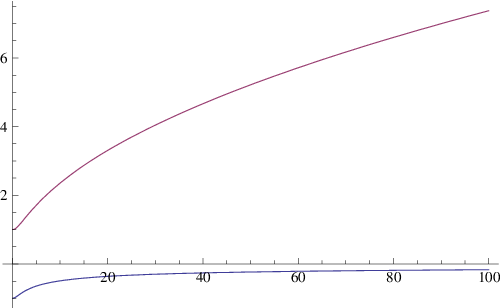
Refer to caption
Figure 1: A plot of the numerical behaviour of θ1L,d\theta_{1}^{L,d} and θ2L,u\theta_{2}^{L,u} for the coupled left-handed zero mode, shown for M=−1/2M=-1/2. The growing (but normalisable) mode is θ1L,d\theta_{1}^{L,d} and the decaying mode θ2L,u\theta_{2}^{L,u}.

6 Conclusions

Local brane realisations of the Standard Model around a (resolved) singularity have various phenomenologically attractive properties. They also drastically reduce the geometric complexity associated with global models. Furthermore, such local Standard Model constructions are forced on us by certain moduli stabilisation scenarios, such as the LARGE volume models of [16, 17].

In this paper we have studied certain aspects of such local D7 brane models in great detail. The paper has been devoted to studying the precise form of the wavefunctions that arise, through solving the appropriate differential equation for the zero modes. Compared to algebro-geometric approaches, the advantage of having explicit wavefunctions is that these are not restricted to holomorphic information and also contains information about the Kähler metric - the overlap of the wavefunctions directly gives the physical Yukawa couplings rather than simply the holomorphic component. The methods of this paper can be seen as an extension of the approach of [19] to local D7 brane models. Our particular emphasis has been the cases of branes wrapped on ℙ1×ℙ1\mathbb{P}^{1}\times\mathbb{P}^{1} and ℙ2\mathbb{P}^{2}, as these spaces represent the simplest examples where we can solve the Dirac and associated equations. We have dimensionally reduced super Yang-Mills on these surfaces, and solved the (twisted) equations to obtain the normalised zero modes for bifudamental fields that transform as scalars, spinors and vectors on the internal space. We have worked with both supersymmetric and non-supersymmetric brane configurations, and with Abelian and non-Abelian magnetic flux backgrounds. In ℙ2\mathbb{P}^{2} even though the Yukawa couplings vanish for both supersymmetric and non-supersymmetric Abelian flux, non-Abelian fluxes can lead to non-vanishing Yukawa couplings.

The cycle geometries have isometries which manifest themselves as flavour symmetries of the low-energy theory, acting on the zero modes. Where comparison is possible the zero mode degeneracies agree with those computed using index formulae. The Yukawa couplings vanish if we require a vanishing FI term, J∧F=0J\wedge F=0. If we allow J∧F≠0J\wedge F\neq 0, and assume either that the D-terms are cancelled by quantum corrections or field vevs or that the brane configuration is non-supersymmetric, then the Yukawa couplings can be non-vanishing.

Let us close by outlining some directions for future work.

  1. 1.

    We would like to extend this work to realistic D-brane models, where the gauge group resembles that of the MSSM. This will also require the construction of globally consistent brane configurations. This paper has focussed on obtaining the normalised wavefunctions and we have not imposed tadpole cancellation conditions. This is less important here where our focus is simply on the form of the wavefunctions, but for a complete and realistic model it will be necessary to ensure that the full brane configuration is consistent.

  2. 2.

    It would be instructive to understand the connection between the geometric Yukawa couplings and the Yukawa couplings in the singular limit, along the lines of [35]. In the singular limit anti-branes are supersymmetric objects and the Yukawa couplings can be non-vanishing for supersymmetric brane configurations. In the geometric limit the Yukawa couplings automatically vanish for supersymmetric brane configurations. It would be nice to understand better the interpolation between these two regimes.

  3. 3.

    It would be interesting to generalise the computations in this paper to more complex surfaces, such as del Pezzos. In some cases analytic metrics exist (e.g. see [36]) and it may be possible to explicitly solve the Dirac equation and compute the zero mode wavefunctions.

  4. 4.

    The techniques developed here may be extended to the case of Euclidean D3-branes wrapping the corresponding 4-cycle. This could be interesting to study instanton induced effective couplings in the four-dimensional effective action (see [37] for a recent review on these techniques).

  5. 5.

    The 4-surface metrics, for example the use of the Fubini-Study metric for ℙ2\mathbb{P}^{2}, are those appropriate for the case that the surface is embedded in a non-compact Calabi-Yau. In this case the local metric contains isometries that act as flavour symmetries of the Dirac equation. It would be interesting to obtain the form of the wavefunctions for surfaces embedded in Calabi-Yaus that are compact but of very large volume. In this case the largeness of the bulk provides a small breaking parameter for the local flavour symmetry [28]. By obtaining the wavefunctions on such perturbed spaces, possibly using numerical methods such as [38, 39, 40, 41], it will be possible to study explicitly the small breaking of flavour symmetry.

Acknowledgments.
For advice, encouragement and information we would like to thank Chris Beasley, Michele Cicoli, Diego Correa, Brian Dolan, Matt Dolan, Nick Dorey, Gary Gibbons, Sven Krippendorf, Harvey Reall, James Sparks, David Tong and Toby Wiseman. JC is funded by Trinity College, Cambridge and would like to thank the University of Texas at Austin for hospitality while part of this work was carried out. This work was supported in part by the National Science Foundation under NSF Grant PHY-0455649. AM is funded by STFC. Part of this work was carried out during his participation in the Tata Monsoon workshop of the International Center for Theoretical Studies of TIFR, he thanks the organizers for hospitality and support. FQ is funded by STFC and a Royal Society Wolfson Merit Award. He thanks the Mitchell family and the organizers of the Cook Branch’s meeting 2008 for hospitality.

Appendix A Kaluza-Klein vector modes

In this appendix we briefly note that scalar eigenfunctions of the Laplace equation automatically generate vector eigenfunctions, allowing the spectrum and profiles of KK vector modes to be derived from those of scalar vector modes. We use here the notation of section 2.

To do so we suppose that Φj,a​b=Xj​k​D~k​Ωa​b\Phi^{j,ab}=X^{jk}\tilde{D}_{k}\Omega^{ab}, where Ωa​b\Omega^{ab} is some scalar mode, and Xj​kX^{jk} is a covariantly constant tensor. In particular Xj​kX^{jk} may be either Jj​kJ^{jk} or gj​kg^{jk}, where Jj​kJ_{jk} is the almost complex structure. D~k=∇k−i​⟨A⟩ka​b\tilde{D}_{k}=\nabla_{k}-i\langle A\rangle_{k}^{ab} is the gauge covariant derivative acting on scalars. Then

D~i​D~i​Φj,a​b\displaystyle\tilde{D}_{i}\tilde{D}^{i}\Phi^{j,ab} =\displaystyle= D~i​D~i​Xj​k​D~k​Ωa​b\displaystyle\tilde{D}_{i}\tilde{D}^{i}X^{jk}\tilde{D}_{k}\Omega^{ab} (290)
=\displaystyle= D~i​(Xj​k​[D~i,D~k]+Xj​k​D~k​D~i)​Ωa​b.\displaystyle\tilde{D}_{i}\left(X^{jk}[\tilde{D}^{i},\tilde{D}_{k}]+X^{jk}\tilde{D}_{k}\tilde{D}^{i}\right)\Omega^{ab}.

Acting on a scalar, [D~i,D~k]​Ωa​b=−i​⟨G⟩i​ka​b​Ωa​b[\tilde{D}_{i},\tilde{D}_{k}]\,\Omega^{ab}=-i\langle G\rangle_{ik}^{ab}\,\Omega^{ab}, and so we obtain

D~i​D~i​Φj,a​b=D~i​(−i​Xj​k​⟨G⟩ki,a​b​Ωa​b)+D~i​(Xj​k​D~k​D~i)​Ωa​b.\tilde{D}_{i}\tilde{D}^{i}\Phi^{j,ab}=\tilde{D}_{i}\left(-iX^{jk}\langle G\rangle^{i\phantom{k},ab}_{\phantom{i}k}\Omega^{ab}\right)+\tilde{D}_{i}(X^{jk}\tilde{D}_{k}\tilde{D}^{i})\Omega^{ab}. (291)

Now, the flux is such that ⟨G⟩i​j∼ϵi​j\langle G\rangle_{ij}\sim\epsilon_{ij} and so is covariantly constant under ∇\nabla. Therefore,

D~i​⟨G⟩i​ka​b=⟨G⟩i​ka​b​D~i.\tilde{D}_{i}\langle G\rangle_{ik}^{ab}=\langle G\rangle_{ik}^{ab}\tilde{D}_{i}.

We then obtain

D~i​D~i​Φj,a​b\displaystyle\tilde{D}_{i}\tilde{D}^{i}\Phi^{j,ab} =\displaystyle= −i​Xj​k​⟨G⟩ki​a​b​D~i​Ωa​b+Xj​k​D~i​D~k​D~i​Ωa​b\displaystyle-iX^{jk}\langle G\rangle^{i\phantom{k}ab}_{\phantom{i}k}\tilde{D}_{i}\Omega^{ab}+X^{jk}\tilde{D}_{i}\tilde{D}_{k}\tilde{D}^{i}\Omega^{ab} (292)
=\displaystyle= −i​Xj​k​⟨G⟩ki​a​b​D~i​Ωa​b+Xj​k​[D~i,D~k]​(D~i​Ωa​b)+Xj​k​D~k​(D~i​D~i​Ωa​b).\displaystyle-iX^{jk}\langle G\rangle^{i\phantom{k}ab}_{\phantom{i}k}\tilde{D}_{i}\Omega^{ab}+X^{jk}[\tilde{D}_{i},\tilde{D}_{k}](\tilde{D}^{i}\Omega^{ab})+X^{jk}\tilde{D}_{k}(\tilde{D}_{i}\tilde{D}^{i}\Omega^{ab}).

Now as before [D~i,D~k][\tilde{D}_{i},\tilde{D}_{k}] on a vector gives [∇i,∇k]−i​⟨G⟩i​ka​b[\nabla_{i},\nabla_{k}]-i\langle G\rangle_{ik}^{ab}, and so we get

−12​g2​D~i​Φjb​a​D~i​Φj,a​b\displaystyle-\frac{1}{2g^{2}}\tilde{D}_{i}\Phi_{j}^{ba}\tilde{D}^{i}\Phi^{j,ab} =\displaystyle= Φjb​a2​g2​(−2​i​Xj​k​⟨G⟩i​k​D~i​Ωa​b+CLOSE\displaystyle\frac{\Phi_{j}^{ba}}{2g^{2}}\left(-2iX^{jk}\langle G\rangle_{ik}\tilde{D}^{i}\Omega^{ab}+\right. (293)
OPENXj​k​[∇i,∇k]​(D~i​Ωa​b)+Xj​k​D~k​(D~i​D~i​Ωa​b)).\displaystyle\left.X^{jk}[\nabla_{i},\nabla_{k}]\left(\tilde{D}^{i}\Omega^{ab}\right)+X^{jk}\tilde{D}_{k}\left(\tilde{D}_{i}\tilde{D}^{i}\Omega^{ab}\right)\right).

Φjb​a=Xjk​D~k​Ωb​a\Phi_{j}^{ba}=X_{j}^{k}\tilde{D}_{k}\Omega^{ba}, giving99 9 We supress the a​bab indices in ⟨G⟩\langle G\rangle to simplify the notation.

−12​g2​D~i​Φjb​a​D~i​Φj,a​b\displaystyle-\frac{1}{2g^{2}}\tilde{D}_{i}\Phi_{j}^{ba}\tilde{D}^{i}\Phi^{j,ab} =\displaystyle= D~p​Ωb​a2​g2​(−2​i​Xjp​Xj​k​⟨G⟩i​k​D~i​Ωa​b)\displaystyle\frac{\tilde{D}_{p}\Omega^{ba}}{2g^{2}}\left(-2iX_{j}^{p}X^{jk}\langle G\rangle_{ik}\tilde{D}^{i}\Omega^{ab}\right) (294)
+D~p​Ωb​a2​g2​Xjp​Xj​k​[∇i,∇k]​(D~i​Ωa​b)+D~p​Ωb​a2​g2​Xjp​Xj​k​D~k​(D~i​D~i​Ωa​b).\displaystyle+\frac{\tilde{D}_{p}\Omega^{ba}}{2g^{2}}X_{j}^{p}X^{jk}[\nabla_{i},\nabla_{k}]\left(\tilde{D}^{i}\Omega^{ab}\right)+\frac{\tilde{D}_{p}\Omega^{ba}}{2g^{2}}X_{j}^{p}X^{jk}\tilde{D}_{k}\left(\tilde{D}_{i}\tilde{D}^{i}\Omega^{ab}\right).

We now take Xj​k=gj​kX_{jk}=g_{jk}, and so Xjp​Xj​k=gp​kX_{j}^{p}X^{jk}=g^{pk}. In this case

−12​g2​D~i​Φjb​a​D~i​Φj,a​b\displaystyle-\frac{1}{2g^{2}}\tilde{D}_{i}\Phi_{j}^{ba}\tilde{D}^{i}\Phi^{j,ab} =\displaystyle= 12​g2[(D~pΩ)b​a(−2i⟨G⟩ip)D~iΩa​b+\displaystyle\frac{1}{2g^{2}}[(\tilde{D}_{p}\Omega)^{ba}(-2i\langle G\rangle_{i}^{p})\tilde{D}^{i}\Omega^{ab}+ (295)
(D~kΩ)b​a[∇i,∇k](D~iΩa​b)+(D~kΩb​a)D~k(D~lD~lΩa​b)]\displaystyle(\tilde{D}_{k}\Omega)^{ba}[\nabla_{i},\nabla_{k}](\tilde{D}^{i}\Omega^{ab})+(\tilde{D}^{k}\Omega^{ba})\tilde{D}_{k}(\tilde{D}_{l}\tilde{D}^{l}\Omega^{ab})]
=\displaystyle= 12​g2[(Φp)b​a(−2i⟨G⟩ip)Φia​b+\displaystyle\frac{1}{2g^{2}}[(\Phi_{p})^{ba}(-2i\langle G\rangle_{i}^{p})\Phi_{i}^{ab}+
(Φk)b​a[∇i,∇k](Φa​b)+(Φk,b​a)D~k(D~lD~lΩa​b)]\displaystyle(\Phi_{k})^{ba}[\nabla_{i},\nabla_{k}](\Phi^{ab})+(\Phi^{k,ba})\tilde{D}_{k}(\tilde{D}_{l}\tilde{D}^{l}\Omega^{ab})] (296)

Combining (296) with (56) we obtain a total result of

12​g2​(Dk​Ωb​a)​D~k​(D~l​D~l​Ωa​b)=−m22​g2​(Dk​Ωb​a)​(Dk​Ωa​b).\frac{1}{2g^{2}}(D^{k}\Omega^{ba})\tilde{D}_{k}\left(\tilde{D}_{l}\tilde{D}^{l}\Omega^{ab}\right)=-\frac{m^{2}}{2g^{2}}\left(D^{k}\Omega^{ba}\right)\left(D_{k}\Omega_{ab}\right).

In particular, all the flux and curvature contributions have cancelled, and if Ω\Omega is a scalar eigenfunction of D~i​D~i\tilde{D}_{i}\tilde{D}^{i} with eigenvalue −m2-m^{2}, then D~k​Ω\tilde{D}_{k}\Omega is also a vector eigenfunction with eigenvalue −m2-m^{2}.

A similar result is obtained for Xj​k=Jj​kX_{jk}=J_{jk}: the vector mode Φj,a​b=Xj​k​D~k​Ωa​b\Phi^{j,ab}=X^{jk}\tilde{D}_{k}\Omega^{ab} is a vector eigenfunction with mass −m2-m^{2}. On their own neither of these two modes satisfy the gauge-fixing condition D~i​Φi,a​b=0\tilde{D}_{i}\Phi^{i,ab}=0. However the gauge-fixing condition can be satisfied by writing

Φj,a​b=α​gj​k​D~k​Ωa​b+β​Jj​k​D~k​Ωa​b,\Phi^{j,ab}=\alpha\,g^{jk}\tilde{D}_{k}\Omega^{ab}+\beta\,J^{jk}\tilde{D}_{k}\Omega^{ab}, (297)

for appropriate constants α\alpha and β\beta.

Appendix B Patches

In this section we give some details as to the explicit patch transition functions for the fermionic wavefunctions on ℙ1\mathbb{P}^{1}. We start with coordinates z,z¯z,\bar{z} with

d​s2=4​d​z​d​z¯(1+z​z¯)2.ds^{2}=\frac{4dzd\bar{z}}{(1+z\bar{z})^{2}}. (298)

These coordinates are good for describing all of ℙ1\mathbb{P}^{1} except the point at ∞\infty. We denote this patch by 𝒜\mathcal{A}. To describe the point at infinity, we must change patches to the patch ℬ\mathcal{B} coordinatised by u=−1/zu=-1/z. The functional form of the metric is unaltered,

d​s2=4​d​u​d​u¯(1+u​u¯)2.ds^{2}=\frac{4dud\bar{u}}{(1+u\bar{u})^{2}}. (299)

Assoicated with the patches 𝒜\mathcal{A} and ℬ\mathcal{B} there are two separate vielbeins that are both valid in the overlap region 𝒜​∫ℬ\mathcal{A}\int\mathcal{B}, e𝒜1,e𝒜2e_{\mathcal{A}}^{1},e_{\mathcal{A}}^{2} and eℬ1,eℬ2e_{\mathcal{B}}^{1},e_{\mathcal{B}}^{2}. We have

e𝒜,z1=e𝒜,z¯1=11+z​z¯,\displaystyle e^{1}_{\mathcal{A},z}=e^{1}_{\mathcal{A},\bar{z}}=\frac{1}{1+z\bar{z}}, e𝒜,z2=−e𝒜,z¯2=i1+z​z¯.\displaystyle e^{2}_{\mathcal{A},z}=-e^{2}_{\mathcal{A},\bar{z}}=\frac{i}{1+z\bar{z}}.
eℬ,u1=eℬ,u¯1=11+u​u¯,\displaystyle e^{1}_{\mathcal{B},u}=e^{1}_{\mathcal{B},\bar{u}}=\frac{1}{1+u\bar{u}}, eℬ,u2=−eℬ,u¯2=i1+u​u¯.\displaystyle e^{2}_{\mathcal{B},u}=-e^{2}_{\mathcal{B},\bar{u}}=\frac{i}{1+u\bar{u}}. (300)

Using the coordinate relation u=−z−1u=-z^{-1} that holds on the overlap region, we find that the two vielbeins are related by

eℬ,zi=(z¯z)​e𝒜,zi,eℬ,z¯i=(zz¯)​e𝒜,z¯i.e^{i}_{\mathcal{B},z}=\left(\frac{\bar{z}}{z}\right)e^{i}_{\mathcal{A},z},\qquad e^{i}_{\mathcal{B},\bar{z}}=\left(\frac{z}{\bar{z}}\right)e^{i}_{\mathcal{A},\bar{z}}.

In terms of real vectors e1e^{1} and e2e^{2}, we can write

(eℬ1eℬ2)=(cos⁡(2​θ)−sin⁡(2​θ)sin⁡(2​θ)cos⁡(2​θ))​(e𝒜1e𝒜2).\left(\begin{array}[]{c}e^{1}_{\mathcal{B}}\\ e^{2}_{\mathcal{B}}\end{array}\right)=\left(\begin{array}[]{cc}\cos(2\theta)&-\sin(2\theta)\\ \sin(2\theta)&\cos(2\theta)\end{array}\right)\left(\begin{array}[]{c}e^{1}_{\mathcal{A}}\\ e^{2}_{\mathcal{A}}\end{array}\right). (301)

Lifting this to an action on spinors using Λ~=exp⁡(14​ωα​β​Λα​β)\tilde{\Lambda}=\exp\left(\frac{1}{4}\omega^{\alpha\beta}\Lambda_{\alpha\beta}\right), we obtain ψB=𝒪𝒜​ℬ,s​p​i​n​ψA\psi_{B}=\mathcal{O}_{\mathcal{AB},spin}\psi_{A}, with

𝒪𝒜​ℬ,s​p​i​n=((z¯z)1/200(zz¯)1/2).\mathcal{O}_{\mathcal{AB},spin}=\left(\begin{array}[]{cc}\left(\frac{\bar{z}}{z}\right)^{1/2}&0\\ 0&\left(\frac{z}{\bar{z}}\right)^{1/2}\end{array}\right). (302)

In the presence of a nonvanishing gauge background there is an additional gauge contribution to the transition functions. The gauge fields on the two patches are

A𝒜\displaystyle A_{\mathcal{A}} =\displaystyle= i​M​z¯​d​z2​(1+z​z¯)−i​M​z​d​z¯2​(1+z​z¯),\displaystyle\frac{iM\bar{z}dz}{2(1+z\bar{z})}-\frac{iMzd\bar{z}}{2(1+z\bar{z})},
Aℬ\displaystyle A_{\mathcal{B}} =\displaystyle= i​M​u¯​d​u2​(1+u​u¯)−i​M​u​d​u¯2​(1+u​u¯).\displaystyle\frac{iM\bar{u}du}{2(1+u\bar{u})}-\frac{iMud\bar{u}}{2(1+u\bar{u})}. (303)

We can verify that on the overlap region these are related by

Aℬ=A𝒜+d⁡(i​ln⁡(z¯z)M/2)≡A1+d​λ,A_{\mathcal{B}}=A_{\mathcal{A}}+d\left(i\ln\left(\frac{\bar{z}}{z}\right)^{M/2}\right)\equiv A_{1}+d\lambda, (304)

and so the gauge transition function is

𝒪𝒜​ℬ,g​a​u​g​e=ei​λ=e−ln⁡(z¯z)M/2=(zz¯)M/2.\mathcal{O}_{\mathcal{A}\mathcal{B},gauge}=e^{i\lambda}=e^{-\ln\left(\frac{\bar{z}}{z}\right)^{M/2}}=\left(\frac{z}{\bar{z}}\right)^{M/2}.

The overall patch transition function is then

𝒪𝒜​ℬ=𝒪𝒜​ℬ,s​p​i​n​𝒪𝒜​ℬ,g​a​u​g​e=((z¯z)1−M200(zz¯)1+M2).\mathcal{O}_{\mathcal{AB}}=\mathcal{O}_{\mathcal{AB},spin}\mathcal{O}_{\mathcal{AB},gauge}=\left(\begin{array}[]{cc}\left(\frac{\bar{z}}{z}\right)^{\frac{1-M}{2}}&0\\ 0&\left(\frac{z}{\bar{z}}\right)^{\frac{1+M}{2}}\end{array}\right). (305)

Acting on zero modes of the Dirac equation with the patch transition function, we obtain

𝒪𝒜​ℬ​(ψ1​(z,z¯)ψ2​(z,z¯))=𝒪𝒜​ℬ​(f𝒜​(z¯)​(1+z​z¯)(1−M2)g𝒜​(z)​(1+z​z¯)(1+M2))=(fℬ​(u¯)​(1+u​u¯)(1−M2)gℬ​(u)​(1+u​u¯)(1+M2)),\mathcal{O}_{\mathcal{AB}}\left(\begin{array}[]{c}\psi_{1}(z,\bar{z})\\ \psi_{2}(z,\bar{z})\end{array}\right)=\mathcal{O}_{\mathcal{AB}}\left(\begin{array}[]{c}f_{\mathcal{A}}(\bar{z})(1+z\bar{z})^{\left(\frac{1-M}{2}\right)}\\ g_{\mathcal{A}}({z})(1+z\bar{z})^{\left(\frac{1+M}{2}\right)}\end{array}\right)=\left(\begin{array}[]{c}f_{\mathcal{B}}(\bar{u})(1+u\bar{u})^{\left(\frac{1-M}{2}\right)}\\ g_{\mathcal{B}}({u})(1+u\bar{u})^{\left(\frac{1+M}{2}\right)}\end{array}\right), (306)

where both f𝒜,g𝒜f_{\mathcal{A}},g_{\mathcal{A}} and fℬ,gℬf_{\mathcal{B}},g_{\mathcal{B}} are analytic polynomials of maximal degree |M|−1|M|-1. The patch transition functions therefore indeed take normalised solutions of the Dirac equation to normalised solutions of the Dirac equation.

References

  • [1] R. Blumenhagen, M. Cvetic, P. Langacker and G. Shiu, Ann. Rev. Nucl. Part. Sci. 55, 71 (2005) [arXiv:hep-th/0502005].
  • [2] R. Blumenhagen, B. Kors, D. Lust and S. Stieberger, Phys. Rept. 445, 1 (2007) [arXiv:hep-th/0610327].
  • [3] F. Marchesano, Fortsch. Phys. 55 (2007) 491 [arXiv:hep-th/0702094].
  • [4] D. Malyshev and H. Verlinde, Nucl. Phys. Proc. Suppl. 171 (2007) 139 [arXiv:0711.2451 [hep-th]].
  • [5] H. P. Nilles, S. Ramos-Sanchez, M. Ratz and P. K. S. Vaudrevange, arXiv:0806.3905 [hep-th].
  • [6] G. Aldazabal, L. E. Ibanez, F. Quevedo and A. M. Uranga, JHEP 0008, 002 (2000) [arXiv:hep-th/0005067]; J. F. G. Cascales, M. P. Garcia del Moral, F. Quevedo and A. M. Uranga, JHEP 0402 (2004) 031 [arXiv:hep-th/0312051].
  • [7] L. F. Alday and G. Aldazabal, JHEP 0205, 022 (2002) [arXiv:hep-th/0203129].
  • [8] H. Verlinde and M. Wijnholt, JHEP 0701, 106 (2007) [arXiv:hep-th/0508089].
  • [9] J. Gray, Y. H. He, V. Jejjala and B. D. Nelson, Nucl. Phys. B 750 (2006) 1 [arXiv:hep-th/0604208].
  • [10] M. Buican, D. Malyshev, D. R. Morrison, H. Verlinde and M. Wijnholt, JHEP 0701, 107 (2007) [arXiv:hep-th/0610007].
  • [11] M. Wijnholt, arXiv:hep-th/0703047.
  • [12] C. Beasley, J. J. Heckman and C. Vafa, arXiv:0802.3391 [hep-th].
  • [13] L. Aparicio, D. G. Cerdeno and L. E. Ibanez, arXiv:0805.2943 [hep-ph].
  • [14] C. Beasley, J. J. Heckman and C. Vafa, arXiv:0806.0102 [hep-th].
  • [15] R. Tatar and T. Watari, arXiv:0806.0634 [hep-th].
  • [16] V. Balasubramanian, P. Berglund, J. P. Conlon and F. Quevedo, JHEP 0503, 007 (2005) [arXiv:hep-th/0502058].
  • [17] J. P. Conlon, F. Quevedo and K. Suruliz, JHEP 0508, 007 (2005) [arXiv:hep-th/0505076].
  • [18] J. P. Conlon and D. Cremades, Phys. Rev. Lett. 99, 041803 (2007) [arXiv:hep-ph/0611144].
  • [19] D. Cremades, L. E. Ibanez and F. Marchesano, JHEP 0405 (2004) 079 [arXiv:hep-th/0404229].
  • [20] H. Abe, T. Kobayashi and H. Ohki, arXiv:0806.4748 [hep-th].
  • [21] C. N. Pope, Phys. Lett. B 97, 417 (1980).
  • [22] D. Karabali and V. P. Nair, Nucl. Phys. B 641 (2002) 533 [arXiv:hep-th/0203264].
  • [23] B. P. Dolan and C. Nash, JHEP 0210 (2002) 041 [arXiv:hep-th/0207078].
  • [24] B. P. Dolan, JHEP 0305 (2003) 018 [arXiv:hep-th/0304037].
  • [25] R. P. Andrews and N. Dorey, Phys. Lett. B 631 (2005) 74 arXiv:hep-th/0505107.
  • [26] M. Bershadsky, C. Vafa and V. Sadov, Nucl. Phys. B 463 (1996) 420 [arXiv:hep-th/9511222].
  • [27] N. K. Nielsen and P. Olesen, Nucl. Phys. B 144, 376 (1978).
  • [28] C. P. Burgess, J. P. Conlon, L. Y. Hung, C. H. Kom, A. Maharana and F. Quevedo, arXiv:0805.4037 [hep-th].
  • [29] D. Z. Freedman and G. W. Gibbons, “New Higher Dimensional Ricci Flat Kahler Metrics,”, ITP Preprint ITP-SB-80-48 (unpublished).
  • [30] C. A. Lutken, J. Phys. A 21 (1988) 1889.
  • [31] S. W. Hawking and C. N. Pope, Phys. Lett. B 73 (1978) 42.
  • [32] D. S. Freed and E. Witten, arXiv:hep-th/9907189.
  • [33] J. M. Charap and M. J. Duff, Phys. Lett. B 69, 445 (1977).
  • [34] G. W. Gibbons and C. N. Pope, Commun. Math. Phys. 61, 239 (1978).
  • [35] S. G. Nibbelink, D. Klevers, F. Ploger, M. Trapletti and P. K. S. Vaudrevange, JHEP 0804 (2008) 060 [arXiv:0802.2809 [hep-th]].
  • [36] T. Oota and Y. Yasui, Phys. Lett. B 639, 54 (2006) [arXiv:hep-th/0605129].
  • [37] N. Akerblom, R. Blumenhagen, D. Lust and M. Schmidt-Sommerfeld, arXiv:0712.1793 [hep-th].
  • [38] M. Headrick and T. Wiseman, Class. Quant. Grav. 22 (2005) 4931 [arXiv:hep-th/0506129].
  • [39] M. R. Douglas, R. L. Karp, S. Lukic and R. Reinbacher, J. Math. Phys. 49 (2008) 032302 [arXiv:hep-th/0612075].
  • [40] C. Doran, M. Headrick, C. P. Herzog, J. Kantor and T. Wiseman, arXiv:hep-th/0703057.
  • [41] V. Braun, T. Brelidze, M. R. Douglas and B. A. Ovrut, JHEP 0805, 080 (2008) [arXiv:0712.3563 [hep-th]].