New aspects of leptogenesis bounds
Abstract
We present a general analysis that reveals new aspects of the leptogenesis bounds on neutrino masses and on the reheat temperature of the Universe. After revisiting a known effect coming from an unbounded term in the total asymmetry, we show that an unbounded term in the flavored asymmetries has a stronger impact. It relaxes the lower bound on the reheat temperature down to for and for a mild tuning of the parameters in the see-saw orthogonal matrix. We also consider the effect of the Higgs asymmetry, showing that it lowers the upper bound on the neutrino masses in the so-called fully flavored regime where classic Boltzmann equations can be used. Imposing independence of the initial conditions contributes to lower the upper bound on neutrino masses as well. We study the conditions for the validity of the usual -dominated scenario and for the applicability of the lower bound on the lightest right-handed (RH) neutrino mass . We find that except for the two effective RH neutrino scenario, recovered for , and for values , the final asymmetry is more naturally dominated by the contribution from -decays. Finally, we confirm in a general way that going beyond the hierarchical limit, the effect of washout addition makes the lower bound on more stringent for .
1 Introduction
Leptogenesis [1] provides an elegant solution to the problem of the non-observation of primordial antimatter in the Universe. An appealing feature of this mechanism is that it relies on a minimal extension of the Standard Model (SM) where RH neutrinos are added to the Lagrangian. In the see-saw limit [2], small neutrino masses can be naturally accommodated in agreement with the data. Considering, for definiteness, the simplest and best motivated case of three additional RH neutrinos, only few of the eighteen new parameters, three neutrino masses, three mixing angles and three CP violating phases, are or can hopefully be probed in neutrino experiments. The remaining 9 ‘high-energy’ parameters are out of reach in low energy experiments. In this respect, leptogenesis represents also an important cosmological tool to access information on this ‘dark side’ of the see-saw parameter space.
In an unflavored analysis and in a traditional -dominated scenario, where it is assumed that the final asymmetry is dominantly produced from the lightest RH neutrino decays, one finds a lower bound on the lightest RH neutrino mass [3, 4]. This is given by [5, 6] at the onset of the strong washout regime, where the final asymmetry does not depend on the initial conditions. This lower bound also implies an associated lower bound on the reheat temperature, [7, 8, 6]. In addition an upper bound on the neutrino masses, , holds as well [9].
A mild hierarchy in the spectrum of the RH neutrino masses, such that , is a necessary condition for the validity of the -dominated scenario but is not sufficient. Indeed, upon closer inspection, the observed asymmetry can still be generated from the decays of the next-to-lightest RH neutrinos, realizing a -dominated scenario [5]. The lower bound on is replaced by a lower bound on but this still implies a lower bound on . It is therefore more correct to say that leptogenesis yields a lower bound on rather than on .
Even when flavor effects are considered [10, 11] (see also [12, 13]), the lower bound on has been found not to change [6]. On the other hand they induce other important modifications. First, the final asymmetry receives an additional contribution that also depends on neutrino mixing parameters [10, 14] and an interesting feature is that such an additional contribution can originate solely by low-energy (Dirac or Majorana) phases [10] and can even explain the whole observed asymmetry [6, 15, 16, 17, 18, 19]. Second, flavor effects can relax the stringent upper bound on the neutrino masses, , holding in the unflavored regime when a hierarchical heavy neutrino mass spectrum is assumed [9]. In [11], it was found that flavor effects completely erase this upper bound. However, in [20], it was pointed out that this conclusion relies on the use of classical Boltzmann equations beyond their range of validity and has therefore to be checked within a more general description making use of density matrix equations. In [21] it was found that using classic Boltzmann equations neutrino masses as large as are possible, a value larger than the upper bound holding in the unflavored regime and than the current upper bound from cosmological observations. A similar conclusion has been recently obtained in [22] as well.
Many of these results have been obtained employing different assumptions or restrictions in the parameter space. In this paper we revisit in detail the leptogenesis bounds still assuming classical Boltzmann equations and the -dominated scenario but without further restrictions on the parameter space and relaxing many assumptions that are usually made. For example, we find more general conditions for the validity of the -dominated scenario. In general, our analysis reveals various new aspects including effects confirming the necessity to go beyond a classical Boltzmann kinetic approach to solve the problem of the upper bound on the neutrino masses.
In Section 2 we set up the general notation. In Section 3 we show that the final asymmetry can be written as the sum of different contributions acting independently of each other. The first step is to distinguish between a contribution from the lightest RH neutrino decays and a contribution from the heavier RH neutrino decays, just two in our case. In a traditional -dominated scenario the first one is dominant. This can be still conveniently re-cast as the sum of an unflavored term plus a flavored term. Finally, the unflavored term can be further decomposed into a piece proportional to a contribution to the total asymmetry respecting the usual upper bound [23, 3] and into a term that is not upper bounded but vanishes when . If , this term is typically strongly suppressed when a mild hierarchy is assumed and barring a fine-tuned choice of the parameters [24, 25, 5]. Analogously, we recast also the flavored asymmetries as the sum of an upper-bounded term plus an unbounded extra-term that has been neglected in previous works but that proves to be important in interesting cases.
In the end of Section 3 we review, as a starting point for our analysis, the neutrino mass bounds that arise in the minimal scenario, that we call ‘vanilla leptogenesis’, when all simplifications are made at once: the heavier RH neutrino contribution, the flavored terms and the extra-term to the total asymmetry are neglected and the hierarchical limit is taken. In this case the final asymmetry depends only on 6 parameters [7, 5].
In Section 4 we show the role played by the unbounded term in the total asymmetry of the lightest RH neutrino, , that has to be considered when [24, 25, 5]. We study its effect on the bounds in a quite conservative mild hierarchical limit , showing how a rotation in the complex 2-3 plane is the most effective ingredient in enhancing this term and showing that the bounds get modified only for fine tuned parameter choices. Our analysis shows moreover that this extra-term acts independently of flavor effects.
In Section 5 we study how the bounds change when flavor effects are taken into account and, interestingly, we show that a so far neglected term in the flavored asymmetries is actually able to relax the lower bound on the reheating temperature in presence of wash-out. In the case of the upper bound on the absolute neutrino mass scale, we show that this is sensitive to a variation of different assumptions and conditions. We also show that, taking into account the Higgs asymmetry then, within the validity of classical Boltzmann equations, one cannot say whether the bound holding in the unflavored regime is evaded. This conclusion is strengthened when independence of the initial conditions is imposed.
In Section 6 we consider the contribution from the two heavier RH neutrinos, including flavor effects and still assuming the hierarchical limit, showing a (non-trivial) sufficient condition for the -dominated scenario to hold.
Finally, in Section 7, we show how the neutrino mass bounds change going beyond the limit of hierarchical RH neutrinos when flavor effects are included. Contrarily to a naive expectation, we show that the allowed region, instead of getting enlarged, actually shrinks when mild degeneracies for the heavy neutrinos masses are considered. The bounds get relaxed only when the heavy neutrino mass degeneracies are much smaller than those of the light neutrinos.
2 General set-up
Leptogenesis is based on a popular extension of the Standard Model,
| (1) |
where three RH neutrinos , with a Majorana mass term and Yukawa couplings , are added. After spontaneous symmetry breaking, a Dirac mass term , is generated by the vev GeV of the Higgs boson. In the see-saw limit, , the spectrum of neutrino mass eigenstates splits in two sets: 3 very heavy neutrinos, and respectively with masses almost coinciding with the eigenvalues of , and 3 light neutrinos with masses , the eigenvalues of the light neutrino mass matrix given by the see-saw formula [2],
| (2) |
Neutrino oscillation experiments measure two neutrino mass-squared differences. For normal schemes one has and , whereas for inverted schemes one has and . For [26] the spectrum is quasi-degenerate, while for [26] it is fully hierarchical (normal or inverted). The most stringent upper bound on the absolute neutrino mass scale comes from cosmological observations. Recently, quite a conservative upper bound,
| (3) |
has been obtained by the WMAP collaboration combining CMB, baryon acoustic oscillations and supernovae type Ia observations [27].
With leptogenesis, this simple extension of the Standard Model is also able to explain the observed baryon asymmetry of the Universe [27]
| (4) |
It is widely known that, in order to generate a baryon asymmetry in the early Universe, one needs to satisfy the three Sakharov conditions [28]. At temperatures , baryon number is violated by the non-perturbative sphaleron processes [29]. Moreover is violated in the decays of the heavy RH neutrinos. Indeed the Dirac mass matrix is in general complex and this provides a natural source of violation. At the same time departure from thermal equilibrium occurs in the decays of the heavy RH neutrinos as well. This can be conveniently quantified in terms of the decay parameters, defined as , given by the ratio of the decay widths to the expansion rate when the RH neutrinos become non-relativistic. The decay parameters can be expressed in terms of the Yukawa couplings by
| (5) |
are the effective neutrino masses and is the equilibrium neutrino mass [7] given by
| (6) |
There are two ways how violation can manifest itself. A first one is given by having a decay rate of into leptons, , different from the decay rate into anti-leptons, . This is parameterized by the total asymmetries
| (7) |
A perturbative calculation from the interference of tree level with one loop self-energy and vertex diagrams gives [30]
| (8) |
having introduced [9]
| (9) |
A second way [10] is given by the possibility that in general, indicating with the final lepton quantum state and with the final anti-lepton quantum state, one has . This can be easily understood when the flavor composition of the final lepton state is considered. Indeed, introducing the projectors on the flavor eigenstates, they can be written like the sum of two terms,
| (10) | |||||
| (11) |
The first term is the tree level contribution and is common to both projectors but the second term, from loop corrections, changes sign and gives rise to a different flavor composition when . These two violating effects translate respectively in two separate terms in the flavored asymmetries,
| (12) |
where and . The flavored asymmetries can be calculated using [30]
| (13) |
The second violating contribution yields an additional contribution to the final asymmetry only if the flavor composition plays a role in the determination of the final asymmetry. This depends on the effectiveness of the charged lepton interactions implied by the term in the Lagrangian, which is diagonal in flavor space. The latter implies that the processes and and the CP conjugated, (where are the gauge bosons) occur at a rate [31]. If these processes are effective, then they measure the flavor composition of the final leptons and this becomes a relevant ingredient in the determination of the final asymmetry if a second condition is fulfilled as well, as we will comment.
In the hierarchical limit the decays of just one species of RH neutrino, the lightest [1] or the next-to-lightest [5], dominantly contribute to the final asymmetry. If during the relevant period of the asymmetry generation, where denotes the inverse-decay rate, then the coherence of the lepton states is preserved on average between a decay and a subsequent inverse decays and the unflavored regime, where flavor effects are negligible, holds. This requirement implies [20]
| (14) |
In this case an approximate set of Boltzmann equations is given by
| (15) | |||||
| (16) |
where and where we indicated with any particle number or asymmetry calculated in a portion of co-moving volume containing one heavy neutrino in ultra-relativistic thermal equilibrium, so that . With this convention, the predicted baryon-to-photon ratio is related to the final value of the final asymmetry by the relation
| (17) |
where , and . Defining and , the decay factors are given by
| (18) |
where is the expansion rate. The total decay rates, , are the product of the decay widths times the thermally averaged dilation factors , given by the ratio of the modified Bessel functions. The equilibrium abundance and its rate are also expressed through the modified Bessel functions,
| (19) |
After proper subtraction of the resonant contribution from processes [32], the inverse decay washout terms are simply given by
| (20) |
The washout term is the non-resonant processes contribution. It gives a non-negligible effect only at and in this case it can be approximated as [7]
| (21) |
where and . Notice that we are neglecting scatterings [33, 14], giving a correction to a level less than [6], thermal corrections [8], giving relevant (though with big theoretical uncertainties) corrections only in the weak washout, and spectator processes [34, 35], that produce corrections to a level less than [35].
On the other hand, if the charged lepton Yukawa interactions are in equilibrium () and faster than inverse decays, i.e.
| (22) |
during the relevant period of the asymmetry generation, then lepton quantum states lose coherence between the production at decay and the subsequent absorption in inverse processes. If the quantum state becomes completely incoherent and is fully projected on one of the flavor eigenstates, each lepton flavor eigenstate can be treated as a statistically independent particle species and a ‘fully flavored regime’ is obtained. Note that one has to distinguish a two-flavor regime, for , such that the condition Eq. (22) is satisfied only for , and a three-flavor regime, where it applies also to .
In the fully flavored regime (two or three flavors), classical Boltzmann equations can be still used like in the unflavored regime, with the difference, in general, that now each single flavor asymmetry has to be tracked independently. Since sphaleron processes conserve the quantities (), these are the convenient independent variables to be used in the set of Boltzmann equations that can be written as
| (23) | |||||
| (24) |
where we are using the same approximations as in the unflavored case but neglecting the non-resonant term, since this counts only for like also a contribution from processes that one has to consider in the flavored case. Notice that the final asymmetry is now calculated as .
The matrix [12] relates the asymmetries stored in lepton doublets, , to the asymmetries asymmetries and is given, in a two-flavor regime, by [14]
| (25) |
The matrix takes into account the washout due to the asymmetry stored in the Higgs field [10] and is given by
| (26) |
The Higgs asymmetry has been neglected so far but, as we will see, it has a relevant effect on the upper bound on the neutrino masses. Indeed the sum of the two matrices gives
| (27) |
The off-diagonal terms give a small effect in the calculation of the final asymmetry [14] and therefore, in the end, one can safely use the approximation in the derivation of the bounds. In Section 5 we will compare the results when the Higgs asymmetry is neglected, when it is taken into account and when one uses the approximation , showing that the latter works very well justifying its use for the remainder of the paper.
Taking for simplicity the two flavor case, it is instructive to sum over the flavor Eq. (24), obtaining
| (28) |
This equation clearly shows that when the washout vanishes there must be no difference between the unflavored and the fully flavored regime. Therefore, the lower bounds on and on obtained in the limit of no-washout, rigorously for an initial thermal abundance and approximately for an initial vanishing abundance, do not change when flavor effects are taken into account [6].
A convenient parametrization of the Dirac mass matrix is obtained in terms of the orthogonal matrix [36]
| (29) |
where we defined and . The matrix diagonalizes the light neutrino mass matrix , such that , and it can be identified with the lepton mixing matrix in a basis where the charged lepton mass matrix is diagonal. We will adopt the parametrization [37]
| (30) |
where , and, neglecting the statistical errors, we will use and , compatible with the results from neutrino oscillation experiments. Moreover, we will adopt the range , allowed from a global analysis for unitary [26], an approximation that holds with great precision in the see-saw limit with . With the adopted convention for the light neutrino masses, , this parametrization is valid only for normal hierarchy, while for inverted hierarchy one has to perform a column cyclic permutation. In a general analysis, leptogenesis bounds are not depending on the scheme, normal or inverted, but in restricted scenarios, like in the effective two RH neutrino scenario where the third is very heavy and decouples or in ‘Dirac phase leptogenesis’ [19], differences can arise and depend on flavor effects. We will signal these differences in our analysis.
It will also prove useful to introduce the following parametrization for the see-saw orthogonal matrix in terms of complex rotations
| (31) |
where
| (32) |
and where the overall sign takes into account the possibility of a parity transformation as well. Notice that, using the orthogonal parametrization, Eq. (29), the effective neutrino masses, and consequently the decay parameters, can be expressed as linear combinations of the neutrino masses [38, 7], such that . Notice that the orthogonality of is equivalent to the see-saw relation for the light neutrino masses and in particular one has that is the contribution to from the term . Therefore, large absolute values of the entries imply a strong fine tuning not only because they require phase cancelations but also because they imply that neutrino masses are much lighter than terms because of sign cancelations. Therefore, such choices tend to transfer the explanation of neutrino lightness from the see-saw mechanism to some other mechanism that has to explain the fine-tuned cancelations. The interest for considering models with very large is merely phenomenological since they make possible to satisfy neutrino masses with the see-saw mechanism and at the same time to have RH neutrinos with large Yukawa’s, making possible to detect them in colliders [39]. This will not be our point of view in this paper and we will conventionally consider orthogonal matrices to be ‘reasonable’ if , implying , and ‘acceptable’ if , implying . These will be the two benchmark cases that we will adopt in the plots.
3 Vanilla leptogenesis
Using the approximation , a general solution for the final asymmetry can be written as [6]
| (34) |
with the final values of the 9 efficiency factors given by
| (35) |
This solution holds both in the fully flavored regime and in the unflavored regime, adopting the convention that when the condition (14) applies, all projectors . It is indeed easy to verify that in this case, summing over the flavor, the set of equations (24) reduces to Eq. (16). On the other hand it should be also noticed that Eq. (24) holds only if the condition (22) is respected and this, when applied to the decays and inverse decays, translates into
| (36) |
For there is an intermediate regime where the unflavored regime does not hold but at the same time the validity of the Eq. (24), and therefore of the expression (34), is not guaranteed. We will signal in the plots the results obtained in the fully flavored regime but for which the condition (36) is not satisfied. These results should be therefore checked within a more general kinetic description employing density matrix equations able to describe the regime where coherence (or decoherence) of the final lepton quantum state is only partial.
Notice that the ’s are the values of possible pre-existing flavored asymmetries. In the unflavored regime is the only parameter that determines whether the final asymmetry depends or not on a possible pre-existing asymmetry [9]. Taking into account flavor effects the problem is more involved and there are different issues to be considered. Here we will not face this problem and we will simply assume that the first term is negligible.
It is instructive to re-cast the Eq. (34) in an approximate way that enlightens different effects and contributions. For definiteness, we consider the two-flavor regime holding for . The total asymmetry can be recast as [5]
| (37) |
where, defining
| (38) |
one has
| (39) |
and
| (40) |
With these definitions, the final asymmetry can be written approximately as
| (41) | |||||
where is an effective number of flavors. In the unflavored regime one has , and in the fully flavored regime, if both flavors experience a strong washout (), one has approximately , while in general .
The simplest scenario, that we call vanilla leptogenesis borrowing the name from observational cosmology, corresponds to taking all possible simplifying assumptions:
- 1.
hierarchical limit, , so that ;
- 2.
negligible contribution from the heavier RH neutrinos;
- 3.
negligible flavor effects ( and );
- 4.
, so that .
The calculation of the final asymmetry then simply reduces to
| (42) |
depending only on 6 unknown parameters. The efficiency factor is well approximated by [7]
| (43) |
For the case of a thermal initial -abundance (), one has
| (44) |
where is approximately given by the expression [43]
| (45) |
In the relevant range this expression is further well approximated by the simple power-law [44].
In the case of a vanishing initial -abundance (), one has to take into account both a negative and a positive contribution, such that
| (46) |
The analytic expressions for and can be found in [7]. Imposing that the predicted final asymmetry, Eq. (17), explains the observed one, Eq. (4), yields the condition
| (47) |
where we defined
| (48) |
The last inequality gives the value of that we used in the plots to obtain the allowed region in the plane scanning over all values of and . The result is shown in the central panel of Fig. 1.


One can notice the presence of the usual lower bound on the lightest RH neutrino mass, for initial vanishing abundance and for initial thermal abundance [4]. This can be easily inferred from the Eq. (47) neglecting the exponential factor in Eq. (43) and using the well-known upper bound
| (49) |
where the function is unity in the limit , and vanishes for . This function can be derived analytically together with simple analytic expressions valid in particular regimes [5]. For and for initial thermal abundance one simply finds , in agreement with the numerical result. From the central panel of Fig. 1 one can also notice that vanilla letogenesis predicts [9], in agreement with the current observational upper bound (cf. Eq. (3)). In the plots the hatched region indicates the excluded values. This upper bound can be derived analytically as well [7].
We performed a simple exercise showing how the allowed region in the plane would have been for values of and different from the true measured ones. We kept the ratio constant. In the left panel , while in the right panel . One can see how the allowed region shrinks considerably, and almost disappears for these extreme values. This is one way to show the ‘leptogenesis conspiracy’ [45], that means how, order-of-magnitude-wise, the measured atmospheric and solar neutrino mass scales are optimal for leptogenesis to be successful. It should be noticed that for , even though the lower bound on is much lower, the density of points in the allowed region is very low since they correspond to a very fine-tuned situation where .


In Fig. 2 we show the bounds for particular choices of the orthogonal matrix: in the left panel for , corresponding to , and in the right panel for the effective two RH neutrino case obtained in the limit and corresponding to an orthogonal matrix with . In the first case, one can see how the bounds do not change compared to the general case, showing that this is the choice saturating the bounds, a well-known result [4]. Notice that for there is no dependence of the bounds on the light neutrino mass scheme, normal or inverted, and therefore, in vanilla leptogenesis, normal or inverted schemes produce the same bounds [4]. On the other hand, in the second case the lower bound on becomes more stringent [41], especially in the case of inverted hierarchy. Indeed, in the vanilla case, for the same choice of the orthogonal matrix, the final asymmetry in an inverted scheme can be only less than in a normal scheme, or at most equal in the special case , as discussed analytically in [5]. This result is easy to understand qualitatively: the dominant term in the asymmetry is suppressed when the neutrino masses increase, either when increases, or switching from normal to inverted hierarchy since in this case gets higher.
In the next sections we will relax the assumptions of vanilla leptogenesis, studying how the leptogenesis bounds change accordingly. In most cases the effect of the assumptions on the bounds is independent of each other and therefore they can be studied individually. However, in a few cases the interplay of different effects can yield interesting interferences. For example, going beyond the hierarchical limit one has also to consider the contribution of the heavier RH neutrinos to the final asymmetry and to the washout.
4 Extra-term in the total asymmetry
In this Section we relax the assumption defining vanilla leptogenesis, studying the effect on the bounds of the term proportional to in the Eq. (41), and comparing our results with those obtained in [24]. This effect clearly saturates to a maximum when and in the plots we fixed .
From the Eq. (41) it can be noticed that this effect acts independently of flavor effects and can be even dominant when the parameters are properly tuned. In particular this extra-term is able, although with quite a strong fine-tuning, to relax the lower bound on . A separate analysis is fully justified since there is no interference between the two effects.


In the 6 panels of Fig. 3, we show the crucial role played by the parameter [5] in enhancing the extra-term in the total asymmetry (cf. Eq. (40)). This relaxes the mass bounds in a remarkable way if since the asymmetry enhancement is not counterbalanced by an increase of the washout that is driven by and that is independent of . It can be seen in the top right panel that when the bounds are almost unchanged, even though we allowed .
Notice that increases with the neutrino masses, contrarily to . This is the reason why it tends to relax the upper bound on . It also tends to be higher for inverted schemes compared to normal schemes, even though the bounds are saturated for a choice of the parameters where there is no dependence on so that inverted and normal schemes give the same results.
The results of the panels can be easily understood analytically using Eqs. (40) and (41). For example, since when , the extra-term is suppressed like . It should be also noticed that the extra-term vanishes exactly in the limit of two effective RH neutrinos, obtained for .
In conclusion, the possibility to exploit the extra-term to relax the lower bound on relies on models where . Therefore, already for , quite a high level of fine tuning is required. Concerning the upper bound on the conditions are less stringent: and/or , such that one has to impose, more conservatively, . We will see in the next Section that flavor effects have a bigger impact in relaxing the bounds compared to the vanilla scenario.
5 Adding flavor to vanilla
Relaxing only the second assumption defining vanilla leptogenesis, one has
| (50) | |||||
From Eq. (13), in the HL, one finds [6] , where
| (51) |
and
| (52) |
Taking advantage of the orthogonal parametrization (cf. Eq. (29)) and defining , one has
| (53) |
and
| (54) |
The second term has been neglected in previous analyses but, as we will see, it can dominate under some conditions relaxing the leptogenesis bounds holding in the vanilla scenario. The most important difference between the two terms is that the first is upper bounded [11],
| (55) |
while the second is not. From this point of view the term is analogous to the extra term in the total asymmetry but, as we will see, it affects the bounds in a more relevant way.
The analytical expressions for the , generalizing those for , can be found in [6]. The generalization of the expression (47) becomes
| (56) |
In the fully flavored regime this gives rise to a lower bound on that always falls in the two-flavor regime with negligible washout from processes. Therefore, this can be expressed like
| (57) |
From the approximate expression, one can see once more that the lower bound, can be relaxed compared to the unflavored case only if there is some washout, otherwise and . This implies . In the limit of no washout, for , one recovers the usual lower bound in the case of initial thermal abundance. In the strong washout a big relaxation is possible only in the one-flavor dominance case, where one of the projectors , otherwise close to the democratic case, where , the difference tends to suppress the final asymmetry.
5.1 Lower bound on
In Fig. 4 we show the allowed region in the plane for .


The plots are obtained scanning the seven free parameters, and the 6 parameters in , showing only the points where at . This is equivalent to search for the points where is larger than the right-hand side of the Eq. (56) with . In this subsection we are imposing , implying an upper bound on . We will study in Section 5.3 the effects of turning on large values of .
In the plots the red region is the additional part of the allowed region due to flavor effects within the fully flavored regime while the green region is what one obtains within vanilla leptogenesis neglecting flavor effects . In the top-left panel the final asymmetry has been calculated for an initial thermal -abundance, while in the top-middle panel for an initial vanishing -abundance. One can see again that flavor effects can relax the lower bound only in the presence of washout, that means when and the amount of the relaxation increases with . Essentially the lower bound we find coincides with the lower bound found analytically in [6] that corresponds to neglect and maximizing and in the Eq. (56) in the case of one flavor dominance. In [6] the lower bound was numerically calculated only for a particular case, , and just a small relaxation was found for vanishing . Here, allowing for , we find a large relaxation also for vanishing . In the top-right panel, we selected only the points for which there is independence of the initial conditions, more exactly those for which there is a difference to a level less than between thermal and vanishing initial -abundance. This generalizes the definition of strong washout regime when flavor effects are taken into account. The critical value of increases from in the unflavored case to in the flavored case.
In the bottom left panel we finally show only the points that further satisfy the condition of validity of the classic kinetic equations in the fully flavored regime (cf. Eq. (36)), and one can see how there are no differences between the unflavored and the fully flavored regime since these arise for larger values.
In the bottom center and right panels we show the results for inverted hierarchy without imposing the condition of validity and imposing it, respectively. One can see that the situation is not very different from the normal hierarchy case. Slightly larger values of are allowed, up to about . This implies that the relaxation of the lower bound on can be as large as one order of magnitude for the maximal allowed value of . Notice that these points still satisfy the condition of validity (36).
In Fig. 5 we consider two special cases for the orthogonal matrix when . In the left panel (i.e. ). In this case it is easy to show [6] that and therefore in the Eq. (50) only the first term survives and all flavor effects reduce to an enhancement of the final asymmetry compared to vanilla leptogenesis given just by . In the right panel we consider the case of very large to be compared with the right panel of Fig. 2 in the unflavored case. One can see that this time inverted hierarchy (green and purple areas) is not so suppressed compared to normal hierarchy (red and blue areas) as in the unflavored case. This is due to the presence of the PMNS phases that give a further contribution to the asymmetry. Indeed when phases are switched off (purple and blue areas) again the allowed region for inverted hierarchy is strongly reduced compared to normal hierarchy, similarly, though to a minor extent, to what happened in the unflavored case. In this specific case , the effect of phases has been recently studied in [46]. The fact that PMNS phases can give a dominant contribution to the final asymmetry was first noticed in the case and in [6].


5.2 Upper bound on
In this subsection we allow , investigating how the upper bound on and its dependence on changes when flavor effects are included. For this purpose, we show plots in the () plane. As in the last subsection, we impose the condition .
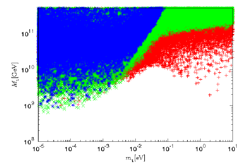
In all figures we distinguish three different kinds of points: those characterized by a strong one-flavor dominance for which or (red crosses), those characterized by a mild one-flavor dominance for which or (green x) and finally those for which a democratic scenario is realized such that (blue stars). This will make possible to understand under which circumstances the upper bound on can be evaded when flavor effects are taken into account.
In Fig. 6 the results are shown both for normal (left panel) and inverted (right panel) hierarchy and have been obtained using the approximation . One can see that there is no upper bound on , as first pointed out in [11]. The evasion of the bounds occurs in a one-flavor dominance, as expected. Note that the results have been obtained without imposing the condition of validity of the fully flavored regime Eq. (36). In the case of inverted hierarchy (right panel) the bounds do not change significantly.

In Fig. 7 we consider the special case , corresponding to in the Eq. (32). The number of free parameters gets therefore reduced to 6 (one of the PMNS phases, , is irrelevant in this model). One can see that the bounds are very similar to the general case, just slightly more stringent at large . Therefore, the special case gives an approximate condition for the saturation of the bounds in the plane.


The phases in the PMNS matrix can play a crucial role in the fully flavored regime. This was first emphasized in [10] and then analyzed in more detail in [14, 6]. Here we want to show the effects of the PMNS phases on the lower bound found in the previous figures comparing the previous results with those obtained when the PMNS phases are turned off. The result for a general matrix is not shown because it is given precisely by Fig. 6. There are indeed enough phases present in the matrix in this case to realize a strong one-flavor dominance and to saturate the general lower bound even though the PMNS phases are set to zero. The situation is different when one considers special cases like as first found in [6]. The result is shown in Fig. 8 and comparing with Fig. 7 one can see clearly that the PMNS phases are responsible for the saturation of the bounds at large . The reason is that there is in this case only one phase in the matrix, and this is not enough to fulfill the conditions for the saturation of the lower bound. Therefore, the Majorana phase and the Dirac phase play a crucial role in this case analogously to the case for inverted hierarchy, as seen in the previous subsection and recently pointed out in [46].


Let us now discuss the consequence of imposing the condition of validity of the fully flavored regime, Eq. (36). The result is shown in the left panel of Fig. 9, to be compared with Fig. 6 where the same parameters were varied but all points were kept. One notices clearly that many points at large disappear and an upper bound on , given by , appears again and is comparable to the upper bound holding in the unflavored regime, . In the case of inverted hierarchy similar results apply. However, it should be clarified that is not an upper bound on the neutrino masses but a limit of validity of the fully flavored regime. One should therefore solve more general kinetic density matrix equations in order to describe the intermediate regime and to see whether there is or not an upper bound on neutrino masses.
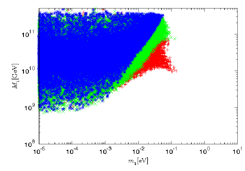
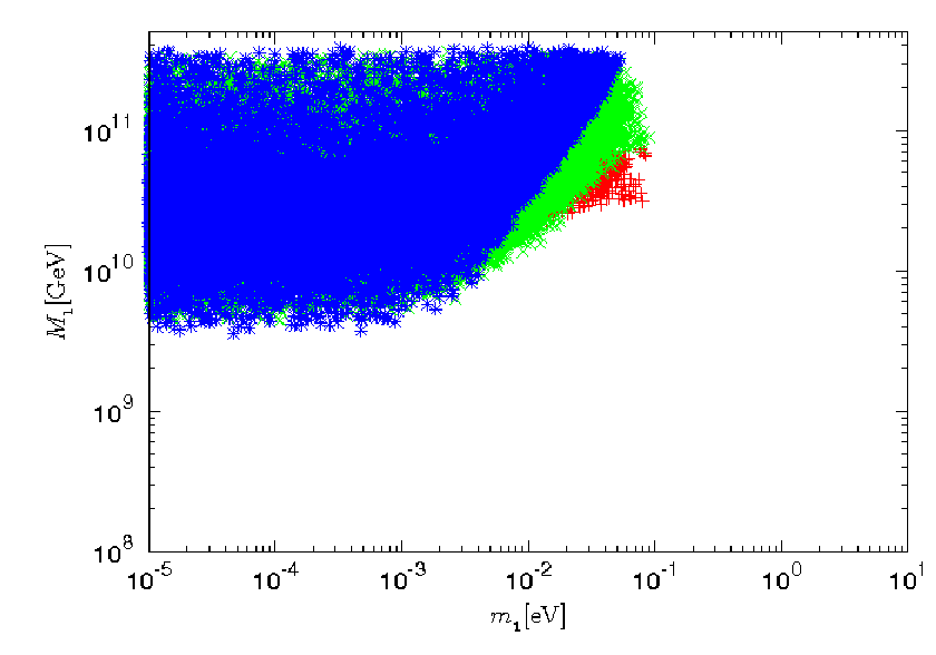
In the right panel of the same figure, we also imposed the strong washout regime condition and one can see that the allowed region gets further reduced and the upper bound on even more stringent, .
So far all results have been obtained making use of the approximation . In the upper panels of Fig. 10, left for normal hierarchy and right for inverted hierarchy, we show the results without taking into account the Higgs asymmetry solving the Eq.’s (24) neglecting in that reduces to given by the expression (25). One can see that the upper bound on gets relaxed when is neglected. In the bottom panels we used the Eq. (27) for and one can see that the results agree very well with those obtained when we used the approximation . Therefore, we will continue to use this approximation in the following analysis.


A particularly interesting case to be discussed is when all the high-energy phases are switched off, i.e. imposing the matrix to be real. In this case the PMNS phases act as the only source of violation responsible for the explanation of the observed matter-antimatter asymmetry [10]. It is therefore interesting to understand whether there is an allowed region at all [6]. The results are shown in Fig. 11 for . We show both the results obtained when both Majorana and the Dirac phase are switched on (red points) and those obtained when only the Dirac phase is non-vanishing (green points) and for , the experimental upper bound. This even more special case is the Dirac phase leptogenesis scenario [19]. The Dirac phase being the only phase that we can realistically measure in the near future in neutrino oscillation experiments, it is therefore particularly relevant to understand whether this testable source of violation can be also responsible for the observed matter-antimatter asymmetry.
The top-left panel is for normal hierarchy while the top-right is for inverted hierarchy. One can notice that in this last case the lower bound on tends to infinite for vanishing , meaning that the final asymmetry tends to vanish 11 1 Similar results have been recently obtained in [47].. In both cases there is an upper bound on , as first discussed in [17]. In the bottom-left panel we impose the condition of validity of the fully flavored regime given by the Eq. (36) and one can see that the allowed region gets reduced in a relevant way. Imposing even the strong washout regime condition (i.e. independence of the initial conditions) one can see that the allowed regions gets further reduced and it practically disappears for the case of Dirac phase leptogenesis, confirming, more generally, what was found in [19].


5.3 Effect of large values
So far, we imposed the restriction . In this subsection we relax this restriction studying the effect of allowing as large as 10 on the bounds. The main effect is that the extra-term in the flavored asymmetries (cf. Eq. (52)) can become dominant. The upper bound Eq. (55) does not apply to this term. Since this term is suppressed like the dominance is possible for a mild hierarchical spectrum, such that . In any case notice that its dominance applies under conditions that are much less restrictive than those found for the dominance of , that is suppressed like and that cancels when .


In Fig. 12 we show the allowed region in the plane for and for so that does not give any contribution. The results have to be compared with those in Fig. 4. The maximum effect is obtained again, like for , when is large. In the top panels only is allowed to be as large as 10, while . In the top-left panel and in the top-center panel, for normal and inverted hierarchy respectively and for . One can see how the lower bound on gets relaxed of one order of magnitude so that it can be as low as . Analogous relaxation applies to the lower bound on the reheat temperature . Notice that in the limit of no washout, for , the usual unflavored lower bound is recovered. In the top-right panel , such that the extra-term is suppressed enough not to be able to relax the lowest bound on . In the bottom panels we allowed to be as large as 10 while . One can see that the effect is much more reduced since now increases but at the same time and the washout increase as well.
6 On the validity of the -dominated scenario
In general, the final asymmetry receives a contribution from the decays of all 3 RH neutrinos: . In this Section we want to find a condition that guarantees the validity of the bounds within the -dominated scenario, where .
If , then the asymmetry produced from the heaviest RH neutrino decays occurs always in the unflavored regime. If moreover we impose , then it can be always safely neglected since the total asymmetry is strongly suppressed and at the same time a strong washout from and is unavoidable [5].
On the other hand, is not necessarily suppressed. A condition that guarantees the possibility to neglect in the determination of the bounds is equivalent to impose
| (58) |
From the Eq. (8) and using the orthogonal parametrization, the asymmetry can be recast as [5]
| (59) |
where we defined
| (60) |
There are two special cases for which the -dominated scenario is certainly valid. The first is to have (i.e. ), since in this case it is simple to see that . The second case is the limit . In this case is given by the Eq. (33) and it is easy to see that . This result can be understood considering that in this limit the heaviest RH neutrino decouples and so necessarily the interference term .
The opposite case is for , since now one has while
| (61) |
the same maximum value holding for (cf. Eq. (49)) but where are replaced by . Notice moreover that for one has , so that the asymmetry produced from -decays is certainly not washed out by -inverse decays. In this situation a -dominated scenario is realized, with and with no lower bound on [5].
Between these two well-defined special cases, one has to take into account both a contribution from -decays and a contribution from -decays. For example, choosing one has
| (62) |
Assuming that , such that the asymmetry from -decays is produced in the unflavored regime and that , one can see that even neglecting the washout from -inverse processes the contribution from -decays can be safely neglected in the determination of the bounds.
This example shows that if the first term in the Eq. (59) vanishes, then can be neglected in the determination of the bounds in the hierarchical limit where . Therefore, a condition certainly guarantees the validity of the -dominated scenario but is quite a restrictive one. However, this condition enlightens that an asymmetry generated from -decays requires an interference of the heaviest RH neutrino with . Indeed, as we said, this condition is certainly verified in the limit , when the heaviest RH neutrino decouples and .
Now we want to see whether, starting from , one can turn on a rotation () still having a negligible . Since both for and one has , one could naively think that this is still true for and therefore that is a sufficient condition for the validity of the -dominated scenario. However it is easy to check it is not true that and therefore it is not guaranteed that the asymmetry from -decays can be neglected. This has to be done by inspection. Since we are assuming the hierarchical limit, , the calculation of factorizes in two terms
| (63) |
The first term is the asymmetry produced at from -decays, while the second term is the washout from -inverse processes.
A precise calculation of has to take into account two types of flavor effects. If , then the asymmetry produced from -decays is fully projected on the three-flavor basis at the time when the asymmetry is washed out by -inverse processes [49]. Assuming moreover that , so that the asymmetry from decays is produced in the unflavored regime, the contribution to the final asymmetry from -decays can be calculated as
| (64) |
On the other hand, if , then the asymmetry is produced in the fully flavored regime and
| (65) |
Notice, however, that since we are interested in finding the condition for the -dominated scenario to hold, then and at the time of the washout from -inverse processes the asymmetry is projected on a two-flavor basis: the flavor and an orthogonal combination of electron and muon flavors. In this situation -inverse processes have the effect to further project the asymmetry stored in the flavor on a two-flavor basis where one direction is determined by and the other is the orthogonal component [12, 48]. The washout from -inverse decays does not touch this orthogonal component and therefore, accounting for this effect, the value of the final asymmetry has to lie somewhere between the value of the asymmetry produced at and the value of the asymmetry calculated neglecting the effect of projection along ,
| (66) |
As already mentioned, two special cases where the validity of the -dominated scenario is guaranteed are and . In Fig. 13 we show the results obtained in a more general case. We allow where but still . In the left panels we show the results in the plane . The final asymmetry is calculated both neglecting the washout (red points) and with the washout calculated in the two-flavor regime (green points) but neglecting the effect of projection of the asymmetry due to -inverse processes: as we said an account of this effect should give a result that has to be somehow in between.


One can see in the top-left panel that for the asymmetry produced by -decays falls below the observed one indicated by the horizontal solid line. Here we are imposing and we are assuming the reheat temperature to be higher than . This result can be actually also translated into a condition on the reheat temperature given by , while this time is free. The result is shown in the right panels of the same figure and one can see that the lower bound on the reheat temperature is approximately five time more relaxed compared to the lower bound on .
In the bottom panels we imposed . One can see that even for such small angles there is still a marginal allowed region. Therefore, only for very small values one recovers the special case .
This result shows that while for or for the asymmetry from -decays is always suppressed and the -dominated scenario holds, as soon as one allows either or or both, the asymmetry produced from -decays can explain the observed asymmetry for acceptable values of . Even though we did not perform a systematic calculation of the final asymmetry from -decays in the whole parameter space, in the light of this result it emerges that, if , then the -dominated scenario seems to be the most natural choice and the validity of the -dominated scenario relies on unnaturally small complex angles in order to suppress . We can therefore confirm even in a stronger way what we said in the introduction: it is misleading to talk of a lower bound on in leptogenesis, while it is more correct to talk of a lower bound on holding in the hierarchical limit for .
We also notice that this result is not relying crucially on an exact calculation of the washout from -inverse processes but more on the calculation of the asymmetry produced at . In the same Fig. 13 we show (red points) the asymmetry , without the washout, while the green points take into account the washout term calculated with the Eq. (64). We also show (blue points) the results that would have been obtained calculating the washout neglecting flavor effects.
One can see that the main result relies on the observation that is large already when small are turned on. A proper calculation of the washout is an important step but somehow a secondary one. Certainly a proper account of flavor effects greatly enhances the asymmetry from -decays but primarily it is important that there is an asymmetry to be washed out. Notice that an account of the effect envisaged in [48] would produce results somewhere in between the green and the red points. It is certainly important for a precise evaluation but it does not seem to play a crucial role.
Our results show that there is a continuous increase of the asymmetry going from , where it vanishes, toward . What is important is that as soon as one switches on small or the contribution from -decays is sufficient to explain the observed asymmetry. Going toward the case (), the allowed region for the -dominated scenario increases and the lower bound on relaxes down to a few’s [5]. We do not see any discontinuity or qualitatively different regime as envisaged in [22] where the authors distinguish a decoupled regime from a strong washout regime. A proper evaluation of the washout term , taking into account all kinds of flavor effects [49, 48] is in any case an important ingredient for a correct determination of the border between the domain of validity of the -dominated scenario and that one of the -dominated scenario.
7 Beyond the hierarchical limit
Finally, in this section we discuss how the bounds change going beyond the hierarchical limit, when . We first neglect flavor effects induced by charged lepton interactions. Notice that there is a second type of flavor effects in the heavy neutrino sector itself [12, 24, 48] due to the fact that for example the lepton quantum state produced by a RH neutrino does not coincide with produced by a RH neutrino and in particular does not in general inverse decays with a Higgs to produce a with the same rate as . We will neglect this effect that would imply that washout terms do not simply add up in the Eq. (16).
Under these assumptions, there are three different effects that change the bounds compared to the hierarchical limit [43]. First of all, in general, one cannot neglect the contribution from the heavier RH neutrinos. Therefore, one cannot just relax the assumption of hierarchical spectrum without also considering the heavier RH neutrino decays. Second, now the addition of washout in the Eq. (16) cannot be neglected. Third, the total asymmetries get typically enhanced compared to their value in the hierarchical limit. The first and third effect tend to increase the final asymmetry relaxing the bounds but the second effect tends to reduce the final asymmetry, making the bounds more stringent. The first two effects saturate for , the so called degenerate limit, and therefore when decreases below only the third effect is left and it changes the bounds in quite a simple way [43], except for some effects studied in [50] in the extreme case of resonant leptogenesis. However, notice that in the case of resonant leptogenesis the bounds simply disappear. Therefore, here we focus especially on the transition between the hierarchical limit and the degenerate limit, for . The final asymmetry is given by , where is given by the Eq.’s (37)-(40) while, from the Eq. (8), the total asymmetries and are given by
| (67) |
The unflavored efficiency factors are given by the Eq. (35) with ,
| (68) |
where we defined . Let us assume that the -abundances track closely the equilibrium value, so that . This approximation works well for , as we will assume in the following. An approximated expression for is then obtained
| (69) |
In [5, 43] it was shown that conservatively for
| (70) |
one can assume the hierarchical limit for the calculation of . In this case the washout from the RH neutrinos lighter than is factorized and (cf. Eq. (44))
| (71) |
On the other hand the washout from the -inverse processes on the asymmetry produced by -decays is negligible and
| (72) |
where with we indicated one particular . Typically one has and this is the reason why we always used as a condition for the hierarchical limit to hold. On the contrary, if , then one recovers the degenerate limit where . There are three different cases: a partial degenerate limit with , a partial degenerate limit with and a full degenerate limit where . In this last case one has simply
| (73) |
We will now focus on two particular choices for but without imposing any restriction on . The first case we consider is . This was also studied in [43] but for two particular choices of the orthogonal matrix, while here we do not make any assumption on . The contribution from the heaviest RH neutrino is negligible both because and because . The washout of -inverse processes on the asymmetry produced from the two lightest RH neutrino decays is negligible as well.
Two convenient fits for and can be used [43],
| (74) |
and
| (75) |
For the Eq. (67) for can be further specialized into
| (76) |
If and if one maximizes over the parameters, the first term can be neglected and since , the expression simplifies into
| (77) |
While gets suppressed when increases (cf. Eq. (49)), the function in general does not and therefore, at large , it gives the dominant contribution to the maximum asymmetry determining the bounds in the plane that are shown in Fig. 14 for and where we imposed a strong washout condition. This automatically guarantees the validity of the fits (74) and (75) for the efficiency factors. The results in the unflavored case correspond to the green points.


One can notice a result already found in [43] that we confirm here in a more general way. For the washout addition makes the lower bound on even slightly more stringent while only for the lower bound gets clearly more relaxed. On the other hand, concerning the upper bound on , the fact that increases with implies that the upper bound on gets relaxed already at .
Let us now turn to study the second case when . This time the heaviest RH neutrinos contribute both to the asymmetry production and to the washout. Having the expressions for the case , it is easy to derive the efficiency factors in the partial degenerate limit . Indeed if , one has simply
| (78) | |||||
The calculation of the total asymmetries and is slightly more involved. If we assume that exactly, then the interference term between and vanish, though notice that the expression Eq. (8) for and diverge for because they hold only for mass differences less than the decay widths. Therefore, one has
| (79) |
In passing let us notice that, without the interference term between and , the asymmetries vanish for . The final asymmetry can then be written as
| (81) | |||||
Notice that if , then and therefore the contribution from the two heavier RH neutrinos is suppressed as well. This makes the bounds more stringent compared to the case , especially for . In Fig. 15 we show the bounds in the case again for .


One can see that now for not only the lower bound on does not get relaxed but also the upper bound on (green points). Again, for , both the lower bound and the upper bound get clearly relaxed.
Both in the case and in the case , we repeated the calculations also in the fully flavored regime. Now the final asymmetry has to be calculated using
| (82) |
where we generalized the approximated form we already used in the hierarchical limit (cf. Eq. (50)).
In the case , the contribution from -decays is this time less trivially negligible because in principle the washout from the the two lighter RH neutrinos could be weaker in one flavor and because moreover the flavored asymmetries , contrarily to the total , are not necessarily suppressed in the hierarchical limit [6]. However, it turns out that the contribution from -decays is too small to explain the observed asymmetry and it can be therefore neglected in the determination of the bounds.
Assuming , expressions for the flavored efficiency factors can be obtained from the unflavored ones just replacing . In this way we can use the approximation (69) and the fits Eq. (74) and (75) with replaced by .
In Fig. 14 one can see how flavor effects affect the bounds (red points). For there is no relaxation of the lower bound on , since the hierarchical limit still holds and because at the onset of the strong washout there is no relaxation due to flavor effects for [6], as we are imposing. For and one can see that there is a factor two relaxation. The reason is that the asymmetry is not maximized in a one flavor dominance case but in a democratic case, that means for values of the parameters where the only change to the final asymmetry from flavor effects is described by the enhancement of a factor , while the additional terms vanish. On the other hand, for , one flavor dominance makes possible a large enhancement of the asymmetry and this is why the upper bound on is much more relaxed. Similar results hold in the case , as one can see from Fig. 15.
8 Conclusions
The simple vanilla leptogenesis scenario grasps important features of leptogenesis bounds but misses many important effects. Assuming the -dominated scenario, the lower bound on seems to be a solid feature and we have seen that it resists even for heavy neutrino mass degeneracies as small as . However, our analysis revealed that flavor effects introduce new violating terms that relax the bound of one order of magnitude for acceptable choices of the parameters and still within the hierarchical limit. Flavor effects modify the upper bound on as well but, as we stressed, an ultimate answer requires solutions of more general kinetic equations that should be able to describe the intermediate regime where the coherence of the final quantum lepton state is lost but a full decoherence is still not achieved. We have seen that an account of the Higgs asymmetry supports such a prudent conclusion.
Still within the hierarchical limit but accounting for the asymmetry produced from the -decays, the lower bound on disappears and is replaced by a lower bound on that still implies a lower bound on the reheat temperature. We showed some more general conditions for the validity of the -dominated scenario and of the lower bound on . For example the -dominated scenario certainly applies in the popular two effective RH neutrino limit, for , that implies that the heaviest RH neutrino decouples. However, apart from this case, our analysis indicates that a -dominated scenario is a more natural option and that neglecting the asymmetry from -decays can be a wrong assumption.
In conclusion, our analysis answered many different questions about the bounds on neutrino masses that are obtained within the leptogenesis scenario based on the simplest version of the see-saw mechanism. Despite many proposed extensions, this still represent the most attractive possibility since it realizes a successful link between the neutrino masses and the observed asymmetry where the measured values exhibit an interesting conspiracy. The discovery of violating effects in neutrino oscillations or in lepton decays, the determination of the absolute neutrino mass scale and of the neutrino mass spectrum ordering, normal or inverted, will likely provide further interesting tests during next years, making current experimental ‘coincidences’ even stronger or forcing departures from the minimal picture.
Acknowledgments
We wish to thank A. Riotto for many useful discussions. PDB is supported by the Helmholtz Association of National Research Centres, under project VH-NG-006.
References
- [1] M. Fukugita, T. Yanagida, Phys. Lett. B 174 (1986) 45.
- [2] P. Minkowski, Phys. Lett. B 67 (1977) 421; T. Yanagida, in Workshop on Unified Theories, KEK report 79-18 (1979) p. 95; M. Gell-Mann, P. Ramond, R. Slansky, in Supergravity (North Holland, Amsterdam, 1979) eds. P. van Nieuwenhuizen, D. Freedman, p. 315; S.L. Glashow, in 1979 Cargese Summer Institute on Quarks and Leptons (Plenum Press, New York, 1980) p. 687; R. Barbieri, D. V. Nanopoulos, G. Morchio and F. Strocchi, Phys. Lett. B 90 (1980) 91; R. N. Mohapatra and G. Senjanovic, Phys. Rev. Lett. 44 (1980) 912.
- [3] S. Davidson and A. Ibarra, Phys. Lett. B 535 (2002) 25.
- [4] W. Buchmüller, P. Di Bari and M. Plümacher, Nucl. Phys. B 643 (2002) 367.
- [5] P. Di Bari, Nucl. Phys. B 727 (2005) 318.
- [6] S. Blanchet and P. Di Bari, JCAP 03 (2007) 018.
- [7] W. Buchmüller, P. Di Bari and M. Plümacher, Annals Phys. 315 (2005) 305.
- [8] G. F. Giudice, A. Notari, M. Raidal, A. Riotto and A. Strumia, Nucl. Phys. B 685 (2004) 89.
- [9] W. Buchmuller, P. Di Bari and M. Plumacher, Nucl. Phys. B 665 (2003) 445.
- [10] E. Nardi, Y. Nir, E. Roulet and J. Racker, JHEP 0601 (2006) 164.
- [11] A. Abada, S. Davidson, F. X. Josse-Michaux, M. Losada and A. Riotto, JCAP 0604 (2006) 004
- [12] R. Barbieri, P. Creminelli, A. Strumia and N. Tetradis, Nucl. Phys. B 575 (2000) 61.
- [13] T. Endoh, T. Morozumi and Z. h. Xiong, Prog. Theor. Phys. 111 (2004) 123; A. Pilaftsis and T. E. J. Underwood, Phys. Rev. D 72 (2005) 113001 O. Vives, Phys. Rev. D 73 (2006) 073006.
- [14] A. Abada, S. Davidson, A. Ibarra, F. X. Josse-Michaux, M. Losada and A. Riotto, JHEP 0609 (2006) 010.
- [15] S. Pascoli, S. T. Petcov and A. Riotto, Phys. Rev. D 75 (2007) 083511.
- [16] S. Pascoli, S. T. Petcov and A. Riotto, Nucl. Phys. B 774 (2007) 1.
- [17] G. C. Branco, R. Gonzalez Felipe and F. R. Joaquim, Phys. Lett. B 645 (2007) 432.
- [18] S. Antusch and A. M. Teixeira, JCAP 0702 (2007) 024.
- [19] A. Anisimov, S. Blanchet and P. Di Bari, JCAP 0804 (2008) 033.
- [20] S. Blanchet, P. Di Bari and G. G. Raffelt, JCAP 03 (2007) 012.
- [21] A. De Simone and A. Riotto, JCAP 0702 (2007) 005.
- [22] S. Davidson, E. Nardi and Y. Nir, arXiv:0802.2962 [hep-ph].
- [23] K. Hamaguchi, H. Murayama and T. Yanagida, Phys. Rev. D 65 (2002) 043512.
- [24] T. Hambye, Y. Lin, A. Notari, M. Papucci and A. Strumia, Nucl. Phys. B 695 (2004) 169
- [25] S. Davidson and R. Kitano, JHEP 0403 (2004) 020.
- [26] M. C. Gonzalez-Garcia and M. Maltoni, Phys. Rept. 460 (2008) 1.
- [27] E. Komatsu et al. [WMAP Collaboration], arXiv:0803.0547 [astro-ph].
- [28] A. D. Sakharov, Pisma Zh. Eksp. Teor. Fiz. 5 (1967) 32
- [29] V. A. Kuzmin, V. A. Rubakov, M. E. Shaposhnikov, Phys. Lett. B 155 (1985) 36.
- [30] L. Covi, E. Roulet, F. Vissani, Phys. Lett. B 384 (1996) 169.
- [31] B. A. Campbell, S. Davidson, J. R. Ellis and K. A. Olive, Phys. Lett. B 297 (1992) 118; J. M. Cline, K. Kainulainen and K. A. Olive, Phys. Rev. D 49 (1994) 6394.
- [32] A. D. Dolgov and Ya. B. Zeldovich, Rev. Mod. Phys. 53 (1981) 1; E. W. Kolb and S. Wolfram, Nucl. Phys. B172 (1980) 224, ibid. B 195 (1982) 542 (E).
- [33] M. A. Luty, Phys. Rev. D 45 (1992) 455.
- [34] W. Buchmüller and M. Plümacher, Phys. Lett. B 511 (2001) 74
- [35] E. Nardi, Y. Nir, J. Racker and E. Roulet, JHEP 0601 (2006) 068
- [36] J. A. Casas and A. Ibarra, Nucl. Phys. B 618 (2001) 171.
- [37] S. Eidelman et al., Phys. Lett. B592, 1 (2004) (URL:http://pdg.lbl.gov/).
- [38] M. Fujii, K. Hamaguchi and T. Yanagida, Phys. Rev. D 65 (2002) 115012.
- [39] F. del Aguila, J. A. Aguilar-Saavedra, A. Martinez de la Ossa and D. Meloni, Phys. Lett. B 613 (2005) 170; J. Kersten and A. Y. Smirnov, Phys. Rev. D 76 (2007) 073005.
- [40] P. H. Frampton, S. L. Glashow and T. Yanagida, Phys. Lett. B 548 (2002) 119; M. Raidal and A. Strumia, Phys. Lett. B 553 (2003) 72; A. Ibarra and G. G. Ross, Phys. Lett. B 575 (2003) 279.
- [41] P. H. Chankowski and K. Turzynski, Phys. Lett. B 570 (2003) 198.
- [42] P. H. Chankowski, J. R. Ellis, S. Pokorski, M. Raidal and K. Turzynski, Nucl. Phys. B 690 (2004) 279; S. T. Petcov, W. Rodejohann, T. Shindou and Y. Takanishi, Nucl. Phys. B 739 (2006) 208.
- [43] S. Blanchet and P. Di Bari, JCAP 0606 (2006) 023.
- [44] P. Di Bari, AIP Conf. Proc. 655 (2003) 208 [arXiv:hep-ph/0211175]. P. Di Bari, [arXiv:hep-ph/0406115].
- [45] W. Buchmuller, P. Di Bari and M. Plumacher, New J. Phys. 6 (2004) 105.
- [46] E. Molinaro and S. T. Petcov, arXiv:0803.4120 [hep-ph].
- [47] E. Molinaro, S. T. Petcov, T. Shindou and Y. Takanishi, Nucl. Phys. B 797 (2008) 93.
- [48] G. Engelhard, Y. Grossman, E. Nardi and Y. Nir, Phys. Rev. Lett. 99 (2007) 081802.
- [49] O. Vives, Phys. Rev. D 73 (2006) 073006.
- [50] A. De Simone and A. Riotto, JCAP 0708 (2007) 013.