Stacks in canonical RNA pseudoknot structures

In this paper we compute the bivariate generating function

where ${\sf T}_{k,\tau}(n,t)$ is the number of $k$-noncrossing, $\tau$-canonical structures having exactly $t$ stacks. Furthermore we prove the central limit theorem

where $X_{k,\tau}^{n}$ is a random variable with distribution

see Fig. 1 and Tab. 1. Our results allow to compute the stack-numbers of a random $k$-noncrossing, $\tau$-canonical RNA structure. Since the latter are obtained via the reflection principle, it is nontrivial and currently not known how to construct such structures with uniform probability in polynomial time.

An RNA molecule is a sequence of the four nucleotides A, G, U and C together with the Watson-Crick (A-U, G-C) and (U-G) base pairing rules. RNA molecules form “helical” structures by pairing nucleotides and thereby lowering their minimum free energy (mfe). The biochemistry of these nucleotide-pairings favors parallel stacking of bonds due to mesomerie effects. The resulting $3$-dimensional configuration of the nucleotides is the RNA tertiary structure which determines the functionality of the molecule.

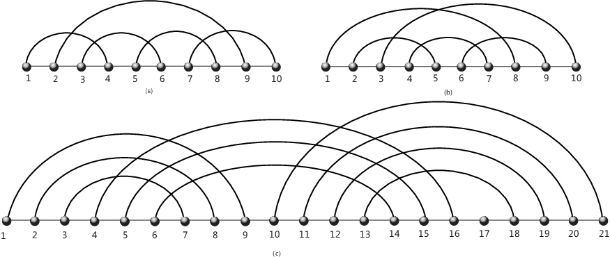
In this paper we study the distribution of stacks in $k$-noncrossing, $\tau$-canonical RNA structures. We represent RNA structures as diagrams and identify Watson-Crick (A-U, G-C) and (U-G) base pairings with arcs drawn in the upper halfplane, ignoring the bonds of the primary sequence. A diagram is a graph over the vertex set $[n]=\{1,\dots,n\}$ in which each vertex has degree less or equal to one. It is represented by drawing the vertices in a horizontal line and its arcs $(i,j)$, where $i<j$, in the upper half-plane, see Fig. 2. The vertices and arcs correspond to nucleotides and Watson-Crick (A-U, G-C) and (U-G) base pairs, respectively. Diagrams have the three key parameters $k$, $\lambda$ and $\tau$. Here $k-1$ is the maximum number of mutually crossing arcs, $\lambda$ is the minimum arc-length and $\tau$ the minimum length of a stack. A $\lambda$-arc is an arc $(i,j)$, where $j-i=\lambda$ and a stack of length $\tau$ is a sequence of “parallel” arcs: $((i,j),(i+1,j-1),\dots,(i+(\tau-1),j-(\tau-1)))$.

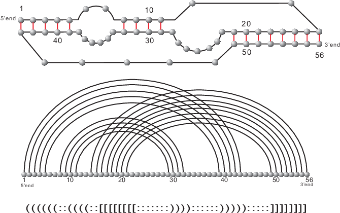
We call a $k$-noncrossing diagram with arc-length $\lambda\geq 4$ and stack-length $\tau\geq 3$ a $k$-noncrossing, $\tau$-canonical RNA structure ($\langle k,\tau\rangle$-structure). We denote the number of $\langle k,\tau\rangle$-structures and those with exactly $t$ stacks by ${\sf T}_{k,\tau}(n)$ and ${\sf T}_{k,\tau}(n,t)$, respectively. For $k=2$ this recovers the well known RNA secondary structures [6, 13, 14, 15]. Of course, the interesting cases are $k\geq 3$, where we allow for crossings, i.e. the RNA pseudoknot structures. However, to the best of our knowledge, our results are–even for RNA secondary structures new. In Fig. 3 we give two representations of a typical $\langle 3,3\langle$ RNA pseudoknot structure.

The results of this paper are relevant for the understanding of mfe RNA pseudoknot structures. Computer folding algorithms, like for instance, the dynamic programming routine of Rivas and Eddy [11], can generate, at least for $n\leq 120$, mfe-pseudoknot structures reasonably fast. While it is well known how to generate a random RNA secondary structure, the particular construction hinges on the fact that the latter can be build inductively. Although $\langle k,\tau\rangle$-structures are $D$-finite non inductive recursion exists [7, 8] and it is at present time not known how to generate them with uniform probability. Our findings are therefore of particular importance for understanding the “language of RNA”, generated by ab initio folding algorithms.

In the following, we shall identify RNA pseudoknot structures with $k$-noncrossing diagrams with minimum arc-length $\geq 4$ and stack-length $\tau\geq 3$. From now on we will always assume that any structure has a minimum arc-length greater than four. Let ${T}_{k,\tau}(n)$ (${\sf T}_{k,\tau}(n)$) denote the set (number) of $\langle k,\tau\rangle$-structures over $[n]$. Furthermore, let ${T}_{k,\tau}(n,t)$ and ${\sf T}_{k,\tau}(n,t)$ denote the set (number) of $\langle k,\tau\rangle$-structures having exactly $t$ stacks. In addition, let ${T}_{k,\tau}(n,h)$ and ${\sf T}_{k,\tau}(n,h)$ denote the set (number) of $\langle k,\tau\rangle$-structures having exactly $h$ arcs. The generating function, ${\bf T}_{k,\tau}(x)=\sum_{n\geq 0}{\sf T}_{k,\tau}(n)x^{n}$, where $k\geq 2,\,\tau\geq 3$ of $\langle k,\tau\rangle$-structures has been obtained in [10]. The function is closely related to ${\bf F}_{k}(x)=\sum_{n}f_{k}(2n)x^{2n}$, the generating function of $k$-noncrossing matchings [2]. Beyond functional equations implied directly by the reflection-principle [5], the following asymptotic formula [9] will be of importance

${\bf T}_{k,\tau}(x)$ is given as follows:

In addition we shall make use of the following basic theorem on limit distributions:

The objective of this section is to compute the bivariate generating function

For this purpose let us recall the concept of $k$-noncrossing cores developed in [8]. A $k$-noncrossing core is a $k$-noncrossing diagram in which all stacks have size one. We denote the set and the number of cores over $[n]$ by $C_{k}(n)$ and ${\sf C}_{k}(n)$, respectively. Furthermore, let $C_{k}(n,t)$ and ${\sf C}_{k}(n,t)$ denote the set and number of cores having exactly $t$ stacks. We consider the arc-sets

and set $\beta=\beta_{2}\cup\beta_{3}$. Furthermore, let

where $T_{k,1}(n,h)$ denotes the set of $k$-noncrossing diagrams without $1$-arcs having exactly $h$ arcs. We set ${\sf C}_{k}^{*}(n,0)={\sf T}_{k,1}^{*}(n,0)=1$ for $0\leq n$. In our first theorem we shall show that the number of all $\langle k,\tau\rangle$-structures with exactly $t$ stacks is a sum of the number of $C_{k}^{*}(n^{\prime},t)$-diagrams with positive integer coefficients. Let $f_{k}(m,\ell)$ denote the number of $k$-noncrossing partial matchings having exactly $\ell$ isolated points.

Proof. First, there exists a mapping from $\langle k,\tau\rangle$-structures with $t$ stacks into $C_{k}^{*}(n-2(h-t),t)$:

The core, $c(\zeta)$, is obtained in two steps: first we map arcs and isolated vertices as follows

Second we relabel the vertices of the resulting diagram from left to right in increasing order. That is we replace each stack by a single arc, keep isolated vertices and then relabel, see Fig. 4. It is straightforward to verify that $c\colon T_{k,\tau}(n,t)\rightarrow\dot{\bigcup}_{t\tau\leq h\leq\lfloor\frac{n}{2}\rfloor}\,C_{k}^{*}(n-2(h-t),t)$ is well-defined and surjective. Taking into account that each stack has its specific length gives rise to consider

given by $f_{k,\tau}(\zeta)=(c(\zeta),(\alpha_{i})_{1\leq i\leq t})$. By construction $f_{k,\tau}$ is well-defined and a bijection: obviously we can reconstruct the original $T_{k,\tau}(n,t)$-element from its core and the sequence of its stack-multiplicities (labeling the stacks from left to right). Computing the multiplicities of the resulting cores we derive

We can therefore conclude

whence eq. (10). Next we switch and consider arcs instead of stacks, using the parameter $h$. Again, collapsing the stack induces the mapping

Indeed, $c^{*}$ is well defined, since a $T_{k,1}^{*}(n,h)$-diagram can be mapped into a core structure without $1$- and $\beta$- arcs, i.e. into an element of $C_{k}^{*}(n^{\prime},h^{\prime})$. It is straightforward to show that $c^{*}$ is surjective. Labeling the $h-b$ stacks of $\zeta\in T_{k,1}^{*}(n,h)$ from left to right and keeping track of multiplicities gives rise to the map

given by $m_{k}(\zeta)=(c^{*}(\zeta),(a_{i})_{1\leq i\leq h-b})$. The mapping $m_{k}$ is well-defined and a bijection. Clearly,

and eq. (19) and eq. (20) imply

Via Möbius-inversion eq. (11) follows. It is straightforward to show that there are

ways to select $j_{1}$ $1$-arcs, $j_{2}$ $\beta_{2}$-arcs and $j_{3}$ $\beta_{3}$-arcs over $[n]$. Since removing $j_{1}$ $1$-arcs, $j_{2}$ $\beta_{2}$-arcs and $j_{3}$ $\beta_{3}$-arcs removes $2j_{1}+3j_{2}+4j_{3}$ vertices, the number of configurations of at least $j_{1}$ $1$-arcs, $j_{2}$ $\beta_{2}$-arcs and $j_{3}$ $\beta_{3}$-arcs is given by $\lambda(n,j_{1},j_{2},j_{3})f_{k}(n-2j_{1}-3j_{2}-4j_{3},n-2h-j_{2}-2j_{3})$. Via the inclusion-exclusion principle, we arrive at

whence Theorem 3.1.∎

Of course, Theorem 3.1 implies a functional relation for ${\bf T}_{k,\tau}(x,u)$:

Proof. We set

and proceed by deducing the functional equation for ${\bf T}_{k,\tau}(x,u)$ via Theorem 3.1. For this purpose we note that for $t=0$ the Binomial coefficient ${(1-\tau)t+h-1\choose t-1}$ is zero, while the term ${\sf T}_{k,\tau}(n,0)=1$ for $n\geq 1$. Clearly, ${\sf T}_{k,\tau}(n,0)=1$ counts for each $n\geq 1$ the structure consisting only of isolated vertices. We accordingly have to extend the identity of Theorem 3.1

to the case $t=0$, $n\geq 1$ which gives rise to the term $\sum_{n\geq 1}x^{n}=\frac{x}{1-x}$. Accordingly, we derive

We rewrite the right hand side of eq. (25)

Rearranging the terms of the summation we obtain

Using $\sum_{n}{{n+k}\choose n}x^{n}=\frac{1}{(1-x)^{k+1}}$, we can transform the summation over $h$ and derive

and the proof of Lemma 3.2 is complete. ∎

We next consider a functional equation for $\sum_{n,h}{\sf T}_{k}^{*}(n,h)u^{h}x^{n}$ proved in [8].

Combining Lemma 3.3 and ${\sf T}_{k,1}^{*}(n,h)=\sum_{b=0}^{h-1}{h-1\choose b}\,{\sf C}_{k}^{*}(n-2b,h-b)$ we arrive at

We shall make use of an additional relation for $\sum_{n\geq 0}\sum_{0\leq h\leq\frac{n}{2}}{\sf T}^{*}_{k,1}(n,h)u^{h}x^{n}$, proved in [10]:

We are now in the position to present the main result of this section:

Proof. We interpret the bivariate generating function

in two different ways: first, via Lemma 3.2 we have

and second according to eq. (28):

Note that, by definition of cores, we may replace the index “$h$” by “$t$” in the right hand side of eq. (34). The key observation is the relation between the terms $\frac{ux^{2(\tau-1)}}{1-x^{2}}$ and $\frac{u_{0}}{1-u_{0}x^{2}}$. Using the Ansatz

we obtain the unique solution $u_{0}=\frac{ux^{2(\tau-1)}}{1-x^{2}+ux^{2\tau}}$. Accordingly, we conclude

where $v(x)=1-x+u_{0}x^{2}+u_{0}x^{3}+u_{0}x^{4}$, and $u_{0}=\frac{ux^{2(\tau-1)}}{ux^{2\tau}-x^{2}+1}$. In order to consider eq. (30) as a relation between analytic functions we need to satisfy $ux^{2\tau}-x^{2}+1\neq 0$. Suppose $u=e^{s}$, $|s|<\epsilon$ for $\epsilon$ sufficiently small. From $|x|\leq 1/2$ and the continuity (in $s$) of the roots of the family of polynomials

we conclude $\omega_{s}(x)\neq 0$. Therefore eq. (30) holds for $u=e^{s}$, $|s|<\epsilon$ and sufficiently small $\epsilon$ and $|x|\leq 1/2$.∎

Suppose $\epsilon>0$, $2\leq k$ and $u$ is parametrized as $u=e^{s}$, where $|s|<\epsilon$. We set

We will use Theorem 3.5, which relates the generating functions ${\bf U}_{k}(z,s)$ and ${\bf F}_{k}(z)=\sum_{n}f(2n)z^{2n}$ in order to study the singularities of ${\bf U}_{k}(z,s)$.

References

• [1] E.A. Bender, Central and local limit theorems applied to asymptotic enumeration, J. Combin. Theory A. 15(1973) 91¨C111.
• [2] W.Y.C. Chen, E.Y.P. Deng, R.R.X. Du, R.P. Stanley and C.H. Yan, Crossings and Nestings of Matchings and Partitions Trans. Amer. Math. Soc. 359 (2007), No. 4, 1555–1575.
• [3] P. Flajolet, J.A. Fill, N. Kapur, Singularity analysis, Hadamard products, and tree recurrences, J. Comp Appl. Math. 174(2005) 271-313.
• [4] P. Flajolet and R. Sedgewick, Analytic combinatorics, 2007.
• [5] D.J. Grabiner, P. Magyar, Random walks in Weyl chambers and the decomposition of tensor powers, Discr. Appl. Math. 2(1993) 239-260.
• [6] J.A. Howell, T.F. Smith and M.S. Waterman, Computation of generating functions for biological molecules, SIAM J. Appl. Math. 39(1980) 119-133.
• [7] E.Y. Jin, J. Qin and C.M. Reidys, Combinatorics of RNA structures with pseudoknots Bull. Math. Biol., 70(1) (2008), 45-67.
• [8] E.Y. Jin and C.M. Reidys. RNA-LEGO: Combinatorial design of pseudoknot RNA, Adv. Appl. Math. 2008, to appear.
• [9] E.Y. Jin, C.M. Reidys and R.R. Wang, Asympotic analysis of kk-noncrossing matchings, arXiv:0803.0848 (March 2008).
• [10] Gang Ma and C.M. Reidys, Canonical RNA pseudoknot structures, arXiv:0806.2414 (June 2008).
• [11] E. Rivas, S. Eddy, A dynamic programming algorithm for RNA structure prediction inclusing pseudoknots, J. Mol. Biol. 285(1999) 2053-2068.
• [12] R. Stanley, Differentiably finite power series, Europ. J. Combinatorics. 1(1980) 175-188.
• [13] M.S. Waterman, Secondary structure of single - stranded nucleic acids, Adv. Math.I (suppl.) 1(1978) 167-212.
• [14] M.S. Waterman, Combinatorics of RNA hairpins and cloverleafs, Stud. Appl. Math. 60(1979) 91-96.
• [15] M.S. Waterman, W.R. Schmitt, Linear trees and RNA secondary structure, Discr. Appl. Math. 51(1994) 317-323.
k=2k=2 k=3k=3 k=4k=4
μk,τ\mu_{k,\tau} σk,τ2\sigma_{k,\tau}^{2} μk,τ\mu_{k,\tau} σk,τ2\sigma_{k,\tau}^{2} μk,τ\mu_{k,\tau} σk,τ2\sigma_{k,\tau}^{2}
τ=3\tau=3 0.090323 0.0189975 0.115473 0.0086760 0.123509 0.0076977
τ=4\tau=4 0.071677 0.0131316 0.086554 0.0055685 0.091737 0.0049917
τ=5\tau=5 0.059591 0.0098165 0.069467 0.0039688 0.073166 0.0035769
τ=6\tau=6 0.051092 0.0077233 0.058149 0.0026885 0.060964 0.0027313
τ=7\tau=7 0.044774 0.0062991 0.050083 0.0017584 0.052319 0.0021788
k=5k=5 k=6k=6 k=7k=7
τ=3\tau=3 0.128157 0.0070210 0.131353 0.0065187 0.133748 0.0061254
τ=4\tau=4 0.094768 0.0020037 0.119551 0.0080515 0.098461 0.0040797
τ=5\tau=5 0.075345 0.0033114 0.076864 0.0031162 0.078016 0.0029639
τ=6\tau=6 0.062629 0.0025364 0.063794 0.0023936 0.064680 0.0022823
τ=7\tau=7 0.053648 0.0020277 0.054580 0.0019171 0.055291 0.0018310