Discrete Accidental Symmetry for a Particle in a Constant Magnetic Field on a Torus
Abstract
A classical particle in a constant magnetic field undergoes cyclotron motion on a circular orbit. At the quantum level, the fact that all classical orbits are closed gives rise to degeneracies in the spectrum. It is well-known that the spectrum of a charged particle in a constant magnetic field consists of infinitely degenerate Landau levels. Just as for the and potentials, one thus expects some hidden accidental symmetry, in this case with infinite-dimensional representations. Indeed, the position of the center of the cyclotron circle plays the role of a Runge-Lenz vector. After identifying the corresponding accidental symmetry algebra, we re-analyze the system in a finite periodic volume. Interestingly, similar to the quantum mechanical breaking of CP invariance due to the -vacuum angle in non-Abelian gauge theories, quantum effects due to two self-adjoint extension parameters and explicitly break the continuous translation invariance of the classical theory. This reduces the symmetry to a discrete magnetic translation group and leads to finite degeneracy. Similar to a particle moving on a cone, a particle in a constant magnetic field shows a very peculiar realization of accidental symmetry in quantum mechanics.
1 Introduction
The fact that for some physical systems all bound classical orbits are closed leads to accidental degeneracies in the discrete energy spectrum of the corresponding quantum systems. Accidental symmetries are familiar from a particle moving in a or potential. In spatial dimensions the system then has an rotational symmetry. In case of the potential, this symmetry is dynamically enhanced to an accidental symmetry, and for the harmonic oscillator potential it is enhanced to . The accidental symmetries give rise to additional degeneracies in the discrete energy spectrum of the corresponding quantum systems, beyond the degeneracies one would expect based on rotation invariance alone [1, 2]. The components of the Runge-Lenz vector [3] are the generators of the accidental symmetry algebras. The subject of accidental symmetry has been reviewed, for example, by McIntosh [4]. Recently, we have further investigated the phenomenon of accidental symmetries, by studying a particle confined to the surface of a cone and bound to its tip by a or potential [5]. When the deficit angle of the cone is a rational fraction of , again all bound classical orbits are closed and there are accidental degeneracies in the energy spectrum of the quantum system. In this case the Runge-Lenz vector does not act as a self-adjoint operator in the domain of the Hamiltonian. Remarkably, as a consequence of this unusual property, the accidental symmetry has unusual multiplets with fractional (i.e. neither integer nor half-integer) spin.
An interesting example of an accidental symmetry involving a vector potential is cyclotron motion [6, 7]. Also in this case, there is a deep connection between the fact that all bound classical orbits are closed and additional degeneracies in the discrete energy spectrum of the corresponding quantum system. As was already noted in [7], the center of the circular cyclotron orbit is a conserved quantity analogous to the Runge-Lenz vector in the Kepler problem. Also the radius of the cyclotron orbit is a conserved quantity directly related to the energy. Interestingly, while the two coordinates of the center are not simultaneously measurable, the radius of the circle has a sharp value in an energy eigenstate. In the cyclotron problem, translation invariance disguises itself as an “accidental” symmetry. As a consequence, the symmetry multiplets — i.e. the Landau levels — are infinitely degenerate. In order to further investigate the nature of the accidental symmetry, in [8] the charged particle in the magnetic field was coupled to the origin by an harmonic oscillator potential. This explicitly breaks translation invariance and thus reduces the degeneracy to a finite amount, while rotation invariance remains intact. In this paper, we do the opposite, i.e. we explicitly break rotation invariance, while leaving translation invariance (and hence the accidental symmetry) intact by putting the system on a torus. Interestingly, the Polyakov loops, which are a consequence of the non-trivial holonomies of the torus, give rise to non-trivial Aharonov-Bohm phases which are observable at the quantum but not at the classical level. Analogous to the quantum mechanical breaking of CP invariance due to the -vacuum angle in non-Abelian gauge theories, here two self-adjoint extension parameters and explicitly break the continuous translation invariance of the classical problem down to a discrete magnetic translation group [9]. This reduces the degeneracy to a finite amount, and allows us to further investigate the nature of the accidental symmetry. In particular, just like for motion on a cone [5], symmetry manifests itself in a rather unusual way in this quantum system. In particular, due to its relevance to the quantum Hall effect, the Landau level problem has been studied very extensively (for a recent review see [10]). For example, the problem has already been investigated on a torus in [11, 12], however, without emphasizing the accidental symmetry aspects. In this paper, we concentrate entirely on those aspects, thus addressing an old and rather well-studied problem from an unconventional point of view.
The rest of the paper is organized as follows. In section 2 the cyclotron problem is reviewed in the infinite volume, with special emphasis on its oscillator algebras and accidental symmetry generators. In section 3 the system is put on a torus and the unusual manifestation of the accidental symmetry is worked out. Section 4 contains our conclusions.
2 Particle in the Infinite Volume
In this section we review the standard knowledge about a non-relativistic particle moving in a constant magnetic field in the infinite volume. We proceed from a classical to a semi-classical, and finally to a fully quantum mechanical treatment. In particular, we emphasize the symmetry aspects of the problem with a focus on accidental symmetries. This section is a preparation for the case of a finite periodic volume to be discussed in the next section. In the following, we will use natural units in which .
2.1 Classical Treatment
Ignoring its spin, we consider a non-relativistic electron of mass and electric charge moving in a constant magnetic field , which we realize through the vector potential
| (2.1) |
Since the motion along the direction of the magnetic field is trivial, we restrict ourselves to 2-dimensional motion in the --plane. Obviously, this is just standard cyclotron motion. To get started, in this subsection we treat the problem classically. The particle then experiences the Lorentz force
| (2.2) |
which forces the particle on a circular orbit of some radius . It moves along the circle with an angular velocity , which implies the linear velocity and the acceleration . Hence, Newton’s equation takes the form
| (2.3) |
with the cyclotron frequency being independent of the radius . Obviously, for this system all classical orbits are closed. The same is true for a particle moving in a or potential. In those cases, the fact that all bound classical orbits are closed is related to the conservation of the Runge-Lenz vector which generates a hidden accidental dynamical symmetry.
Let us now investigate the question of accidental symmetry for the particle in the constant magnetic field. The Lagrange function then takes the form
| (2.4) |
and the corresponding conjugate momenta are
| (2.5) |
First of all, in the gauge that we picked, is a cyclic coordinate and hence the canonically conjugate momentum is conserved as a consequence of translation invariance in the -direction. Despite the fact that the system is translation invariant also in the -direction, itself is not a cyclic coordinate and hence is not conserved. Still, using Noether’s theorem one can identify the corresponding conserved quantity as . Interestingly, the Lagrange function is not invariant under a shift in the -direction but changes by a total derivative (which leaves the classical equations of motion unchanged).
The classical Hamilton function takes the form
| (2.6) |
It is straightforward to convince oneself that has vanishing Poisson brackets, , with the three symmetry generators
| (2.7) |
One can identify , , and as the gauge-covariant generators of translations and rotations. In particular, one obtains
| (2.8) |
as one would expect for the rotation properties of the vector . As is well-known, however, in a magnetic field the two translations and do not commute, i.e.
| (2.9) |
How can these standard symmetry considerations be related to an accidental symmetry due to a Runge-Lenz vector? The Runge-Lenz vector is familiar from the Kepler problem. It points from the center of force to the perihelion position, and is conserved because all bound classical orbits are closed. Similarly, the orbit of a charged particle in a constant magnetic field is a closed circle with a fixed center. Indeed, in this case the position of this center plays the role of the conserved Runge-Lenz vector and is given by
| (2.10) |
Interestingly, the position of the center of the cyclotron circle is, at the same time, proportional to , i.e. it is orthogonal to the generators of spatial translations. Consequently, we can write
| (2.11) |
as well as
| (2.12) |
While eqs.(2.11) and (2.12) look like the usual Poisson brackets of position and momentum, one should not forget that and are just multiples of and , and should hence not be mistaken as independent variables. In particular, one also obtains the relation
| (2.13) |
Hence, just like the two generators of translations, the - and -components of the Runge-Lenz vector do not have a vanishing Poisson bracket. At the quantum level, this will imply that the - and -components of the center of a cyclotron circle are not simultaneously measurable with absolute precision.
Another conserved quantity is the radius of the circular cyclotron orbit which can be expressed as
| (2.14) |
Since is proportional to the energy, it obviously is indeed conserved.
2.2 Semi-classical Treatment
Next, we consider the same problem semi-classically, i.e. by using Bohr-Sommerfeld quantization, which, in this case, is equivalent to the quantization of angular momentum, i.e. . For a cyclotron orbit of radius , it is easy to convince oneself that
| (2.15) |
Consequently, in the semi-classical treatment the allowed radii of cyclotron orbits are now quantized. Using eq.(2.6) one finds for the energy
| (2.16) |
As is well-known, up to a constant , the semi-classically quantized energy values are those of a harmonic oscillator with the cyclotron frequency .
2.3 Quantum Mechanical Treatment
Finally, we consider the problem fully quantum mechanically. The Schrödinger equation then takes the form
| (2.17) |
We now make the factorization ansatz
| (2.18) |
and we obtain
| (2.19) |
Indeed, this is the Schrödinger equation of a shifted harmonic oscillator. Hence, the quantum mechanical energy spectrum takes the form
| (2.20) |
Interestingly, the energy of the charged particle is completely independent of the transverse momentum . As a result, the quantized Landau levels have a continuous infinite degeneracy. The energy eigenstates are shifted one-dimensional harmonic oscillator wave functions , i.e.
| (2.21) |
Similarly, one can construct eigenstates of the generator of infinitesimal translations (up to a gauge transformation) in the -direction
| (2.22) |
It is straightforward to show that the two sets of eigenstates and span the same subspace of localized states in the Hilbert space.
Since all classical orbits are closed and the center of the cyclotron orbit plays the role of a Runge-Lenz vector, it is natural to ask whether the degeneracy is caused by an accidental symmetry. Of course, since the Runge-Lenz vector plays a dual role and is also generating translations (up to gauge transformations), in this case the “accidental” symmetry would just be translation invariance. Indeed, in complete analogy to the classical case, it is easy to convince oneself that , with the Runge-Lenz vector and the angular momentum operator given by
| (2.23) |
As in the classical case, the radius of the cyclotron orbit squared is given by
| (2.24) |
and is thus again a conserved quantity. In particular, we can express the Hamiltonian as
| (2.25) |
Remarkably, although the two coordinates and of the center of the cyclotron circle are not simultaneously measurable, its radius has a definite value in an energy eigenstate.
As it should, under spatial rotations the Runge-Lenz vector indeed transforms as a vector, i.e.
| (2.26) |
These relations suggest to introduce
| (2.27) |
which implies
| (2.28) |
Hence, and act as raising and lowering operators of angular momentum. Still, it is important to note that , , and do not form an algebra. This follows because, in analogy to the classical case
| (2.29) |
i.e. and are generators of a Heisenberg algebra. As a consequence one obtains
| (2.30) |
2.4 Creation and Annihilation Operators
Since the particle in the magnetic field leads to the spectrum of a 1-dimensional harmonic oscillator (however, with infinite degeneracy), it is natural to ask how one can construct corresponding creation and annihilation operators such that
| (2.31) |
Remarkably, the creation and annihilation operators are closely related to the Runge-Lenz vector, i.e. the vector that points to the center of the classical cyclotron orbit. Since we have seen that
| (2.32) |
one is led to identify
| (2.33) |
which indeed have the desired properties. One also finds that
| (2.34) |
which implies that and also raise and lower the angular momentum. Interestingly, we have seen before that
| (2.35) |
Hence, and also act as raising and lowering operators of the angular momentum. Indeed, we can identify another set of creation and annihilation operators
| (2.36) |
which obey
| (2.37) |
As a result, raises and lowers the angular momentum by one unit. It is straightforward to derive the commutation relations
| (2.38) |
Interestingly, just like a 2-dimensional harmonic oscillator, the particle in a magnetic field is described by two sets of commuting creation and annihilation operators. However, in contrast to the 2-dimensional harmonic oscillator, the Hamiltonian of the particle in a magnetic field contains only , but not .
2.5 Alternative Representation of the Hamiltonian
Interestingly, the Hamiltonian can also be expressed as
| (2.39) |
Here we have introduced the Hamiltonian of an ordinary 1-dimensional harmonic oscillator
| (2.40) |
and the angular momentum operator has been identified as
| (2.41) |
Interestingly, the creation and annihilation operators and commute with the total energy because they raise (lower) by , while they lower (raise) by 1, such that indeed
| (2.42) |
2.6 Energy Spectrum and Energy Eigenstates
Since the algebraic structure of the problem (but not the exact form of the Hamiltonian) is the same as for the 2-dimensional harmonic oscillator, we can construct the physical states accordingly. First of all, we construct a state that is annihilated by both and , i.e.
| (2.43) |
Then we define states
| (2.44) |
which are eigenstates of the total energy
| (2.45) |
as well as of the angular momentum
| (2.46) |
It should be noted that the quantum number (which determines the energy) is non-negative, while the quantum number (which determines the angular momentum) is an arbitrary integer. The infinite degeneracy of the Landau levels is now obvious because states with the same but different values of have the same energy.
One may wonder why in subsection 2.3 we found an infinite degeneracy labeled by the continuous momentum and now we only find a countable variety of degenerate states (labeled by the integer ). This apparent discrepancy is due to the implicit consideration of two different Hilbert spaces. While the states in the discrete variety labeled by are normalizable in the usual sense, the continuous variety of plane wave states labeled by is normalized to -functions and thus belongs to an extended Hilbert space.
It is remarkable that a quantum mechanical system containing just a single particle has an even infinitely degenerate ground state. The existence of infinitely degenerate ground states is usually associated with the spontaneous breakdown of a continuous global symmetry in systems with infinitely many degrees of freedom. Does the infinite degeneracy of the single-particle Landau levels have anything to do with the spontaneous breakdown of translation invariance? The usual breaking of a continuous global symmetry is associated with the occurrence of massless Goldstone bosons. For example, when translation invariance is spontaneously broken by the formation of a crystal lattice, phonons arise as massless excitations. In the quantum mechanical system studied here, there is no room for phonons because it has only a finite number of degrees of freedom. Indeed, the infinitely degenerate ground states are separated from the rest of the spectrum by a gap . Still, just like a system with spontaneous symmetry breaking, the charged particle in a magnetic field may chose spontaneously from a continuous variety of degenerate ground states.
2.7 Coherent States
Coherent states are well-known from the harmonic oscillator, and have also been constructed for the Landau level problem [13]. As usual, the coherent states are constructed as eigenstates of the annihilation operators, i.e.
| (2.47) |
In coordinate space, the coherent states can be expressed as
| (2.48) |
Some expectation values in the coherent state are given by
| (2.49) |
Here describes the quantum uncertainty. In all cases is proportional to or , which implies that the relative uncertainty goes to zero in the classical limit.
Just as in the ordinary harmonic oscillator, the time-dependent Schrödinger equation with an initial coherent state is (up to an irrelevant phase) solved by with
| (2.50) |
As expected, the state remains coherent during its time-evolution. In particular, this implies
| (2.51) |
Hence, the coherent state represents a Gaussian wave packet moving around a circular cyclotron orbit just like a classical particle. This is obvious from the coordinate representation of the probability density
| (2.52) |
It is interesting to note that the coherent states with (but with arbitrary form an overcomplete set of degenerate ground states with the energy . These states represent Gaussian wave packets centered at the points determined by . Unlike for a free particle, these Gaussian wave packets do not spread. Semi-classically speaking, the charged particle is in a “circular orbit” of quantized sharp radius with an uncertain position of the center. Since the ground state is infinite degenerate, the charged particle can spontaneously select any average position at which it can stay with average velocity zero in a state of minimal uncertainty. Again, this is reminiscent of the spontaneous breakdown of translation invariance.
3 Particle on a Torus
In this section we put the problem in a finite periodic volume. This explicitly breaks rotation invariance, but leaves translation invariance intact (at least at the classical level), and leads to an energy spectrum with finite degeneracy. In order to clarify some subtle symmetry properties, we also discuss issues of Hermiticity versus self-adjointness of various operators.
3.1 Constant Magnetic Field on a Torus
In this subsection we impose a torus boundary condition over a rectangular region of size . This will lead to a quantization condition for the magnetic flux. Since the magnetic field is constant, it obviously is periodic. On the other hand, the vector potential of the infinite volume theory , obeys the conditions
| (3.1) |
As a gauge-dependent quantity, the vector potential is periodic only up to gauge transformations, i.e.
| (3.2) |
The gauge transformations and are transition functions in a fiber bundle which specify the boundary condition. In our case the transition functions are given by
| (3.3) |
Besides the field strength, gauge theories on a periodic volume possess additional gauge invariant quantities — the so-called Polyakov loops — which arise due to the non-trivial holonomies of the torus. For an Abelian gauge theory the Polyakov loops are defined as
| (3.4) |
In our case, they are given by
| (3.5) |
In order to respect gauge invariance of the theory on the torus, under shifts the wave function must also be gauge transformed accordingly
| (3.6) |
The angles and parametrize a family of self-adjoint extensions of the Hamiltonian on the torus. Applying the boundary conditions from above in two different orders one obtains
| (3.7) | |||||
Hence, consistency of the boundary condition requires
| (3.8) |
The total magnetic flux through the torus
| (3.9) |
is hence quantized in integer units of the elementary magnetic flux quantum . Interestingly, the spectrum of a charged particle in a constant magnetic field is discrete (but infinitely degenerate) already in the infinite volume. As we will see, in the finite periodic volume it has only a finite -fold degeneracy determined by the number of flux quanta.
A quantum mechanical charged particle is sensitive to the complex phases defined by the Polyakov loops
| (3.10) |
which are measurable in Aharonov-Bohm-type experiments. Remarkably, the Polyakov loops explicitly break the translation invariance of the torus at the quantum level. This is reminiscent of the quantum mechanical breaking of CP invariance due to the -vacuum angle in non-Abelian gauge theories. The complex phases from above are invariant under shifts by integer multiples of
| (3.11) |
in the - and -directions, respectively. Hence, at the quantum level the continuous translation group of the torus is reduced to a discrete subgroup which plays the role of the accidental symmetry group.
In this paper, we treat the gauge field as a classical background field, while only the charged particle is treated quantum mechanically. It is interesting to note that, once the gauge field is also quantized, the transition functions and become fluctuating physical degrees of freedom of the gauge field. Still, as a consequence of
| (3.12) | |||||
and of
| (3.13) | |||||
the transition functions must obey the cocycle consistency condition
| (3.14) |
In this case, the magnetic flux specifies a super-selection sector of the theory. Analogous to the center symmetry of non-Abelian gauge theories on a -dimensional torus [14, 15], Abelian gauge theories coupled to charged matter have a global center symmetry. The self-adjoint extension parameters and then turn into conserved quantities (analogous to Bloch momenta) of the global symmetry on the 2-dimensional torus. In this sense, and are analogous to the -vacuum angle of non-Abelian gauge theories, which also distinguishes different super-selection sectors of the theory. The -vacuum angle is a quantum mechanical source of explicit CP violation. At the classical level, on the other hand, CP invariance remains intact because does not affect the classical equations of motion. Similarly, for a charged particle on the torus the angles and characterize the explicit breaking of continuous translation invariance down to a discrete subgroup. Just like CP invariance for a non-Abelian gauge theory, for a charged particle on the torus the full continuous translation symmetry remains intact at the classical level, because and do not appear in the classical equations of motion.
In this paper, we treat the charged particle as a test charge which does not surround itself with its own Coulomb field. This would change, once one would derive the charged particle from its own quantum field. For example, if one considers full-fledged QED, a single electron cannot even exist on the torus because the Coulomb field that surrounds it is incompatible with periodic boundary conditions. Indeed, as a consequence of the Gauss law, the total charge on a torus always vanishes. To cure this problem, one could compensate the charge of the electron by a classical background charge homogeneously spread out over the torus. In our present calculation this is not necessary, because the charged particle is treated as a test charge without its own surrounding Coulomb field.
3.2 Discrete Magnetic Translation Group
As we have seen, in order to respect gauge invariance, on the torus the wave function must obey eq.(3.6), which can be re-expressed as
| (3.15) |
It is interesting to note that a factorization ansatz for the wave function as in eq.(2.18) is inconsistent with the boundary condition. Let us consider the unitary shift operator generating translations by a distance in the -direction as well as a -dependent phase-shift
| (3.16) |
which acts as
| (3.17) |
Obviously, commutes with the Hamiltonian because does. Indeed, the shifted wave function does obey the boundary condition eq.(3.15), i.e.
| (3.18) | |||||
which is the case only because
| (3.19) |
Furthermore, we also have
| (3.20) | |||||
Hence, as we argued before, the translations in the -direction are reduced to the discrete group . In particular, all translations compatible with the boundary conditions can be expressed as the -th power of the elementary translation . According to eq.(2.10), , such that
| (3.21) |
Similarly, up to gauge transformations the operator
| (3.22) | |||||
generates translations in the -direction. Since on the torus the Runge-Lenz vector component , which determines the -coordinate of the center of the cyclotron orbit, is defined only modulo , it is indeed natural to consider the translation operator . In fact, although it formally commutes with the Hamiltonian, the operator itself is no longer self-adjoint in the Hilbert space of wave functions on the torus. The operator , on the other hand, does act as a unitary operator in the Hilbert space. It is worth noting that, at least in the gauge we have picked, the operator is still self-adjoint. However, this would not be the case, for example, in the symmetric gauge, and it is hence most natural to work with and instead of and or equivalently and .
The boundary condition of eq.(3.15) can now be expressed as
| (3.23) |
As a consequence of the commutation relation , one obtains
| (3.24) |
This implies that
| (3.25) |
i.e., up to a periodic gauge transformation , translates the wave function by a distance .
Remarkably, although at the classical level the torus has two continuous translation symmetries, the corresponding infinitesimal generators and are not self-adjoint in the Hilbert space of wave functions on the torus. Only the finite translations and are represented by unitary operators, which, however, do not commute with each other. The two operators and generate a discrete translation group consisting of the elements
| (3.26) |
The group multiplication rule takes the form
| (3.27) |
with all summations being understood modulo . Obviously, the unit element is represented by
| (3.28) |
while the elements
| (3.29) |
form the cyclic Abelian subgroup . The inverse of a general group element is given by
| (3.30) |
because
| (3.31) |
It is interesting to consider the conjugacy class of a group element which consists of the elements
| (3.32) |
In particular, as one would expect, the elements are conjugate only to themselves and thus form single-element conjugacy classes. Obviously, multiplication by a phase is just a global gauge transformation and thus leaves the physical state invariant. Hence, the conjugacy classes correspond to gauge equivalence classes.
The elements commute with all other elements and thus form the center of the group . Since the individual elements of the center form separate conjugacy classes, the center is a normal subgroup and can hence be factored out. The center itself represents global phase transformations of the wave function, and hence factoring it out corresponds to identifying gauge equivalence classes. Physically speaking, the quotient space corresponds to discrete translations up to gauge transformations. It should be pointed out that is not simply given by the direct product . In fact, the quotient space is not a subgroup of , and hence is also not the semi-direct product of and . All we can say (besides defining the group as done before) is that it is a particular central extension of by the center subgroup .
3.3 Spectrum and Degeneracy on the Torus
Let us first discuss the classical problem on the torus. In that case, the magnetic flux need not be quantized. Also the values of the Polyakov loop are not detectable at the classical level because they have no effect on the motion of a test charge, which is entirely determined by the Lorentz force. The classical orbits of a charged particle in a constant magnetic field on the torus still are closed circles. However, as illustrated in figure 1, the circle may close only after wrapping around the periodic boundary.

Since all classical orbits are still closed, one expects that on the torus the accidental symmetry is still present.
It should be pointed out that on the torus the Hamiltonian is identically the same as in the infinite volume. It now just acts on the restricted set of wave functions obeying the boundary condition eq.(3.15). In particular, the finite volume wave functions are appropriate linear combinations of the infinitely many degenerate states of a given Landau level. As a result, the energy spectrum remains unchanged, but the degeneracy is substantially reduced.
Let us use the fact that commutes with the Hamiltonian to construct simultaneous eigenstates of both and . Since for states on the torus , the eigenvalues of are given by with , while the eigenvalues of are still given by . Hence, we can construct simultaneous eigenstates such that
| (3.33) |
The states are the finite-volume analog of the states of eq.(2.21) with . In coordinate representation these states are given by the wave functions
| (3.34) | |||||
As a special case, let us consider the ground state for , which is non-degenerate
| (3.35) | |||||
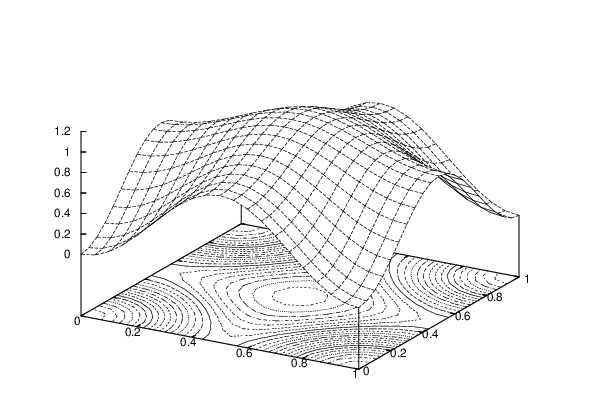
In this state the probability density, which is illustrated in figure 2, has its maximum at . This shows once again that the self-adjoint extension parameters and indeed explicitly break translation invariance.
As a consequence of eq.(3.24) one obtains
| (3.36) |
from which we conclude that
| (3.37) |
Since , the states with thus form an irreducible representation of the magnetic translation group. Using as a concrete example, a matrix representation of the two generators of is given by
| (3.38) |
Similarly, one can construct simultaneous eigenstates of and
| (3.39) |
The states are the finite-volume analog of the states of eq.(2.22) with . In coordinate representation these states are given by the wave functions
| (3.40) | |||||
It is worth noting that
| (3.41) |
Similar to the infinite volume case, it is straightforward to show that the two sets of eigenstates and span the same subspace of the Hilbert space. In particular, for the ground state is non-degenerate and one can show that
| (3.42) |
As we have seen, on the torus continuous translation invariance is explicitly broken down to the discrete magnetic translation group by the self-adjoint extension parameters and . Still, all states (including the ground state) remain degenerate. However, unlike in the infinite volume, the degeneracy is reduced to a finite amount . Only when one varies and one recovers the infinite degeneracy of the infinite system. As in the infinite volume, one may ask if the degenerate ground state indicates that the discrete magnetic translation group is spontaneously broken. While there are striking similarities with spontaneous symmetry breaking, there are also important differences. First of all, when a system with a broken symmetry is put in a finite volume, the symmetry is usually restored dynamically. For example, this is the case for the spontaneously broken chiral symmetry in QCD as well as for the spontaneously broken spin symmetry in antiferromagnets. An important exception are ferromagnets for which the ground state remains exactly degenerate even in a finite volume. This is a consequence of the fact that the magnetization order parameter of a ferromagnet is a conserved quantity, while the staggered magnetization order parameter of an antiferromagnet is not conserved. In this sense, the charged particle in a magnetic field behaves like a ferromagnet. The “order parameter” that signals the “spontaneous breakdown” of translation invariance is the Runge-Lenz vector pointing to the center of the cyclotron circle, which is indeed a conserved quantity.
3.4 Coherent States on the Torus
It is interesting to construct coherent states for the particle on the torus. This is achieved by superposition of shifted copies of the coherent state of the system in the infinite volume
| (3.43) |
By construction, this state obeys the boundary condition eq.(3.23). The factor is determined from the normalization condition
| (3.44) | |||||
It is easy to see that a finite-volume coherent state remains coherent during the time-evolution. Just as in the infinite volume, , while is time-independent. In the infinite volume determines the position of the center of the cyclotron circle. On the torus, this center is well-defined only up to shifts by multiples of or . Indeed one finds
| (3.45) |
which shows that (together with and ) the expectation values and of the infinite volume coherent state determine the position of the center of the cyclotron circle (the Runge-Lenz vector) modulo the periodicity lengths and of the torus. The prefactors in eq.(3.45) take the form
Finally, let us consider the coherent states with but arbitrary . Just as in the infinite volume, these states are ground states with minimal energy . Indeed, for (i.e. when there is no degeneracy) one can show that
| (3.47) |
(provided that the arbitrary complex phase of is chosen appropriately).
4 Conclusions
We have re-investigated an old and rather well-studied problem in quantum mechanics — a charged particle in a constant magnetic field — from an unconventional accidental symmetry perspective. The fact that all classical cyclotron orbits are closed circles identifies the center of the circle as a conserved quantity analogous to the Runge-Lenz vector of the Kepler problem. Remarkably, (up to gauge transformations) the corresponding “accidental” symmetry is just translation invariance. In particular, the coordinates of the center of the cyclotron circle simultaneously generate infinitesimal translations and (up to gauge transformations) in the - and -directions, respectively. As is well-known, in a constant magnetic field translations in the - and -directions do not commute, i.e. , and thus the two coordinates and of the center of the cyclotron circle are also not simultaneously measurable at the quantum level. In contrast, the radius of the cyclotron circle has a sharp value in an energy eigenstate. The accidental symmetry leads to the infinite degeneracy of the Landau levels.
In order to further investigate the nature of the accidental symmetry, we have put the system in a finite rectangular periodic volume. Obviously, this breaks rotation invariance, but leaves translation invariance (and thus the accidental symmetry) intact — at least at the classical level. Interestingly, at the quantum level continuous translation invariance is explicitly broken down to a discrete magnetic translation group, due to the existence of two angles and which parametrize a family of self-adjoint extensions of the Hamiltonian on the torus. In a field theoretical context, in which the gauge field is dynamical (and not just treated as a classical background field), the parameters and characterize super-selection sectors. In this sense, they are analogous to the vacuum angle of non-Abelian gauge theories. Just as the -vacuum angle explicitly breaks CP invariance at the quantum level but is classically invisible, the angles and lead to a quantum mechanical explicit breaking of continuous translation invariance down to the discrete magnetic translation group. The magnetic translation group itself, which plays the role of the accidental symmetry in the periodic volume, is a particular central extension of by the center subgroup , where is the number of magnetic flux quanta trapped in the torus. We find it remarkable that the simple fact that all classical cyclotron orbits are closed circles has such intricate effects at the quantum level.
We have also discussed the relation of ground state degeneracy with the possible spontaneous breakdown of translation invariance. Indeed the Runge-Lenz vector (which points to the center of the cyclotron orbit) acts as a corresponding “order parameter”. Just like the magnetization in a ferromagnet (but unlike the staggered magnetization in an antiferromagnet), the Runge-Lenz vector is a conserved quantity. Consequently, the ground state remains degenerate even in a finite volume. Furthermore, just as the three components of the magnetization vector do not commute with each other, the two components of the Runge-Lenz vector are also not simultaneously measurable. Still, unlike a ferromagnet, a single charged particle in a magnetic field has just a finite number of degrees of freedom and can thus not display all features usually associated with spontaneous symmetry breaking. In particular, in the system discussed in this paper there is no room for massless Goldstone excitations.
While many aspects of the Landau level problem are well-known, we hope that we have painted a picture of cyclotron motion that reveals new aspects of this fascinating system, which behaves in a unique and sometimes counter-intuitive manner.
Acknowledgments
We like to thank Nathan Habegger for an illuminating discussion about the theory of discrete groups. This work is supported in parts by the Schweizerischer Nationalfonds.
References
- [1] V. Fock, Z. Physik 98 (1935) 145.
- [2] V. Bargmann, Z. Physik 99 (1936) 576.
- [3] W. Lenz, Z. Physik 24 (1924) 197.
- [4] H. V. McIntosh, in Group Theory and its Applications, Vol. 2 (1971) 75, Academic Press, Inc. New York and London.
- [5] M. H. Al-Hashimi and U.-J. Wiese, Ann. Phys. 323 (2008) 82.
- [6] L. D. Landau, Z. Physik 64 (1930) 629.
- [7] M. H. Johnson and B. A. Lippmann, Phys. Rev. 76 (1949) 828.
- [8] V. A. Dulock and H. V. McIntosh, J. Math. Phys. 7 (1966) 1401.
- [9] J. Zak, Phys. Rev. 134 (1964) A1602.
- [10] A. Stern, Ann. Phys. 323 (2008) 204.
- [11] G.-H. Chen, L.-M. Kuang, and M.-L. Ge, Phys. Rev. B53 (1996) 9540.
- [12] H. Zainuddin, Phys. Rev. D40 (1989) 636.
- [13] A. Feldman and A. H. Kahn, Phys. Rev. B12 (1970) 4584.
- [14] G. ’t Hooft, Nucl. Phys. B153 (1979) 141.
- [15] G. ’t Hooft, Commun. Math. Phys 81 (1981) 267.