A Markov Chain Monte Carlo Algorithm for analysis of low signal-to-noise CMB data
Abstract
We present a new Monte Carlo Markov Chain algorithm for CMB analysis in the low signal-to-noise regime. This method builds on and complements the previously described CMB Gibbs sampler, and effectively solves the low signal-to-noise inefficiency problem of the direct Gibbs sampler. The new algorithm is a simple Metropolis-Hastings sampler with a general proposal rule for the power spectrum, , followed by a particular deterministic rescaling operation of the sky signal, . The acceptance probability for this joint move depends on the sky map only through the difference of ’s between the original and proposed sky sample, which is close to unity in the low signal-to-noise regime. The algorithm is completed by alternating this move with a standard Gibbs move. Together, these two proposals constitute a computationally efficient algorithm for mapping out the full joint CMB posterior, both in the high and low signal-to-noise regimes.
Subject headings
cosmic microwave background — cosmology: observations — methods: numericalI. Introduction
Since the detection of anisotropy in the Cosmic Microwave Background (CMB; Smoot et al. 1992), there has been an emphasis on likelihood or Bayesian methods for the inference of cosmological parameters and their error bars, or more generally, their confidence intervals. CMB analysis is most suitably addressed in a Bayesian, as opposed to frequentist, framework, simply because the observed microwave sky is interpreted as a single realization of a spatial random process.
Early measurements of the CMB were limited to signal to noise ratios of order unity at relatively low angular scales, where direct evaluation of the likelihood for the power spectrum or cosmological parameters is possible. However, the scaling of computational expense with pixel number prohibits direct likelihood evaluation for current and future CMB observations. Motivated by the scientific potential of CMB data with increasingly high spatial resolution, yet beset with systematics including partial sky coverage and foregrounds, an iterative method of sampling from the Bayes posterior, using a special case of Markov Chain Monte Carlo (MCMC) known as Gibbs sampling, was introduced by [18, 19]. The method was later independently discovered and applied to COBE data [29], numerically extended to high-resolution on the sphere [4], applied to analysis of the WMAP [2, 15, 24] data [23, 5, 6], as well as generalized to include inference of foreground model parameters [7, 8].
While Gibbs sampling provably converges to the Bayes posterior over the entire range of angular scales probed by the data, the run-time required to generate enough independent samples at the low signal-to-noise, small angular scale regime was found to be prohibitive [4]. The reason for this is that typical variations in the power spectrum from one sample to the next are determined by cosmic variance alone, whereas the posterior itself is given by both cosmic variance and noise. This results in a long correlation length in the sequence of spectra in the low signal to noise regime, thus requiring a very long run time to generate a sufficient number of independent samples.
In this paper we generalize the original Gibbs sampling algorithm to include a new type of MCMC step alternating with standard Gibbs sampling, which solves this problem of slow probabilistic convergence in the low signal to noise regime. This method therefore makes possible an exact Bayesian approach to CMB analysis over the entire range of angular scales probed by current and future experiments.
The paper is organized as follows. We first review the CMB Gibbs sampler, and describe the associated numerical difficulties in analysis at small angular scales. We then introduce the new MCMC step to the Markov chain, designed specifically to allow large variations in the high- CMB spectrum, precisely where the signal to noise is . We derive the required Metropolis-Hastings acceptance probability correctness in Appendix A, and numerically demonstrate the method in Section IV, for both temperature and polarization. Finally, we summarize and conclude in Section V.
II. Review of Gibbs Sampling
II.1. The Joint Posterior
We begin by assuming that the observed data may be modelled by a signal and a noise term,
| (1) |
where is a vector containing the data (at every pointing of the detectors), the matrix involves both pointing and beam convolution (and where for this paper we will assume symmetric beams and neglect the details of this operation), and is additive noise (here in the pixel domain). We assume both the CMB signal and noise to be Gaussian random fields with vanishing mean and covariance matrices and , respectively. In harmonic space, where , the CMB temperature covariance matrix is given by , being the angular power spectrum. A generalization to polarization merely requires the replacement of the signal matrix diagonal elements with matrices of the form
| (2) |
For the discussion in this section, we focus on the temperature case, but note that the generalization to polarization is straightforward and discussed by Larson et al. [21].
Given these asumptions, our goal is to quantify what has been learned about the underlying power spectrum of the CMB given the data, or how well the data constrain the cosmological parameters. One proceeds then, in a Bayesian framework, by writing down the posterior given the data,
| (3) |
Here is the likelihood and is a prior on .
In order to derive the functional form of the likelihood, one imagines randomly choosing any relevant model [here a power spectrum drawn from ], and asks what sequence of effects needs to be modeled in order to simulate the data. Here, simulation is understood as conditioning on the chosen model, and leads to a joint density
| (4) | |||||
where the last line follows directly from our data model through the assumption of additive noise. Specifically, the factors in the above are
| (5) |
which follow from the assumption that both the signal and noise are independent Gaussian processes.
The idea of a “simulation chain” provides a conceptually clear approach to constructing a joint density, from which we immediately have the Bayesian posterior
| (6) |
The relevance of the above for this paper lies in relating what we refer to as the joint posterior, , and the more familiar likelihood ,
Although we can analytically compute the integral of the joint posterior over the signal for the Gaussian signal and noise processes considered here, and therefore simply write down the functional form of the likelihood, it is too expensive to evaluate it for any specified given high-resolution data. Furthermore, for more complicated data models (i.e. including foreground model uncertainties) we will not be able to perform the integrals over the additional degrees of freedom. Both situations then instead motivate sampling from the joint posterior, and thereby generating samples from without ever evaluating . We now discuss the original Gibbs sampling approach proposed and implemented by Jewell et al. [19], Wandelt et al. [29] and Eriksen et al. [4], and then introduce a new MCMC step which directly addresses the previously reported slow probabilistic convergence in the low signal to noise regime [4].
II.2. The CMB Gibbs sampler
As stated above, our goal is to sample from the joint posterior,
| (7) |
For notational convenience, we have here dropped constant factors of , and also defined
| (8) |
One approach to sample from this posterior is to use an algorithm known as Gibbs sampling, where we can alternately sample from the respective conditional densities,
| (9) | ||||
| (10) |
Here indicates sampling from the distribution on the right-hand side. After some burn-in period, during which all samples must be discarded, the joint samples will be drawn from the desired density. Thus, the problem is reduced to that of sampling from the two conditional densities and .
We now describe the sampling algorithms for each of these two conditional distributions, starting with . First, note that which follows directly from the construction of the joint density of “everything” above. This is also intuitively easy to understand since if we already know the CMB sky signal, the data themselves tell us nothing new about the CMB power spectrum. Next, since the sky is assumed to be Gaussian and isotropic, the distribution reads
| (11) |
which, when interpreted as a function of , is known as the inverse Gamma distribution. In this expression, denotes the observed power spectrum of . Fortunately, there exists a simple textbook sampling algorithm for this distribution [14, e.g.,], and we refer the interested reader to the previous papers for details. For an alternative, and more flexible, sampling algorithm, see Eriksen & Wehus [9].
In order to describe the sky signal sampling step, we first define the mean-field map (or Wiener filtered data) to be , and note that the conditional sky signal density given the data and can be written as
| (12) |
Thus, is a Gaussian distribution with mean equals to and a covariance matrix equals to .
Sampling from this Gaussian distribution is straightforward, but computationally somewhat cumbersome. First, draw two random white noise maps and with zero mean and unit variance. Then solve the equation
| (13) |
for . Since the white noise maps have zero mean, one immediately sees that , while a few more calculations show that .
The problematic part about this sampling step is the solution of the linear system in Equation 13. Since this a system for current CMB data sets, it cannot be solved by brute force. Instead, one must use a method called Conjugate Gradients (CG), which only requires multiplication of the coefficient matrix on the left-hand side, not inversion. For details on these computations, together with some ideas on preconditioning, see Eriksen et al. [4].
II.3. Convergence issues in the low signal-to-noise regime
As originally applied to high-resolution CMB data, the Gibbs sampling algorithm as described above has very slow convergence at the high-, low signal-to-noise part of the spectrum. The reason for the slow convergence is easy to understand in light of the above: When sampling from , the typical step size is given by cosmic variance at all angular scales. In the high signal-to-noise regime, cosmic variance dominates the noise variance, and we are able to explore the full width of the posterior in only a few Gibbs iterations. However, in the low signal-to-noise end, cosmic variance is far smaller than the posterior variance, and it takes a prohibitively long time to converge probabilistically. This problem of “slow mixing” of the Gibbs sampler is illustrated in figures 1 and 2. The long correlation length starting at signal-to-noise of unity leads to extremely long run times in order to produce a reasonable number of uncorrelated samples.
III. A Low Signal-to-Noise MCMC Sampler
When sampling from the true posterior, the goal is to produce as many independent samples from as possible. One might intuitively guess that it should be straightforward to establish good approximations to the posterior in the low signal-to-noise regime, since in the limit of vanishing signal to noise we simply recover the prior. This suggests that we look for a sampling scheme in which we first sample a new spectrum from some approximation to the true posterior independent on the current spectrum and CMB map, followed by sampling the CMB map from the conditional . The problem with such a direct scheme is that the accept probability will involve a ratio of determinants which are too expensive to compute.
We are therefore motivated to look for a sampling scheme in which we can make a large variation in in the low signal-to-noise regime, and make an associated deterministic change in the CMB map, while still maintaining a reasonably high acceptance rate. The motivation for a deterministic change is that it will avoid introducing ratios of determinants which we cannot compute.
III.1. Proposal rule and acceptance probability
Assume that we have defined a deterministic sampling scheme for , and that our new CMB map is given by some function
| (14) |
Then the condition of detailed balance for our MCMC sampler requires that
| (15) |
or, in other words, that the inverse function is given by exchanging the order of the spectra in the function . One simple function which has this property is
| (16) |
The total proposal matrix is then
and the “reverse” proposal is
The condition of detailed balance including deterministic moves requires the consideration of some technical points which we leave to Appendix A. There we show that the full Metropolis-Hastings accept probability reads
| (17) |
The significance of the above is that we can make relatively large changes to the power spectrum in the low signal-to-noise regime, where is getting small, since the is affected only very mildly by changes in any low signal-to-noise mode.
We note the interesting point (discussed more completely in Appendix B) that if one changes variables in the joint posterior from CMB maps, , to whitened maps, , and then Gibbs sample in the new variables , the resulting accept probability is numerically identitical to the above. However, we note the distinction here to emphasize the difference between MCMC algorithms implementing deterministic proposals of maps given , and those sampling in a different set of variables, as there could be other deterministic proposal schemes or another change of variables which lead to improvements over the approach presented in this paper.
For the numerical demonstration of the MCMC algorithm presented in this paper, we use a simple symmetric Gaussian proposal, truncated at (or, for polarization, the region where the resulting CMB covariance matrix is positive definite), for the power spectrum,
| (18) |
where is a measure of the typical step size taken between two samples. Note that because this proposal density is symmetric, the ratio of proposals cancels, and the acceptance probability is entirely determined by the change in .
It should be noted that while the above MCMC step satisfies detailed balance, it is not irreducable, in the sense that there is not a non-vanishing probability in reaching any state from any other state in a finite number of MCMC steps; the phases are unchanged in each MCMC step. However, alternating these steps with a traditional Gibbs sampling step gives a combined “two-step” MCMC algorithm which indeed is irreducable, and therefore provably converges to the joint posterior. Once again, the details are left to the appendix for the interested reader.
III.2. Optimization of the MCMC sampler
A general advantage of the Gibbs sampler is the fact that it is free of tunable efficiency parameters. The same is not true for the Metropolis-Hastings MCMC algorithm; for satisfactory sampling performance, it typically has to be tuned quite extensively. In this section, we describe three specific features that helps in this task, namely 1) step size tuning, 2) slice sampling and 3) binning.
First, we have to ensure that the step size of our Gaussian proposal density roughly matches the width of the target distribution, in order to maintain both a reasonable acceptance rate and high mobility. We do this by performing an initial test run, producing typically a few hundreds samples, and compute the standard deviation of these samples for each . These are then adopted as the proposal widths for the main run, scaled by some number less than unity, typically between 0.05 and 0.5. For the initial test run, we approximate the posterior width by the noise variance alone,
| (19) |
because the MCMC sampler is used only in the low signal-to-noise regime. In this expression is the power spectrum of the instrumental noise alone, and is the product of the Legendre transform of the beam and the HEALPix window function.
Next, Metropolis-Hastings MCMC is inefficient in spaces with too many free parameters. For this reason, we divide the power spectrum coefficients, , into subsets, each containing typically only 10–20 multipoles. Then we propose changes to one subset at a time, while keeping all other multipoles fixed. Finally, we loop over subsets, and thus effectively implement a multipole slice Gibbs sampler for the full power spectrum.
This is computationally feasible, because a single MCMC proposal only requires a single evaluation, which has a computational cost of a single spherical harmonic transform. Since drawing a full sky map from in the classical Gibbs sampling step requires spherical harmonic transforms, we can indeed afford to perform many MCMC proposals for each Gibbs step, without dominating the total cost.
Nevertheless, for very high-resolution analysis it is often beneficial to bin several ’s together, both in order to increase the signal-to-noise of the joint coefficient, and to decrease the number of parameters that needs to be sampled by MCMC. We implement this by defining a new binned spectrum, weighted by , as follows,
| (20) |
Here denotes the current bin, and is the number of multipoles within the bin. These new (and fewer) coefficients are then sampled with the above MCMC sampler, after which the original spectrum coefficients are given by
| (21) |

IV. Testing and Validation
We have implemented the new sampling step described above in the previously Gibbs sampling code called “Commander” [4, 7], and in this section we demonstrate its advantages compared to the old sampling algorithm. We consider two different cases, namely high- temperature and low- polarization analysis. In the former case, we also analyse two cases, with and without a sky cut. The former allows us to verify the results against an analytically known answer, while the second demonstrates that the sky cut does not degrade the sampling efficiency.
IV.1. Temperature analysis
The high- temperature simulation is designed to mimic the 5-year WMAP temperature data [16] with one exception, namely that the noise is assumed spatially uniform, in order to facilitate analytic comparison. Specifically, the CMB realization was drawn from the best-fit CDM model derived from WMAP alone [20], including multipoles up to , and then smoothed with the instrumental beam of the WMAP V1 differencing assembly, and pixelized at HEALPix11 1 http://healpix.jpl.nasa.gov resolution . Finally, uniform noise of RMS was added to each pixel. This corresponds to a signal-to-noise ratio of unity at , roughly similar to the 5-year WMAP data. We analyse this simulation both with and without the WMAP KQ85 sky cut [11].
In both analyses, we adopted the Gaussian proposal density with tuned variances, as described above. We also bin the power spectrum in progressively wide bins, starting at , to maintain a reasonable signal-to-noise per sampled power spectrum parameter. Ten bins were sampled jointly per proposal, while all others were kept fixed.
In the full-sky case, we produced a total of 31,800 samples over 60 chains, and in the cut sky case a total of 6800 samples. The cost for producing one sample in the latter, and by far most expensive, set was 2.5 CPU hours, for a total of 17 000 CPU hours. The number of MCMC steps per Gibbs step was one in the former and 20 in the latter. (Since the the signal sampler dominates the cut sky Gibbs chain one can perform more low S/N steps without slowing down the overall code significantly.) In addition to these two main sample sets, we also produced two longer chains with each 3500 samples for the full-sky casee, both with and without the new MCMC step turned on, in order to compare the Markov chain correlation lengths before and after including the MCMC sampler.
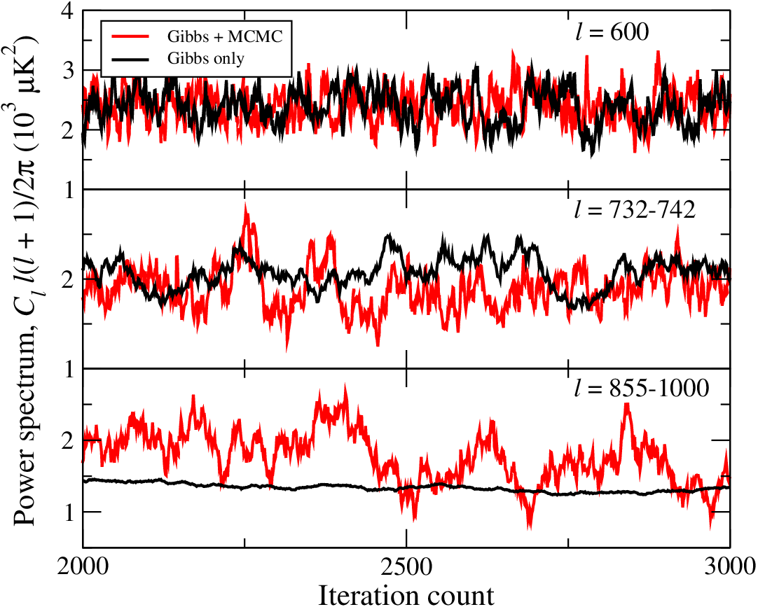
We first consider the full-sky data set, and in Figure 1 we show a segment of each of the two longer chains for three selected multipole bins. The top panel shows , which is the first bin to be sampled by MCMC, the middle panel shows , where there is still some signal in the data, and, finally, the bottom panel shows , which is strongly noise dominated. Starting with the top panel, we see that the red curve (Gibbs+MCMC) scatters significantly faster than the black curve (Gibbs only), implying more efficient sampling. This trend becomes even stronger with lower signal-to-noise, until the last case, where the Gibbs-only chain essentially does not move at all, while the MCMC sampler does probe the full range. Note, however, that even the MCMC sampler has a significant correlation length in this range, and this implies that there is still some room for improvement to be made in defining our proposals.
Next, these considerations are quantified in Figure 2, where we plot the Markov chain correlation length as a function of distance in the chain, for six bins with and without the MCMC sampler. As first reported by Eriksen et al. [4], we see that the Gibbs-only correlation length increases dramatically with decreasing signal-to-noise, rendering the algorithm essentially useless in this regime. However, we also see that the new MCMC step effectively resolves this issue, as the correlation length (here defined by having a correlation less than 0.2) now is less than steps. This is a dramatic improvement, and makes the algorithm useful even in this range. Nevertheless, we once again point out that it is possible to make further improvements by establishing better proposal densities.

In Figure 3 we consider the convergence properties of the k samples set, by computing the Gelman-Rubin statistic [10] as a function of . Typically, one recommends that should be less than, say, 1.2 in order to claim convergence. We see that this holds everywhere for this sample set, and typically it is even less than 1.05. Note also the step at , showing clearly the beneficial effect of the MCMC sampler.

Next, in Figure 4 we compare the marginal distributions derived from this sample set with the analytic result,
| (22) |
Here indicates a given multipole bin, denotes the product of the instrumental beam and the HEALPix pixel window, and is the power spectrum of the noisy data map. We see that the new algorithm reproduces the analytic distributions very well, and this verifies the overall method.

Finally, the cut-sky power spectrum with one-sigma confidence regions is shown in three panels in Figure 5, focusing on different -ranges, namely all ’s, the transition region, and the low region. This completes the high- temperature analysis validation.
IV.2. Polarization analysis
We now consider polarization analysis, and construct a new low- simulation for this purpose. This simulation does not mimic any planned experiment, but is rather designed to highlight the analysis method itself. Specifically, we drew a new CMB realization from the best-fit WMAP CDM spectrum that includes a non-zero tensor contribution, including multipoles up to , and convolved this with a FWHM Gaussian beam, and pixelized it at . Uniform noise of RMS was added to the temperature component, and RMS to the polarization components. The 5-year WMAP polarization sky mask was imposed on the data.
We allowed for non-zero , , and spectra, but fixed . These spectra were then individually binned to maintain a reasonable signal-to-noise per bin. (Details on how to introduce individual binning of each power spectrum were recently described by Eriksen and Wehus, 2008.) Again, a tuned Gaussian proposal density was used in the MCMC step. A total of 12 000 samples were produced over 12 chains, and the CPU time per sample was 55 seconds, for a total of CPU hours.

In Figure 6 we show one chain for each of the four sampled spectra, for the last (and therefore most difficult) bin in each case. Note that the and spectra have essentially vanishing signal-to-noise, and therefore these chains reach zero values. Clearly, we see that mixing properties of these chains are satisfactory, and the correlation lengths are quite short.

In Figure 7 we show the Gelman-Rubin statistics for each of the four power spectra, and with the single exception of the very last bin of , all values are well below 1.1. Thus, all spectra have converged well everywhere.

Finally, in Figure 8 we show the reconstructed marginal power spectra for each polarization component, overplotted on the input spectrum. The agreement is very good. Note, however, that these spectra are direct marginals, and not a joint maximum likelihood estimate. They are therefore not individual unbiased estimators. In particular, the marginal power spectrum is biased slightly high because of the combination of the positivity constraint and relatively low signal-to-noise. Consideration of the joint polarization posterior, which is an unbiased estimator, is postponed to a future publication.
V. Conclusions
We have presented a new MCMC algorithm for the high-L, low signal to noise limit of the joint posterior which solves the slow probabilistic convergence of the traditional Gibbs sampler in this regime. This in principle allows sampling over the joint posterior over the entire range of angular scales probed by current and future CMB experiments. The limiting computational burden is now entirely in the map-making step of Gibbs sampling, for which the cost per Gibbs iteration now scales with the expense of multiplication by the inverse noise matrix . Assuming pixel uncorrelated (but scan weighted) noise as a good approximation at small angular scales, the cost of an multiplcation is that of a forward and inverse spherical harmonic transform, or . Future work will attempt to push the generalized Gibbs + MCMC sampling scheme presented here to smaller angular scales, ultimately limited by the degree to which we can compute harmonic transforms.
Appendix A Including Deterministic Proposals in MCMC
Here we review the derivation of the accept probability in Markov Chain Monte Carlo when using deterministic proposals (or proposals where some of the degrees of freedom are specified as deterministic functions of the past state and/or proposed variations in some other degrees of freedom). We first briefly review the Metropolis-Hastings Markov Chain Monte Carlo algorithm and the proof of its convergence, and then turn to the special case involving deterministic proposals. Much of the review of the MCMC algorithm here follows [27]. We also note that similar technical considerations including deterministic elements in proposals are presented in [13] in the context of MCMC algorithms in which the dimension of the state space itself is included as a random variable to be sampled over.
The goal is the construction of a transition matrix such that after initializing the Markov Chain with a sample from any probability density , we generate samples from a sequence of probability densities
| (A1) |
which eventually converge to an equilibrium density
| (A2) |
We remind the reader of the sufficient conditions to establish convergence of an MCMC algorithm: stationarity, which means that the MCMC transition matrix satisfies
| (A3) |
and irreducability, which means that for any two states, there is a finite number of iterations which give a non-vanishing probability to transition from one state to the other. It is well known that these two properties are sufficient to establish convergence, as can be seen simply from the triangle inequality
The Metropolis-Hastings Markov Chain Monte Carlo algorithm is one method of constructing such a transition matrix. We choose any proposal matrix and then accept the proposed move with a probability
| (A4) |
while rejecting the proposed move with probability leads to a “null transition” where the next state in the Markov Chain remains the same. Application of this algorithm then leads to the sequence of probability densities which satisfy
| (A5) | |||||
where the first term is the constribution to the probability density if we reject any proposed move, while the second term is the contribution from accepting the proposed move from any possible previous state. If we demand that, for a chosen proposal matrix, the accept probability satisfies
| (A6) |
then we see that the MH MCMC algorithm satisfies stationarity, i.e. denoting by the density resulting from one application of the transition matrix to , we have directly from detailed balance
| (A7) | |||||
We now turn to the case where our proposal is of the form
| (A8) |
where we randomly propose a new power spectrum, posibly in a manner conditionally denpendent on the current spectrum and the data, and then deterministically compute a new CMB map with some function
| (A9) |
To satisfy detailed balance with a non-vanishing accept probability our function must satisfy
| (A10) |
or, that the inverse function is equivalent to interchanging the order of the power spectrum arguements
| (A11) |
In this paper, we have chosen one such function, given by
| (A12) |
where interchanging the spectra in the function above does in fact give the inverse function itself.
Our job now is to derive the accept probability such that we satisfy stationarity (as discussed above). For the proposal with deterministic changes to some of the degrees of freedom, stationarity is satisfied if
In order to determine the integral over the -function in the accept term above, we recall the identity for , where ,
| (A13) |
In our case, we can identify
| (A14) |
which vanishes at . We also have the Jacobian
| (A15) |
(i.e. is considered a function of with the other CMB map considered fixed) which therefore gives
| (A16) |
Inserting this into the condition for stationarity we have
where in the second line we again used the property that the inverse is equivalent to with the spectra arguements interchanged. We see from the above that a sufficient condition for stationarity is
| (A17) |
An accept probability which satisfies this condition therefore gives cancellation of the integrals over the -functions for both the reject and accept contributions, leaving us exactly with . We therefore have the accept probability
| (A18) |
We give the expression above for the general case of any deterministic change in the CMB map with a function which satisfies . We now explicitly evaluate this accept probability for the functional form chosen for this paper.
Since we have , we have
| (A19) |
Reminding the reader of the functional form of the joint posterior in eqn. 7, we have the accept probability given by
| (A20) | |||||
where the last line follows from the invariance of the quadratic form under the functional mapping . Finally, we note that for the special case of a symmmetric proposal matrix where , the accept probability is completely determined by the (exponeniated) change in
| (A21) |
As emphasized earlier in the main part of the text, the above allows large changes to the spectrum precisely where the signal to noise is getting small, as does not change much in this regime.
Appendix B Relation to Gibbs Sampling in a Change of Variables
We note here another interesting approach to an MCMC algorithm in a different set of variables which in fact allows for large moves in the spectrum in the low signal to noise regime. We define the CMB map
| (B1) |
We therefore have the joint posterior in the new variables according to
| (B2) |
which is explicitly, up to a normalization constant
| (B3) |
Then traditional Gibbs sampling in the new variables leads to an accept probability when changing the spectrum given the change of variable map as
| (B4) |
where in the above the proposed variation in the spectrum can now be conditionally dependent on the current change of variable map . Assuming a symmetric proposal, or one conditionally independent of leads to an accept probability which is numerically the same as A20 , and also has the same property - large moves in the spectrum are possible in the low signal to noise regime. As a side note, we can see that is quadratic in , and suggests a proposal given by a Gaussian in . However there are two problems with this scheme - sampling in will result in re-introducing a Jacobian factor given by the ratio of which results typically in low acceptance probabilities, and furthermore we cannot afford to exactly compute the local “Fisher” covariance matrix for each . Because of these difficulties, we in general need to produce a proposal for and then compute the accept probability above.
We emphasize an important distinction between MCMC with deterministic steps in the original variables and Gibbs sampling in the change of variables . It is only for the specific functional form that we have chosen for this paper that the numerical value of the accept probabilities for and are the same.
At first glance, it might appear that a random variation in some of the variables followed by a deterministic change in the complementary set is always equivalent to random variation in a new set of variables. For notational convenience, we will assume the state space is separated into two sets of variables , i.e. for the CMB sampling context we have . Now, to make the distinction between a change of variables and deterministic steps in MCMC more precise, consider a “global” change of variables of the form
| (B5) |
with Jacobian
| (B6) |
A Gibbs sampling step varying with fixed, has accept probability
where in the above we have the constraint
| (B8) |
Now consider an MCMC step in the original variables of the form
| (B9) |
with general accept probability, according to the discussion above
| (B10) |
Interestingly enough this suggests that we can set to be the function
| (B11) |
Does this function have the correct properties for its inverse? Assuming we have computed in the forward direction , we can invert to find by computing sequentially
| (B12) | |||||
where the last line follows from definition of the forward . Since we have, by definition
we therefore have shown that
| (B13) |
as required for a non-vanishing accept probability. The above as a function of has Jacobian
However, when evaluated at , we will not in general satisfy the required equality required for numerical equivalence
| (B15) |
So in general, while we can use any function to generate deterministic moves in the original variables within MCMC, this is not equivalent to a Gibbs sampling step in the new variables using as a global change of variables.
However, using the above construction for the CMB change of variables, we have explcitly
| (B16) |
which is exactly the functional form used for the deterministic MCMC steps. In this case, it is because the Jacobian of our deterministic change in the CMB map is independent of the current CMB map (and only dependent on the proposed and current spectra) that we have numerical equivalence of the accept probabilities.
So in summary, while we can use any mapping to generate deterministic steps for use in MCMC, the accept probability is not equivalent to a conditional step using in a change of variables due to the general “location” dependence of the Jacobian. Furthermore, setting is not the most general form for a function that satisfies the detailed balance requirement . In this sense then, a change of variables as an approach to more efficiently generating samples from a probability density is distinct from a strategy of designing an MCMC algorithm (in any chosen representation of the variables) with deterministic changes of some of the degrees of freedom. Both approaches are interesting, and advances in either approach for Bayesian CMB analysis could lead to improvements over the approach presented in this paper.
References
- [1] Abramowitz, M., & Stegun, I. A. 1972, Handbook of Mathematical Functions, New York: Dover, 1972,
- [2] Bennett, C. L., et al. 2003a, ApJS, 148, 1
- [3] Chu, M., Eriksen, H. K., Knox, L., Górski, K. M., Jewell, J. B., Larson, D. L., O’Dwyer, I. J., & Wandelt, B. D. 2005, Phys. Rev. D, 71, 103002
- [4] Eriksen, H. K., et al. 2004, ApJS, 155, 227
- [5] Eriksen, H. K., et al. 2007a, ApJ, 656, 641
- [6] Eriksen, H. K., Huey, G., Banday, A. J., Górski, K. M., Jewell, J. B., O’Dwyer, I. J., & Wandelt, B. D. 2007b, ApJ, 665, L1
- [7] Eriksen, H. K., Jewell, J. B., Dickinson, C., Banday, A. J., Górski, K. M., & Lawrence, C. R. 2008a, ApJ, 676, 10
- [8] Eriksen, H. K., Dickinson, C., Jewell, J. B., Banday, A. J., Górski, K. M., & Lawrence, C. R. 2008b, ApJ, 672, L87
- [9] Eriksen, H. K. & Wehus, I. K. 2008a, ApJS, submitted, [astro-ph/XXXXXX]
- [10] Gelman, A., & Rubin, D. 1992, Stat. Sci., 7, 457
- [11] Gold, B., et al. 2008, [arXiv:0803.0715]
- [12] Górski, K. M., Hivon, E., Banday, A. J., Wandelt, B. D., Hansen, F. K., Reinecke, M., & Bartelmann, M. 2005, ApJ, 622, 759
- [13] Green, P.; 1995, Biometrika, 82: 711-732
- [14] Gupta, A. K. & Nagar, D. K. 2000, Matrix Variate Distributions
- [15] Hinshaw, G., et al. 2007, ApJS, 170, 288
- [16] Hinshaw, G., et al. 2008, ApJ, submitted, [arXiv:0803.0732]
- [17] Hivon, E., Górski, K. M., Netterfield, C. B., Crill, B. P., Prunet, S., & Hansen, F. 2002, ApJ, 567, 2
- [18] Jewell, J., Levin, S., & Anderson, C. H. 2002, astro-ph 0209560v1
- [19] Jewell, J., Levin, S., & Anderson, C. H. 2004, ApJ, 609, 1
- [20] Komatsu, E., et al. 2008, [arXiv:0803.0547]
- [21] Larson, D. L., Eriksen, H. K., Wandelt, B. D., Górski, K. M., Huey, G., Jewell, J. B., & O’Dwyer, I. J. 2007, ApJ, 656, 653
- [22] Liu, J. S., Monte Carlo Strategies in Scientific Computing, Cambridge, USA: Springer, 2001,
- [23] O’Dwyer, I. J., et al. 2004, ApJ, 617, L99
- [24] Page, L., et al. 2007, ApJS, 170, 335
- [25] Seljak, U., & Zaldarriaga, M. 1996, ApJ, 469, 437
- [26] Smoot, G. F., et al. 1992, ApJ, 396, L1
- [27] Sokal, A.D.; “Monte Carlo methods in statistical mechanics: foundations and new algorithms”, Cous de Troisième Cycle de la Physique en Suisse Romande, Lausanne.
- [28] Taylor, J. F., Ashdown, M. A. J., & Hobson, M. P. 2007, MNRAS, submitted, [arXiv:0708.2989]
- [29] Wandelt, B. D., Larson, D. L., & Lakshminarayanan, A. 2004, Phys. Rev. D, 70, 083511
- [30] Zaldarriaga, M., & Seljak, U. 1997, Phys. Rev. D, 55, 1830