Neutrino Mixing and the Private Higgs

In the $\{h\phi_{1}\phi_{2}\}$ model, a charged scalar field $h^{+}$ is coupled to leptons according to

where $(i,j)$ and $(a,b)$ are $SU(2)$ and family indices respectively and Fermi statistics dictate that the coupling $f_{ab}$ is antisymmetric in $ab$. To obtain a Majorana neutrino mass we need an overall lepton number violation $\Delta L=2$. Therefore, (9) by itself does not generate a neutrino mass term since we can in principle assign $L=-2$ to $h^{+}$. In the original $\{h\phi_{1}\phi_{2}\}$ model, the desired lepton number violation was generated by coupling $h^{+}$ to two Higgs doublets $\phi_{1}$ and $\phi_{2}$.

Now the PH model enters into action. We have plenty of Higgs doublets around and we can promptly write down the cubic interaction originally proposed for the $\{h\phi_{1}\phi_{2}\}$ model

where the sum runs over all the fermions in the SM and ${\hat{M}}_{ff^{\prime}}$ is, due to Bose statistics, an antisymmetric “mass” coupling. Due to this antisymmetry, the $\{h\phi_{1}\phi_{2}\}$ model requires the presence of more than one Higgs doublet, as was noted in the original paper [11]. Within the PH scheme, we have plenty of Higgs doublets around for the $h^{+}$ field to couple to. However, the expression in (10) is not invariant under $K_{f}$ (for $f\neq e$), unless $f=f^{\prime}$ in which case the expression vanishes.

Lo and behold there is a readily available way out within our model! We have our scalar darkons so that we could promote the cubic coupling above to a dimension-4 operator. We are not quite there yet, since $h^{+}$ is invariant under all $K_{f}$, and the term

seems to be ruled out. Here is where our $\phi_{e}$ saved the day, since there is no $K_{e}$ and therefore the discrete symmetries $K_{\mu},K_{\tau},K^{s}_{e}$ and $K_{q}$ allow the quartic term

with $\rho_{f}$ some dimensionless coupling constants. Notice that the term $f=e$ vanishes so we do not have to worry about the piece having $S_{e}$.

The PHs and the darkons do not carry lepton number, and hence, had we chosen to charge $h^{+}$ with two units of lepton number, this term (12) would violate lepton number by two units. In other words, the clash between (12) and (9) generates neutrino masses at one loop as in Fig 1. We denote this model as $h$-PH.

Notice that, after the $\phi_{f}$’s pick up a vev, the terms in (12) produce $\rho_{t}v^{2}(\phi^{-}_{e}h^{+})$ (since the top PH vev dominates) and thus mix $\phi_{e}$ and $h$. Therefore, in principle we could have a tree level contribution from this term to $\mu\to e\nu\nu$. However, the new physics contribution is suppressed by a factor of $\rho_{t}\frac{v^{2}}{M_{h^{+}}^{2}}\frac{v^{2}}{M_{\phi_{e}}^{2}}\sim\frac{\rho_{t}m_{e}v}{\gamma_{te}M_{h+}^{2}}$ with respect to the SM decay via a $W$ boson. Since we expect $M_{h^{+}}>v$ the new physics contribution is negligible.

Other type of processes, such as those studied in [13], can be shown to be too small to be observed. For instance, The tree level contribution to neutrinoless double beta decay (see Fig (4a) in [13]) is suppressed by $\frac{\langle\phi^{0}_{e}\rangle v}{M_{\phi_{d}^{2}}}\sim\frac{m_{d}m_{e}}{v^{2}}\sim 10^{-10}$. Similarly with $\mu-e$ conversion in nuclei (see Fig (4b) in [13]).

Unfortunately the $h$-PH carries the seed of the simplest version of the $\{h\phi_{1}\phi_{2}\}$ model, which seems to be disfavored by experiment, since it favors the so called bi-maximal neutrino mixing matrix. In particular $V_{e2}$ comes out to be too large [16, 17, 18, 19, 20]. Therefore, we will now include the scalar singlet $k^{++}$ from the $\{hhk\}$ model.

In the original $\{hhk\}$ model [12] the Lagrangian is augmented by the following terms

where $\tilde{M}$ is a mass scale. A Majorana neutrino mass is generated at two loops as shown in Fig 2.

First of all, notice that in the PH model, in contrast to the original $\{hhk\}$ model, the coupling of $k^{++}$ to the charged leptons is now constrained by the $K_{\mu,\tau}$ symmetries to be diagonal, e.g. ${\tilde{f}}_{ab}={\tilde{f}}_{a}\delta_{ab}$.

Secondly, in the spirit of reducing the number of dimension 3 operators, we will introduce a real scalar singlet $\varphi$ blind to the SM gauge symmetries. We denote the model as $\varphi kh$-PH, and the Lagrangian reads

Contributions to the neutrino mass follow at two loops once the field $\varphi$ picks a vev, e.g. $\langle\varphi\rangle=v_{\varphi}$. The spontaneous breaking is driven by the potential $V(\varphi)$, which also depends on other fields. As an example, let us consider a $Z_{2}$ discrete lepton symmetry for $\varphi$ such as $\varphi\to e^{iq_{\varphi}\frac{\pi}{2}}\varphi$, with $q_{\varphi}=2$ (e.g. $\varphi\to-\varphi$). Therefore a natural way to introduce an instability in the $\varphi$ sector is via the terms

For the illustrative region of parameter space we considered (recall $\langle S_{f}\rangle\sim v$ for all fermions other than the electron) we will naturally generate $v_{\varphi}\sim v$, as well as an extra scalar particle around the same scale which will also contribute to the dark sector. In what follows we will study in more detail the $\varphi kh$-PH model, in particular the neutrino mass hierarchy and mixing.

Let us analyze in more detail the extra terms in the Lagrangian we needed to add in our $\varphi kh$-PH model, in particular regarding the symmetries of our theory. We started with three conserved lepton numbers in the charged lepton sector. To generate neutrino masses we needed to break lepton number by two units. We have then a choice regarding lepton charge for the extra fields, $h,k,\varphi$, to generate neutrino masses and a phenomenologically viable mixing pattern. In principle that can also introduce non-diagonal terms in the Yukawa sector and the undesirable FCNC and decays such as $\mu\to eee$, which are strongly bounded. We will come back to this point later on.

With this set up, radiative corrections generate the Majorana neutrino mass term $M_{ab}\nu_{L}^{a}C\nu_{L}^{b}$ with the symmetric matrix $M_{ab}$. Within our model, there is plenty of opportunities to allow various couplings and vacuum expectation values to be complex and thus violate CP. We will not discuss CP violation here and will thus take $M_{ab}$ to be real, purely for the sake of simplicity.

As mentioned earlier, we pursue here a natural approach of preserving $L_{e}$ as a symmetry to first approximation. In a sense we replace $K_{e}$ by $L_{e}$. We thus assign $L_{(e,\mu,\tau)}=0$ to $h^{+}$. Hence to ensure $L_{e}$ is conserved we are led to impose $f_{e\mu}=0$ and $f_{e\tau}=0$. We also enforce ${\tilde{f}}_{e}=0$ by having both $\varphi$ and $k^{++}$ invariant under $L_{e}$.

Notice that the symmetries we imposed imply $M_{ee}=0,M_{e\mu}=0,M_{e\tau}=0$, but $M_{\mu\tau}\neq 0,M_{\mu\mu}\neq 0,M_{\tau\tau}\neq 0$, which leads to the normal hierarchy with $m_{1,2}\sim 0\ll m_{3}$. As we will see, a very interesting pattern appears from our assumptions.

The $f_{\mu\tau}$ coupling leaves conserved ${\tilde{L}}=L_{\mu}-L_{\tau}$ as alluded to earlier. However, lepton number is explicitly broken by the $\varphi kh$ sector. Since $k^{++}$ is lepton-blind, the couplings to the right handed scalar $l^{a}_{R}l^{a}_{R}$ also break ${\tilde{L}}$ softly. Nevertheless, notice that before symmetry breaking we can assign lepton number charges such that $L_{e},L_{\tau},L_{\mu}$ are conserved, for instance by setting ${\tilde{f}}_{\tau}=0$, as well as $L_{\mu}=+2$ and $-2$, for $k^{++}$ and $\varphi$ respectively. In this scenario the $\varphi kh$-PH Lagrangian preserves $L_{e}$ and $\tilde{L}$. That is enough to guarantee that FCNC are not generated before $\varphi$ picks a vev and $\tilde{L}$ is softly broken by the introduction of ${\tilde{f}}_{\tau}\neq 0$. On the other hand, Flavor Changing Charged Currents (FCCC) could be present in the $\mu-\tau$ sector like those induced from the $f_{\mu\tau}$ coupling itself. In what follows we will ignore FCCC and FCNC, we will show later on these are highly suppressed.

So far so good, our theory posses a $L_{e}$ symmetry and neutrino masses are radiatively induced with $M_{eb}=0$ for $b=e,\mu,\tau$. In principle we can make do with a neutrino mass matrix with texture $M_{eb}=0$. However, to better fit the experimental data we will relax $L_{e}$ and allow for a small soft breaking, but first let us get a glimpse of the order of magnitude for the entries in the neutrino mass matrix, which as we shall see are generated by different mechanisms.

In general in the original $\{h\phi_{1}\phi_{2}\}$ model, even though neutrino masses are radiatively induced, we still had to consider a very small $f_{ab}$, of the order of $10^{-5}-10^{-6}$ in (9), in order to produce values of $10^{-2}$ eV for neutrino masses. That is however not the case in the $\varphi kh$-PH model. At one loop $k^{++}$ does not enter and ${\tilde{L}}=L_{\mu}-L_{\tau}$ conservation implies that the only non-zero entry in the mass matrix is $M_{\tau\mu}$, from the $h$-PH piece in the Lagrangian. The diagram in Fig 1 with the $\tau$ in the loop (the same diagram with $\mu$ in the loop is down) gives

where we have introduced the reduced coupling

assuming $M_{\phi_{\tau}}>M_{h^{+}}$. We next use (see (36)) $M_{\phi_{\tau}}^{2}=\gamma_{t\tau}\frac{v}{\sqrt{2}}\frac{v^{t}_{s}v^{\tau}_{s}}{2\langle\phi^{0}_{\tau}\rangle}$ with $v^{\tau}_{s}\equiv\sqrt{2}\langle S_{\tau}\rangle$. As explained in the Appendix we assume $v^{\tau}_{s}\sim v^{t}_{s}\sim v\sim 246$ GeV. Setting $y^{PH}_{\tau}\sim y^{PH}_{e}\sim 1$ in $m_{\tau}\sim y^{PH}_{\tau}\langle\phi^{0}_{\tau}\rangle$ and $m_{e}\sim y^{PH}_{e}\langle\phi^{0}_{e}\rangle$, we obtain

A crude estimate (assuming ${\rho_{\tau}\sim\gamma_{t\tau}}$) sets the neutrino mass scale around

which naturally falls in the $10^{-2}-10^{-3}\mbox{eV}$ range with $f_{\mu\tau}\sim 10^{-1}-10^{-2}$, a much more reasonable value than the value mentioned above. The range of course depends on our various other “reasonable” values of the other couplings in the theory.

At this point, the neutrino mass matrix takes the form

which obviously falls short in accounting for data. The next step is to fill up the diagonal entries. Recall $L_{e}$ is still conserved. Thus at two loops (see Fig 2) the $k^{++}$ part of our Lagrangian will generate non-zero values only for $M_{\mu\mu}$ and $M_{\tau\tau}$. Interestingly, these two-loop contributions could compete with $M_{\tau\mu}$. In fact, we get (assuming $M_{k^{++}}$ larger than $M_{h^{+}}$)

where the reduced coupling ${f^{\prime}}_{\mu\tau}$ here is defined with the logarithmic factor Log$\left({M_{k^{++}}\over M_{h^{+}}}\right)$ rather than the factor in (17). We will simply assume that these logarithmic factors are comparable for the sake of argument and thus obtain (for $v_{\varphi}\sim v$)

Even though we have a $\frac{v}{m_{e}}$ enhancement, $M_{\mu\mu}$ is suppressed by ${\tilde{f}}_{\tau}{f^{\prime}}_{\mu\tau}\sim{\tilde{f}}_{\tau}\times(10^{-3}-10^{-4})$. Since $m_{e}\sim 10^{-6}v$ finally we get

which can be made comparable for $M_{k^{++}}\sim\sqrt{\tilde{f}_{\tau}}10v\sim$ TeV scale, but keep in mind that there are many other parameters which could change our crude estimate.

We next turn to $M_{\tau\tau}$, generated by the diagram that produces $M_{\mu\mu}$ but with the muon in the internal line rather than the $\tau$. Thus we obtain

which seems to favor a much smaller $M_{\tau\tau}$. Here we have two choices. We could either take ${\tilde{f}}_{\mu}\sim{\tilde{f}}_{\tau}$ and hence $M_{\tau\tau}<<M_{\mu\mu}\sim M_{\mu\tau}$, or take $M_{\tau\tau}\sim M_{\mu\mu}\sim M_{\mu\tau}$, arguing that all three of these entries in the neutrino mass matrix are quantities of the same type, in contrast to quantities associated with the electron family. With various couplings around we could readily achieve this by taking ${\tilde{f}}_{\tau}\sim{\tilde{f}}_{\mu}\frac{m_{\mu}^{2}}{m_{\tau}^{2}}\sim f_{\mu\tau}$ somewhat smaller and ${\tilde{f}}_{\mu}\sim 1$ somewhat larger. In fact, as we discussed before, ${\tilde{f}}_{\tau}$ is responsible for the soft breaking of ${\tilde{L}}$ and therefore it could be naturally smaller than ${\tilde{f}}_{\mu}$. In that case, we lower the mass scale for $k^{++}$ and it could be around the corner.

Of course these are rough estimates which merely serve to motivate us to “predict” a form for the neutrino mass matrix. So far, we have filled up the lower right corner, so that

with $x\sim y$ and either $z\sim y$ or $z\ll y$. Now our mass matrix is closer to reproduce observations.

Let us remark that our model has the virtue of having very little fine tuning of dimensionless constant. Indeed, the only hierarchy we stumble upon is $f_{\mu\tau}\sim 10^{-1}-10^{-2}$, which is a small price to pay to accommodate all observed fermion masses and mixing in a compelling framework (Note in passing that $f_{\mu\tau}\sim\lambda^{2}-\lambda^{3}$, with $\lambda\sim 0.2$ from the CKM mixing.). In addition, if we take $M_{\tau\tau}\sim M_{\mu\mu}$ (that is, $y\sim z$) we would also need ${\tilde{f}}_{\tau}\sim{\tilde{f}}_{\mu}\frac{m_{\mu}^{2}}{m_{\tau}^{2}}\sim f_{\mu\tau}\sim 10^{-2}{\tilde{f}}_{\mu}$.

The final step down the road is to allow for small (soft) violations of $L_{e}$ to lift the zeros in our matrix up to non-zero but small values. In other words, we introduce a non-zero $f_{eb}$ such that $|f_{eb}|<|f_{\mu\tau}|$ for $b=\mu,\tau$. We also have to worry about FCNC, specially in the electron sector due to small violations of $L_{e}$, for instance in processes such as $\mu\to eee$. However, the process $\mu\to eee$ is highly suppressed since the mass of the neutrino appears explicitly in the one-loop (see Fig. 3) generated coupling of $\phi^{0}_{e}$ to $\mu e$, giving a branching ratio of order

where ${{\hat{f}}}_{e\mu}$ is defined similarly as in (17) with $\tau\leftrightarrow\mu$, and we considered $f_{e\mu}\sim 0.1f_{\mu\tau}\sim 10^{-2}-10^{-3}$, for which the rate is totally unobservable. Similarly for $\tau\to eee$ and other FCNC processes. For instance, the decay $\mu\to e\gamma$ is equally suppressed. The decay is described by a diagram similar to the diagram in Fig. 3 with $\phi^{0}_{e}$ replaced by its vev and a photon emitted from the $h^{+}$ loop.

For the case of FCCC similar considerations apply. For instance, we can generate the coupling $\phi_{\mu}e\bar{\nu}_{e}$, that will contribute to the dominant SM muon decay channel. The contribution is already loop suppressed ($\sim{\hat{f}}_{e\mu}$), and in addition we have $\frac{M_{W}^{2}}{M_{\phi_{\mu}}^{2}}\sim\frac{m_{\mu}}{v}\sim 4\times 10^{-4}$. Therefore, the correction is negligible. In principle we could also have FCCC induced by FCNC. For instance, a diagram similar to Fig. 3 generates a coupling of $\phi_{\mu}^{0}$ with $\mu e$ which in turn induces an effective coupling of the sort $\phi^{+}_{e}\mu^{-}\bar{\nu}_{\mu}$. Henceforth we can get contributions to $\mu^{-}\to\bar{\nu}_{\mu}e^{-}v_{e}$ which are experimentally constrained. However, as we have seen so far, in the PH model it follows that these effects are strongly suppressed given the high scale of the PHs, or in other words the lightness of the charged leptons involved, which renders these decays unobservable.

Adding $f_{eb}$ into the game we end up with the following texture for the neutrino mass matrix

with $m_{\nu}\sim 10^{-2}$ eV setting the neutrino scale. Here $M_{ee}$ arises from two-loop diagrams similar to Fig 2 and it is therefore suppressed by $\delta^{2}$ with respect to $M_{\mu\mu}$, with $\delta\sim\frac{f_{e\tau}}{f_{\mu\tau}}$.

On the other hand, $M_{e\mu}$ and $M_{e\tau}$ are generated in one-loop order by diagrams similar to that shown in Fig 1. Here the peculiar structure of the quartic coupling in (12) gives rise to an interesting structure. The PH field $\phi_{e}$ associated with the electron could be either disappearing into the vacuum or circulating in the loop. In the second possibility, the largest contribution comes from $\phi_{t}$ (the SM Higgs) disappearing into the vacuum. We denote the two contributions respectively as $M_{e\mu}=M_{e\mu}^{(e)}+M_{e\mu}^{(t)}$ and similarly for $M_{e\tau}$. Note that for $M_{\mu\tau}$ the only possibility is for $\phi_{e}$ to go into the vacuum. We have $M_{e\mu}^{(e)}\sim\rho_{\mu}v{\hat{f}}_{e\mu}m_{e}m_{\mu}\frac{1}{M_{\phi_{\mu}}^{2}}\sim\frac{\rho_{\mu}}{\gamma_{t\mu}v^{2}}{\hat{f}}_{e\mu}m_{e}m_{\mu}^{2}$. Similarly, $M_{e\mu}^{(t)}\sim{\rho_{t}\over\gamma_{te}v^{2}}{\hat{f}}_{e\mu}m_{t}m^{2}_{e}$ (compare with (18)). Thus

If we take the $\rho$’s and $\gamma$’s to be comparable for lack of knowing any better, we have $M_{e\mu}\sim M_{e\mu}^{(t)}$. On the other hand, again taking the $\rho$’s and $\gamma$’s to be comparable, we have $\frac{M_{e\tau}^{(t)}}{M_{e\tau}^{(e)}}\sim{\frac{m_{e}}{m_{\tau}}}{\frac{m_{t}}{m_{\tau}}}\sim{\frac{1}{30}}$ and so in this case the $``(e)"$ diagram rather than the $``(t)"$ diagram dominates, giving $M_{e\tau}\sim{M_{e\tau}^{(e)}}$. We conclude that

which suggests that $M_{e\mu}$ maybe somewhat smaller than $M_{e\tau}$, but since we don’t know the value of the ratio ${\frac{{\hat{f}}_{e\mu}}{{\hat{f}}_{e\tau}}}$ and of the ratios of the $\rho$’s and $\gamma$’s, not to mention ratios like $\frac{v^{s}_{t}}{v^{s}_{e}}$, $M_{e\mu}$ and $M_{e\tau}$ could easily be comparable. Therefore, in our phenomenological fits below, we generally take $M_{e\mu}$ to be somewhat smaller than or comparable to $M_{e\tau}$.

A very illuminating example follows from considering the following mass matrix

which complies with our theoretical bias. Notice that we take $M_{ee}$ and $M_{\tau\tau}$ to be negligible. From this simple matrix the mass ratio, $r$, comes out to be right on the money, $r=\frac{3-2\sqrt{2}}{4\sqrt{2}}+{\cal O}(\delta^{2})\sim\frac{1}{33}$. In particular we also have $m_{1}=0$. Unfortunately the mixing matrix fits data only partially. The value $\delta\sim\frac{1}{5}$ seems favored and we obtain

which has a very attractive $V_{e3}\sim 0.2$ but it is rather off in the lower right corner. Even though we should not rule it out, it seems disfavored.

As a second illustrative example, a very attractive fit emerges from the choice $\delta\sim\frac{1}{5}$, but $a\sim b\sim 1,~y\sim 1,~x\sim-1$, and $z\sim\frac{3}{5}$. The latter requires a hierarchy of the sort $\frac{{\tilde{f}}_{\mu}}{{\tilde{f}}_{\tau}}\sim 10^{2}$. The mass matrix reads

which leads to the mixing matrix

and a mass ratio $r=\frac{1901+51\sqrt{1601}}{51\sqrt{1601}-1901}\sim 0.03$. In addition, we also have for the mass eigenvalues $\frac{m_{3}}{m_{1}}=\frac{\sqrt{1601}+51}{51-\sqrt{1601}}\sim 8.3,~\frac{m_{2}}{m_{1}}=-\frac{20}{51-\sqrt{1601}}\sim-1.8$. Notice we have a small but non-zero $V_{e3}\sim 0.02$. Future experiments may be able to measure $V_{e3}$ down to a value $\sim 0.01$ [23]. All the matrix elements above are within the experimental bounds [21, 22].

While our model does not predict the matrix $M$ given here, we might optimistically hope that a group theoretic approach or a deeper theory (perhaps string theory) would one day produce this type of matrix.

A suggestive mixing matrix is the so called Tri-bimaximal matrix [24]

which can be approximately obtained in our model with a neutrino mass matrix with $\delta=\frac{1}{5}$, $a=1$, $b=1$, $y=0.9$, $x=-1.05$, $z=0.9$. That is

where again we tuned $z\sim y$. The tri-bimaximal mixing is very appealing, however, in our model the mass ratio comes out a bit too small, e.g. $r\sim 0.018$.

The three examples we illustrated above have different features. However our model seems to suggest a non-zero $V_{e3}$. Very nice fits emerge from the following mass matrices, $M_{A}$ and $M_{B}$.

where we used $\delta=0.1$, $a=1/2$, $b=3$, $x=-1.15$, $z=1$, $y=0.85$. The mass ratio comes out to be $r\sim\frac{1}{32}$, and the mixing matrix

and

where we used $\delta^{2}=0.02$, $a\delta=-0.06$, $b\delta=-0.35$, $x=1.3$, $z=-1.1$, $y=-1$. The mass ratio is $r\sim\frac{1}{30}$, and the mixing matrix

In both scenario we require some tuning of $M_{\tau\tau}$ to comparable values of $M_{\mu\mu}$. However we obtain a very appealing $V_{e3}\sim 0.09$ and within the observed values for $r$.

Notice that given the observed mixing matrix and mass squared differences, we could also simply apply linear algebra and “reverse engineer” [25, 26] to obtain the neutrino mass matrix in terms of one unknown parameter.

Notice that in our model we have $\frac{M_{ee}}{m_{\nu}}\sim\delta^{2}\ll 1$ which naturally suppresses neutrinoless double beta decay. In addition, from the algebraic relation

we have

Recall $r=\frac{\Delta m^{2}_{21}}{\Delta m_{32}^{2}}$. If we now define $p=\frac{m_{2}}{m_{3}},~q=\frac{m_{1}}{m_{3}}$ we have $r=\frac{p^{2}-q^{2}}{1-p^{2}}$. Within the normal mass hierarchy, $m_{1}<m_{2}\ll m_{3}$, hence $q^{2}<p^{2}\ll 1$, also $p<0$. Moreover, we can solve for $p(q,r)$ and plug it back in (29) to obtain

Biased by experiments we would like the ratio $r$ to stay within values $r\sim 0.03$, therefore we re-write $V_{e3}$ as

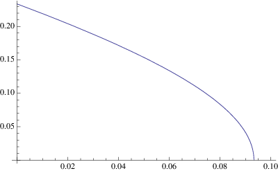
Let us explore the region of parameter space where we can ignore the factor of ${M_{ee}\over m_{3}}\sim\delta^{2}\ll 1$. Those are the cases where we expect a large contribution to $V_{e3}$ from the other terms. We can have an idea of the values we would expect by maximizing (31) using the smaller and larger experimental values for $V_{e1}$ and $V_{e2}$ respectively (see $|V^{3\sigma}_{exp}|$ [21, 22]). By taking $V_{e1}\sim 0.77$ and $V_{e2}\sim 0.63$ we notice that for values $0.05<q<0.15$ we have $0.05<|V_{e3}|<0.2$. Whereas on the other extreme end, with $V_{e1}\sim 0.86$ and $V_{e2}\sim 0.50$ we have $0.09<|V_{e3}|<0.2$ for values $0<q<0.05$. Finally we can plot (31) for the central values $V_{e2}=0.565$ and $V_{e1}=0.815$, for which we have (see plot in Fig 4.)

Amusingly we have $V_{e3}\to 0.23$ when $q\to 0$ and $V_{e3}\to 0$ as $q$ approaches $\sim 0.1$.

References

- [1] R.A. Porto and A. Zee, “The Private Higgs”, arXiv:0712.0448.
- [2] X-G. He, H-C. Tsai, T. Li, and X-Q. Li, Mod. Phys. Lett. A22, 2121 (2007).
- [3] V. Silveira and A. Zee, Phys. Lett. B 161, 136 (1985).
- [4] D. E. Holz and A. Zee, Phys. Lett. B 517, 239 (2001).
- [5] C. P. Burgess, M. Pospelov and T. ter Veldhuis, Nucl. Phys. B 619, 709 (2001).
- [6] B. Patt and F. Wilczek, arXiv:hep-ph/0605188.
- [7] O. Bertolami, R. Rosenfeld, arXiv:0708.1784.
- [8] C. Jackson, “ Dark Matter in the Private Higgs Model”, arXiv:0804.3792.
- [9] I. Gil-Botella, arXiv:0710.4258.
- [10] Daya Bay Collaboration, http://arxiv.org/abs/hep-ex/0701029.
- [11] A. Zee, Phys. Lett. 93B, 389 (1980).
- [12] A. Zee, Phys. Lett. 161B, 141 (1985), Nucl. Phys. B264 99 (1986).
- [13] For a review, see D. Chang and A. Zee, Phys. Rev D 61, 071303, (2000).
- [14] K.S. Babu, Phys. Lett. B203, 132 (1988).
- [15] M. Nebot, J. F. Oliver, D. Palao, and A. Santamaria, “Prospects for the Zee-Babu Model at the LHC and low energy experiments,” arXiv:0711.0483v2.
- [16] C. Jarlskog, M. Matsuda, S. Skadhauge, and M. Tanimoto, Phys. Lett. B449 (1999) 240, hep-ph/0005147.
- [17] P. H. Frampton and S. L. Glashow, Phys. Lett. B461 95 (1999).
- [18] Y. Koide, Phys. Rev. D 64 077301 (2001).
- [19] N. Haba, K. Hamaguchi, and T. Suzuki, Phys.Lett. B519, 243 (2001).
- [20] X-G. He, Eur.Phys.J. C34 (2004) 371-376
- [21] Concha Gonzalez-Garcia, http://www.dpf2003.org/xx/neutrino/concha.pdf.
- [22] Renata Zukanovitch Funchal, http://www2.phys.canterbury.ac.nz/ jaa53/presentations
- [23] John Learned. Private Communication.
- [24] P. F. Harrison, D.H. Perkins and W.G. Scott, Phys. Lett. B 530, 167 (2002); X. G. He and A. Zee, Phys. Lett. B560, 87(2003) hep-ph/0301092. L. Wolfenstein, Phys. Rev. D18, 958 (1978). P.F. Harrison, D. H. Perkins and W.G. Scott, Phys. Lett. B458, 79 (1999); W.G. Scott, Nucl. Phys. Proc. Suppl. 85, 177(2000); P. F. Harrison and W.G. Scott, Phys. Lett. B535, 163(2002); P.F. Harrison and W.G. Scott, Phys.Lett. B557 76 (2003), Z.-Z. Xing, Phys. Lett. B533, 85 (2002), C. I. Low and R. R. Volkas, Phys.Rev. D 68 033007 (2003).
- [25] A. Zee, hep-ph/0307155, in “Neutrinos, Flavor Physics, and Precision Cosmology” ed. J. F. Nieves and R. R. Volkas, page 74, 2003.
- [26] A. Zee, hep-ph/0307323, Phys.Rev. D68 (2003) 093002.