Central exclusive production of dijets
at
hadronic colliders
J.R. Cudella,11
1
jr.cudell@ulg.ac.be, A.
Dechambrea,22
2
alice.dechambre@ulg.ac.be, O. F.
Hernández,b,33
3
oscarh@physics.mcgill.ca ; permanent
address: Marianopolis College, 4873 Westmount Ave.,
Montréal, QC, Canada H3Y 1X9
I. P. Ivanova,c,44
4
igor.ivanov@ulg.ac.be
a IFPA, Département AGO, Université de Liège, Sart Tilman, 4000 Liège, Belgium
b Physics Dept., McGill University, 3600 University St., Montréal, Québec, Canada, H3A2T8
cSobolev Institute of Mathematics, Koptyug avenue 4, 630090, Novosibirsk, Russia
(August 24, 2026)
Abstract
In view of the recent diffractive dijet data from CDF run II, we critically re-evaluate the standard approach to the calculation of central production of dijets in quasi-elastic hadronic collisions. We find that the process is dominated by the non-perturbative region, and that even perturbative ingredients, such as the Sudakov form factor, are not under theoretical control. Comparison with data allows us to fix some of the uncertainties. Although we focus on dijets, our arguments apply to other high-mass central systems, such as the Higgs boson.
Introduction
The CDF collaboration has recently published the measurement of the cross section for exclusive dijet production [1]. These are important data, as the dijet system reaches masses of the order of 130 GeV, i.e. the region of mass where the Higgs boson is expected. Given the high centre-of-mass energy involved, , the process is entirely due to pomeron exchange. Thus the dijets are produced by the same physical mechanism which could produce the Higgs boson and other rare particles. The CDF data provide a good opportunity to tune the calculations of quasi-elastic diffractive processes which, as we shall show, are otherwise plagued with severe uncertainties.
Almost twenty years ago, Schäfer, Nachtmann and Schöpf [2] proposed the use of diffractive hadron-hadron collisions, where a high-mass central system is produced, as a way of producing the Higgs boson. Bjorken recognised such quasi-elastic reactions, in which the protons do not break despite the appearance of the high-mass system, as a “superb” channel to produce exotic particles [3]. The first evaluation was done in the Higgs case by Bialas and Landshoff [4]. It relied heavily on the use of non-perturbative propagators for the gluons, which provide an automatic cut-off of the infrared region. That calculation was then repeated by two of us [5], where we showed that by properly treating the proton form factors, one could use either perturbative or non-perturbative propagators. However, even with the use of form factors screening the long wavelengths of the exchanged gluons, one remained sensitive to the infrared region, as the gluons had a typical off-shellness of the order of 1 GeV. Berera and Collins [6] then calculated the double-pomeron jet cross sections using a perturbative QCD framework. They identified large absorptive corrections — corresponding to the “gap survival probability”, i.e. to multiple pomeron exchanges — as well as large virtual corrections — coming from the large difference of scales at the jet vertex, and resulting in a “Sudakov form factor”. However, they did not model these corrections.
Since then the subject of diffractive dijet and Higgs production has been extensively discussed from a variety of points of view [7]– [18]. All the calculations essentially follow the same pattern; the variations come in the following four ingredients:
- 1.
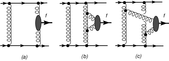
The two jets are at low rapidity, and at high transverse energy . They then come dominantly from gluon production at large transverse momentum (which we shall note ) and the partonic amplitude can be calculated in perturbative QCD. Furthermore, the two outgoing gluons are constrained to be in a colour-singlet state, and, to prevent colour flow in the channel, an extra screening gluon is exchanged (Fig. 1.a). The exact relation between the parton and the jet will be discussed in Section 6.2.
- 2.
As the gluons go from low transverse momenta in the proton to high ones in the jet system, there are enhanced double logarithms from vertex corrections (Fig. 1.b), which must be resummed to give the Sudakov form factor.
- 3.
- 4.

In this paper we want to evaluate, in view of the CDF data, the uncertainties in the various ingredients of the calculation of central exclusive dijet production. As discussed above, ours is not the first such calculation, however we believe to shed light on several important points. We show that the calculation still lies mostly in the non-perturbative region, and that many standard approximations cannot be justified. In particular, we find the following:
- •
At the Born level, exact transverse kinematics is important. That is to say, the momentum transfers to the hadrons cannot be neglected with respect to the momentum of the screening gluon, which makes the exchange colour-neutral. In Section 1, we present a detailed account of the part of the calculation which is under control, i.e. lowest-order via a colour-singlet exchange. There we take the exact transverse kinematics into account. Furthermore, diagrams in which the screening gluon participates in the hard sub-process cannot necessarily be neglected, as has been assumed in previous works. In Section 2.3, we show they could be important once the Sudakov suppression is taken into account. These issues affect the calculation of the partonic amplitudes mentioned above in ingredient 1.
- •
The leading and subleading logs that are resummed to give the Sudakov form factors are not dominant for the momentum range of the data, i.e. the constant terms are numerically important. This affects the calculation of double logarithm vertex corrections mentioned above in ingredient 2. We discuss the Sudakov form factor and the problems associated with the large virtual corrections in Section 2.
- •
The colour neutrality of the protons has to be implemented independently of the Sudakov suppression. This affects the calculations [8] that make use only of the Sudakov form factor to regulate the infrared divergences of the gluon propagators mentioned in ingredient 3. This is discussed in Section 3, where we consider various ways to embed the perturbative calculation into a proton.
In addition to these points, there remains the issue of gap survival, ingredient 4 in the list above. Providing an accurate numerical estimate of this is beyond the scope of this paper but we do discuss the gap survival probability and current estimates in Section 4.
In view of the above uncertainties, we try to outline a few scenarios that do reproduce the dijet data, and that can be extended to Higgs production at the LHC. After a few extra corrections, we give in Section 5 a simple estimate of the cross section, followed in Section 6 by detailed numerical results. Finally in Section 7 we present our conclusions.
1 The lowest-order perturbative QCD calculation
1.1 Kinematics

The backbone of the central quasi-elastic production of two high- jets is the partonic subprocess , in which the produced colour-singlet two-gluon system is separated by large rapidity gaps from the two scattering quarks. The kinematic conventions are shown in Fig. 2. We assume that the quarks are massless and consider the collision in a frame where the incoming quarks have no transverse momenta. Their momenta and , with , will be used as the lightcone vectors for the Sudakov decomposition of all other momenta entering the calculation. The momentum transfer to the first and second quarks are and , respectively, and are dominated by their transverse parts and (we write all transverse vectors in bold). The momenta of the two produced gluons are
| (1) |
The largest contribution to the cross section will come from the region where longitudinal components obey
| (2) |
as the invariant mass squared of the two-gluon system
| (3) |
is much smaller than . The differential cross section can then be written as a convolution over a phase space factorised between light-cone and transverse degrees of freedom:
| (4) |
The longitudinal phase space can alternatively be written as
| (5) |
If the two gluons are both integrated in the whole available phase space, then an extra should be put in the expression of the cross section due to Bose statistics.
1.2 Simplifications for the imaginary part
As we shall see, the lowest-order calculation will lead to an amplitude which grows linearly with . As the exchange is , the amplitude is then mostly imaginary, and can be calculated via their standard cuts. At the same lowest order, the real part is suppressed by a power of , however it will be only logarithmically suppressed at higher orders. In principle, it can be obtained via dispersion relations, but we do not concern ourselves with its contribution, as it will be much smaller than the large uncertainties in the other parts of the calculation.
In contrast to central Higgs production, two gluons can be emitted from all parts of the diagrams in many different ways, which is represented by the grey circle of Fig. 2. However, if one calculates the imaginary part of the amplitude, then there are multitudinous cancellations among different contributions due to the positive signature and colour-singlet nature of the exchange, as well as to the presence of large rapidity gaps. We show in Fig. 3 two typical cut diagrams that give rise to an imaginary part for jet production. The dashed line represents the kinematic cut of the diagram, i.e. it indicates which propagators are put on shell in the loop integral. The contributions of the “wrong cut” such as, for example, those shown in Fig. 3.b cancel one another. This means that one can write the amplitude as a sequence of two sub-amplitudes, gauge invariant on their own: , as in Fig. 3.a. Since in our case , there are three generic situations: (), (), or ().

Each of the sub-amplitudes in Fig. 3.a describes the emission of one or two gluons in the central region. In principle, all the vertices needed for the calculation of two-gluon production in arbitrary kinematics can be found in the literature. Production of one gluon can be described by the standard Lipatov vertex [21], while emission of two gluons involves an effective four-gluon vertex in the quasi-multi-Regge kinematics [22]. Such non-local vertices take into account gluon emission not only from the -channel gluons themselves, but also from the quarks. In the case of large transverse momentum of the produced gluons, which is the focus of the present paper, the situation simplifies, since emission from -channel gluons is dominant, and the amplitude is more conveniently calculated using Feynman diagrams and cutting rules.
1.3 Central production of two gluons with large transverse momentum
We are interested in the quasi-elastic production of two gluons with large relative transverse momenta of the order of tens of GeV. The requirement that the protons remain intact effectively cuts the differential cross section at small values of momentum transfers, , where is a typical proton elastic slope in hadronic reactions (for more discussion on what numerical value for would be most appropriate in our case, see Section 3.3). Therefore, , and the process can be viewed as a collision of two nearly-collinear but energetic gluons55 5 Strictly speaking, in the lab frame, one of these two gluons can be very soft and emitted at large angle relative to the quark collision axis. However, after an appropriate longitudinal boost the above description will become true. accompanied by an additional exchange of an extra screening gluon to restore the neutrality of the -channel colour exchange. The set of diagrams to be considered is then reduced to those of Fig. 4, and to their counterparts where each gluon is emitted from the other side of the cut.

Lowest-order diagrams with gluons emitted from different -channel gluons, such as the one of Fig. 4.b, are suppressed66 6 Note that the presence of hard transverse momentum in the -channel partons in these diagrams changes nothing since these partons are on-shell, so that the transverse momentum does not suppress the amplitude. by one extra power of . The situation may become different at higher orders, as we shall explain in Section 2.3. Also, as we are calculating cut diagrams, the sub-amplitudes are at the tree level and there are no ghost contributions.
The Mandelstam invariants in the two-gluon collision can be written
| (6) |
Note that these invariants depend only on the ratio , which is related to the difference of the rapidities of two produced gluons.
Let us also introduce the momenta of the colliding gluons
| (7) |
The imaginary part of the amplitude can be represented as
| (8) |
where
| (9) |
are the amplitudes with gluon polarisation vectors discussed below. Strictly speaking, the two colliding gluons are virtual. In our kinematics, their off-shellnesses are and , which are much smaller than . Since the hard scale of the scattering sub-process is given by , one can neglect the non-zero virtualities and approximate the amplitude by scattering of on-shell transversely polarised gluons, and neglect the contribution from the longitudinal polarisations. The calculation is then manifestly gauge invariant.
The helicity amplitudes for the tree-level scattering of two gluons in a colour-singlet state are most easily calculated in the centre-of-mass frame:
| (10) |
where is the azimuthal angle of the two-gluon-production plane with respect to the quantisation axis. Note that this quantisation axis is arbitrary, and changing it will produce changes in which will be compensated by opposite changes in .
The fact that Eq. (10) is written in a frame which is different from the laboratory frame does not pose any problem. Indeed, in order to pass from the laboratory frame to the centre-of-mass frame with gluons colliding along the axis, one first has to perform a longitudinal boost to make the energies of the colliding gluons equal, then a transverse boost to make the total momentum of two gluons zero, and then rotate the frame to align the axis with the direction of the incoming gluons. The large longitudinal boost does not change , while the transverse boost and the rotation by a small angle have negligible effect on the hard momentum . Therefore, one can safely understand in Eq. (10) as the azimuthal angle in the lab frame.
The non-zero in Eq. (10) are
This list exhibits the total helicity conservation rule, which is a consequence of the helicity properties of a general tree-level -gluon scattering amplitudes, see e.g. [23]. In our case it implies, in particular, that and amplitudes do not interfere with any other.
The fact that the colliding gluons are soft, and the momentum hierarchy of Eq. (2), simplifies the calculation. Each of the polarisation vectors for the initial gluons can be chosen orthogonal to both and , and within our accuracy can be generically written as
| (11) |
Here, is the standard polarisation vector in the transverse plane,
with for the first gluon and for the second one, since they move in opposite longitudinal directions. One can now simplify
| (12) |
where and are the azimuthal angles of and , respectively.
Squaring the amplitude, one finds the following expression
| (13) |
where labels the polarisation states of the final two-gluon system. Summation over final fermions and averaging over initial ones is also implied here. Note that, in contrast to the standard Weizsäcker-Williams approximation, where the initial particle momentum is the same in and , here it is different due to . This induces correlations between the colliding gluons, and will lead in a moment to the conclusion that the fully unpolarised cross section integrated over all phase space is not proportional to the unpolarised cross section.
The only non-trivial interference here is between and , with or . Such a term introduces an azimuthal dependence for high- gluons via the factor . It contributes to the azimuthal correlations between the high- jets and the proton scattering planes, but if integrated over (still keeping the cross section differential in ), this term vanishes. This allows us to consider only the diagonal contributions in Eq. (13), , . The result is
| (14) | |||
| (15) |
Here, and are the amplitudes squared of elastic collision of two gluons with total helicity or 2 summed over the final helicity states:
| (16) |
Note that if were equal to , then would be equal to , and one would end up with the unpolarised cross section, in Eq. (14), in the spirit of the usual Weizsäcker-Williams approximation. Another observation is that in the limit
the angles are and , so that Eq. (14) would simplify to
| (17) |
After the azimuthal averaging over and , the term vanishes and only the amplitude with contributes, so that in this limit one obtains the rule [8].
Finally, since
one can write the partonic differential cross section as
| (18) | |||||
where the first term in brackets corresponds to , and the second one to .
2 The Sudakov form factor
2.1 Resummation
In the diagrams of Fig. 4.a, the gauge field goes from a long-distance configuration to a short-distance one. This is the situation for which large doubly logarithmic corrections, , are expected, from virtual diagrams such as those of Fig. 5. These corrections are there for any gauge theory [24] and have been calculated in QCD in [25]. For initial gluons on-shell, these corrections actually diverge, and this divergence is cancelled by the bremsstrahlung diagrams in inclusive cross sections. Hence, the cancellation of infrared divergences means that the logarithmic structure of the virtual corrections is identical to that of the bremsstrahlung diagrams77 7 For the case at hand, the infrared region is cut off by the off-shellness of the initial gluon, so that the logarithms are large, finite and of the order of for the CDF exclusive jet production..

So there are two interpretations of the Sudakov form factor. On the one hand, one can view it as a resummation of the double-log enhanced virtual corrections. For example, at the one-loop order, these corrections include diagrams with the integrals over the fraction of the light-cone momentum, , and the transverse momentum, , of the particle in the loop. Each of these integrals builds up a logarithm coming from regions and , respectively. Here, is a cut-off to be discussed below, is a typical virtuality of the initial gluons in the process, and is the scale of the hard process, which is of the order of the jet transverse energy .
On the other hand, the cancellation of logarithms between virtual and real diagrams means that same Sudakov form factor can be reworded in a Monte-Carlo language as the probability of not emitting any extra partons. In this interpretation, one considers collision of two gluons and calculates the probabilities that a hard sub-process is accompanied by a certain number of secondary partons. Subtracting from unity all the probabilities of emission gives the probability of the purely exclusive reaction.
Using this technique, one can then use for the Sudakov form factor the expression coming from Monte Carlo simulations [26]:
| (19) |
Here, the lower scale is understood as the virtuality from which the evolution starts, and and are the unregularised splitting functions,
| (20) |
We shall refer to this form of the vertex corrections as the Splitting Function Approximation (SFA).
If instead of , we take in (19), we can easily work out the double logarithm approximation (DLA), which comes from the term in :
| (21) |
The coefficient in front of the double logarithm depends on the definition of . First, pure DGLAP kinematics leads to the cut-off . Using this cut-off, one obtains the expression worked out in [25]. However, it can be argued that the coherent effects lead to angular ordering in the successive splitting of the secondary partons [27]. This ordering introduces a more restrictive limit on the integral, which becomes linear in : . With this definition of , one obtains a double-log result, which is twice smaller than in [25]:
| (22) |
Numerically, this change is very substantial; it can easily lead to factors in the cross section. In the following, we shall only use the latter prescription for . Note that, together with formula (19), it can also be derived from the CCFM equation [28].
Several comments are in order. First of all, Eq. (19) does not include all the single logarithms present in the process, which, to the best of our knowledge, have been evaluated only for the quark vertex [29]. One does not know in the present case whether further single-logarithmic corrections are large, or whether they break the exponentiation. Moreover,even if one takes Eq. (19) at face value, its validity depends on the fact that the logarithms are dominant. We show in Fig. 6 the contribution to of the constant terms, compared to that of logarithms, for GeV. For typical scales relevant for the CDF measurements ((10 GeV), GeV) the single-log corrections are large. They are negative for and positive for . One can even say that the overall contribution of splitting is equally important as . As we explained above, these logarithmic corrections are only an educated guess, and the fact that they are huge makes the theoretical predictions unstable.
Furthermore, as can also be seen from Fig. 6, it turns out that even the constant terms in (19) are numerically important. One sees that, for an upper scale of 10 GeV, the logarithms are dominant only for GeV, which means that we can trust the perturbative formula (19) only in the non-perturbative region!

Our analysis implies that any other source of single-log contributions (for example, the one discussed in Section 2.3 below, or a mere shift of the upper and lower scales in the logarithm) is also expected to affect strongly the resulting value of the Sudakov form factor. In Section 6.3 we will study this sensitivity in detail.
2.2 What is the upper scale in the Sudakov integral?
The standard discussion of the Sudakov form factors relies almost exclusively on corrections to the quark electromagnetic form factor. In this case, the hard vertex is characterised by the single kinematical quantity . In the Monte Carlo language, this energy defines the phase space available for the secondary parton emission which needs to be suppressed. This is why the upper scale in the Sudakov integral can be taken as , with numerical coefficient .
The same argument applies to the Higgs central exclusive production. In this case, the hard vertex is effectively point-like, as the transverse momenta and virtualities of the top quarks inside the loop are larger or of the order of the Higgs mass.
With dijets with large invariant mass, we enter a new kinematical regime. The two gluons can have large invariant mass both via large transverse momentum or via strong longitudinal ordering, see (3). In the former case, the transverse momentum exchange in the scattering is large, , while in the latter case, .
A typical double-log-enhanced correction to some vertex gets one logarithm from the fraction of the lightcone variable and another one from the transverse momentum or virtuality integral. In order for the transverse momentum integral to produce a sizable log, there should exist a large transverse momentum or large virtuality inside the effective vertex. In this case the transverse momentum in the loop, when flowing through does not change its amplitude. In the Monte Carlo language, in order for the backwards evolution to develop, one must have a large initial hard virtuality inside the vertex. On the contrary, if the vertex does not involve any large transverse momentum or large virtuality, then the transverse loop integral is suppressed by the vertex , and the transverse logarithm does not build up. Once the structure of the vertex is resolved by the incoming gluons, the structure of the amplitude changes, and double logarithms disappear. Because this transition is not sharp, the actual value of the upper scale is somewhat uncertain, but it must be of the order of .
This can be immediately seen in the extreme case of production of two gluons in multi-Regge kinematics (and therefore large ) but with small transverse momenta, of the order of typical loop transverse momentum in the BFKL ladder. The amplitude of the subprocess is then , and this process does not involve any hard gluon. Consider now a loop correction to it. If the loop integral involves large transverse momentum , then it will flow through the “original” subprocess and will suppress its amplitude to . This suppression prevents the development of the transverse momentum logarithm, in accordance with the general BFKL theory. It is in this suppression of the vertex where the key difference lies between the usual Sudakov correction to the quark electromagnetic form factor with its point-like vertex (or the Higgs production) and the dijet production.
With this discussion in mind, we believe that the physically motivated choice for the upper scale in the Sudakov integral should be related with the transverse momentum transfer in the subprocess, but not with .
As for the present study, with dijets produced in the central rapidity region and not in multi-Regge kinematics, these two prescriptions do not lead to any major difference in the distribution of the cross section. However, they will lead to vastly different shapes of the cross section, which will be discussed in Section 6.2.
2.3 The role of the screening gluon
It is usually assumed that the extra gluon in the -channel is needed only to screen the colour exchange and does not participate in the hard sub-process, Fig. 4.a. So the pomeron fusion is very similar to gluon fusion (up to colour factors), and the details of the final state of the hard interaction do not substantially change the calculation. This would make dijet exclusive production essentially identical to Higgs exclusive production, and leads to the hope that the CDF data can be used to calibrate Higgs production. At the lowest order, this assumption is justified, since the emission of two gluons from two different -channel legs, Fig. 4.b, leads to an extra suppression.
The virtual corrections discussed so far in connection with the Sudakov form factor do not lead to any non-trivial “cross-talk” between the two -channel gluons. Besides, the standard BFKL-type exchanges can be re-absorbed in the evolution of the gluon density, as we shall see in the next section, so that the screening gluon effectively decouples from the hard sub-process.
Here, we would like to discuss two potential mechanisms through which the screening gluon may get involved in the dynamics.
The first one is specific to dijet production. We know that the Born-level amplitude of the standard diagram Fig. 4.a must be corrected by a Sudakov form factor. Keeping only the leading powers of the transverse momenta, we can write
| (23) |
where is the position of the saddle point.

Let us now consider similar corrections to the suppressed diagram of Fig. 4.b, the hard part of which is shown in Fig. 7.a. At the one-loop level, corrections to these diagrams are not double-log enhanced88 8 We remind the reader of the QED result for the Sudakov form factor in collision with quark virtualities and and total momentum , [24, 30]: In a very asymmetric case, with and , this expression is only single-log enhanced.. One can however channel the hard transverse momentum flow as shown in Fig. 7.b. This correction is enhanced by a single log. After that, however, the lines corresponding to the hard process remain the same at higher orders, and the outer gluon legs do not carry any hard momentum, see Fig. 7.c. Thus, successive loops do produce double-log corrections to the irreducible vertex, and, perhaps, may even be resummed, leading to a novel type of Sudakov form factor, the calculation of which might be interesting on its own. However, we stress that the corrections to the lowest-order result always lack one logarithm, as they are of order .
Arguably, this is an indication that the corresponding factor that accompanies the Born-level amplitude, which we write as , is not as small as the Sudakov form factor: it might be that . A very rough estimate of the resulting amplitude is (see derivation in Appendix A)
| (24) |
Note that in contrast to the “standard” amplitude (23), the integrand here extends to much higher values of . Therefore, it might happen that, after all, the diagram Fig. 4.b is not as much suppressed as it looks at the Born-level. Certainly, for a very hard process, i.e. for , it can be safely neglected. However, its importance grows at smaller , and it is not obvious without a detailed calculation from what values of the estimates from Eq. (23) and Eq. (24) become of the same order, and whether this interval includes the CDF kinematic region. As the -channel gluons are in a colour-singlet state, the diagrams of Figs. 4a and b have opposite signs, so that the overall effect will be to decrease the jet cross section w.r.t. the Higgs or production cross sections.
The above corrections are specific to the dijets and are absent for Higgs or production. Let us now discuss another potential correction that affects all of these final states (which we denote generically ) and, even more importantly, which is not suppressed by a power of the hard scale as was (24).
If a process is possible, then one can produce not only via the standard mechanism, Fig. 8.a, but also via processes Fig. 8.b and Fig. 8.c. Note that none of the gluons shown in these diagrams carries hard transverse momentum of order . Diagrams Fig. 8.b and Fig. 8.c possess an extra but are enhanced by at least one large logarithm. More specifically, diagram Fig. 8.b is double-log enhanced and is effectively taken into account by the Sudakov form factor. However, the standard Sudakov form factor (the one used in inclusive production of a colourless state) does not include diagrams like Fig. 8.c, which are specific for the central exclusive production.
We stress that the contribution of this diagram is not small, as it is single-log enhanced (see Appendix B). Therefore, such diagrams must be resummed, and they will lead to modifications to the Sudakov form factor at the single-log level, that were absent in the inclusive case. Recalling the very substantial role of single-log effects in the Sudakov form factor, one might expect numerically very sizable corrections due to the diagrams like Fig. 8.c. Further analysis is definitely needed to bring these corrections under control.
3 Embedding the gluon production into proton-proton collisions
3.1 Impact factors
So far, we have considered colour-singlet quark-quark scattering, and expression (18) is singular when the exchanged gluons go on-shell, i.e. . It has been argued [8] that this divergence could be regularised via the Sudakov form factor, provided one chooses the smallest gluon momentum as a lower bound for the integral in (19). This is in general not sufficient, as the same diagrams lead to a contribution to the inclusive jet production cross section, which will not contain any Sudakov form factor, but must be finite nevertheless. Furthermore, is well-known [31] that the Sudakov form factor is not required to regularise the divergence: indeed, gluons with a long wavelength average the colour of the proton, and hence a suppression proportional to must always be present when coupling to a colour singlet of size . This is usually taken into account via the introduction of an impact factor such that
| (25) |
Here and are the transverse momenta of the two -channel gluons that couple to the proton. The differential cross section for two-gluon production in proton-proton scattering can then be represented as
| (26) |
The symbol here indicates that the factors are to be introduced inside the loop momentum integrals .
The presence of the impact factors removes all the infrared singularities present in the partonic-level expressions. Let us also note that in (18) should be understood as , where is a hard coupling coming from gluon-gluon collision, while is the coupling at the gluon-proton vertex.
Note that when linking hadronic and partonic cross sections as in (26), we do not need to worry about the flux factors and the phase space. In principle, one could write the cross section for proton-antiproton scattering from the start, which would be expressed in terms of the hadronic fluxes and phase space, and then work out the two-gluon production amplitude in the proton-antiproton collision. The net result would consist in the replacement of by both in the flux/phase space and in the amplitude, and since the lowest order cross section is independent of the energy, these changes would cancel each other. This is consistent with the fact that the partonic lowest-order cross section (18) depends on the momentum fractions and only via there ratio , so that can be taken either with respect to the quark or to the (anti)proton.
This situation changes beyond the lowest order. In particular, we shall introduce below the unintegrated gluon density of the (anti)proton that depends on the fraction of the hadronic momentum carried by the gluon. Therefore, from now on, we shall understand the fractions and with respect to the hadrons, i.e. as if the decomposition (1) involved the hadronic momenta and , rather than the partonic momenta and .
3.2 Form factors from a quark model
The simplest approach to the quark form factors is to consider that the ultra-relativistic proton is dominated by a 3-quark Fock state [32, 33]. One can then derive the form factors in terms of the quark light-cone wave function, and show that the form factor corresponding to the two gluons of momenta coupling to the same quark is identical to the measured Dirac helicity-conserving form factor . The contribution of the couplings to different quarks can then be parametrised as :
| (27) |
This makes the jet production finite. An dependence can be easily introduced, provided one assumes that a simple-pole pomeron, of intercept and slope , is a good approximation. One then has to multiply the form factor by the Regge factor [4]
| (28) |
with the total momentum carried by the two gluons, and the longitudinal momentum losses of the proton or of the antiproton, in our case or .
The coefficient can then be fixed, as well as the soft coupling , so that one reproduces soft data such as the total cross section and the total elastic cross section, for which the Regge factor has to be changed to
| (29) |
For the CDF cuts, one has , so that the Regge factor of the jet cross section is comparable to that of elastic scattering at 50 GeV. The -slope of the exchange is thus of the order of 4 to 5 GeV-2.
The two main disadvantages of this method come from the fact that, even if simple-pole exchanges dominate the soft amplitudes up to the Tevatron energy, they will receive non-negligible corrections at LHC energies. Furthermore, the use of perturbative 2-gluon exchange to reproduce elastic cross sections does not work, in the sense that it produces a very large curvature for . So the normalisation of and in this approach is at best tentative.
It may thus make sense to use DIS data to normalise the impact factors. This is precisely the idea behind the use of unintegrated gluon densities in this calculation.
3.3 Unintegrated gluon density
The distribution of gluons inside an ultra-relativistic proton can be modelled in a diagonal process by replacing the Born-level impact factor of the quark model with an unintegrated gluon density [34]:
| (30) |
In numerical calculations we used parametrisations of the unintegrated gluon density developed in [34, 35]. These parametrisations were obtained by fitting, in a -factorisation approach, the proton structure function to the HERA data in the region of photon virtuality GeV2 and for Bjorken- smaller than . Although the -factorisation approach is designed mostly to work in the region of small and moderate , it was verified that the inclusion of a valence quark contribution extended these fits of data to a much broader kinematic region, for up to 800 GeV2 and for up to . These fits, without any readjustment, were also found to give a good description of the charm contribution to , , of the longitudinal structure function, , as well as of diffractive vector meson production [35, 36]. This serves as an important cross-check of the universality of the unintegrated distributions.
These fits of were constructed as sums of two terms, a hard part and a soft part, with a smooth interpolation between them. The hard component describes the effects of hard perturbative gluon exchange, and therefore is based on direct differentiation of conventional gluon densities (for which LO fits by GRV[38], MRS[39], and CTEQ[40] were used) and smoothing out the saw-like behaviour of the result. The soft part describes soft colour-singlet exchange in the non-perturbative regime, and is constructed in a phenomenological way inspired by the dipole form factor. We stress that in the soft regime the term “unintegrated gluon density” must be understood simply as the Fourier transform of the colour dipole cross section.
One also should not forget that at small there is no strong hierarchy among successive gluons in a -channel gluon ladder, which implies that the boundary between soft and hard interactions becomes very smooth. For example, because of this soft-to-hard diffusion, the robust feature of all the parametrisations obtained in [34, 35] was that at , the structure function received dominant contributions from the soft part for photon virtualities up to GeV2. Since the process we consider in this paper also takes place at small , this brings further concerns on the validity of the often-cited statement that the central exclusive diffractive production is in the perturbative regime and is well under control.
One of the manifestations of the soft dominance in this kinematic region is the observation that exponent which controls the energy growth of the integrated gluon density (often called the effective Pomeron intercept) calculated within these fits is significantly smaller than the one calculated directly from the conventional gluon densities. At typical gluon transverse momenta of 1–2 GeV2, we find , instead of , as obtained from the conventional gluon densities. This is expected since the standard DGLAP approximation does not take into account new portions of the phase space that open up at small , and instead attributes an artificially fast growth rate to the gluon density itself.
The structure function allows one to obtain the fits of the forward unintegrated gluon density, while the process we study here contains skewed unintegrated gluon densities at non-zero momentum transfer . We construct the latter in the following way. The effect of skewness is effectively taken into account by assuming that, for , behaves as the forward density taken at . In our case, for the upper and for the lower proton. The coefficient 0.41 effectively takes into account the skewness factor, introduced in [41] and used in [8]. Numerically, this correction amounts to a factor . Calculation of this factor using the conventional gluon densities would give a much larger value, .
The non-zero transverse momentum transfer was introduced via a universal exponential factor constructed in such a way that it respects conditions (25) and takes shrinkage into account, similarly to [35, 36]. For example, the full expression for the upper proton used in our calculations reads:
| (31) | |||||
with GeV-2, GeV-2 and . With these values of the diffractive cone parameters, the slope of the distribution is approximately equal to GeV-2. This is significantly smaller than the slope in the elastic collision at the Tevatron energy,
In our opinion, the choice GeV-2 is more natural than since the elastic scattering at the Tevatron energy probes gluon distribution at , while in our process the energetic gluons carry of the proton momenta. However we stress that this choice is model dependent, and it introduces an extra uncertainty into theoretical calculation of the central production cross sections.
Finally, note that we incorporate the unintegrated gluon density and the Sudakov form factor as independent factors. It might be argued [28, 42] that a more correct procedure would be to define the unintegrated gluon density via a derivative of conventional gluon density times the square root of the Sudakov form factor. Either way one obtains only a convenient parametrisation of the true unintegrated gluon distribution function. The only essential requirement is that the same prescription be used for all the processes. We believe that the way our fits were constructed in [34] and are implemented here, this requirement is satisfied.
4 Gap survival
There is one final aspect that has to be tackled to finish the calculation, and it has to do with gap survival probability. This concept was introduced by Bjorken a long time ago [3], and has been recently investigated in detail in [20]. We remind the reader of the main argument. As shown in Fig. 1, the process that we have calculated at the proton level may still have to be corrected for initial and final-state interactions. The argument is that, due to the fact that the hard interaction occurs at short distance, and does not change the quantum numbers of the protons, it does not influence the rescatterings. Of course, these can change the transverse momenta of the protons, and one would have to convolute the hard scattering with the multiple exchanges. However, these correlations disappear once one works in impact parameter space, so that the total interaction probability can be thought of as the product of the hard scattering probability multiplied by the probability for the two protons to go through each other, i.e. the matrix element squared . It is easy to work out the square of the absolute value of this correction from the expressions of the total and of the elastic cross sections.
Starting with
| (32) |
one can use the usual definition of
| (33) |
to get the partial wave
| (34) |
which leads to the expressions
| (35) | |||||
| (36) |
The square of the -matrix density is then the square of the deviation of from [19, 20]:
| (37) |
Hence any fit of the differential elastic cross section can be used to estimate the gap survival probability. Generically, the gap survival will tend to 1 at large and be suppressed at small . All present models agree on the fact that, at the Tevatron, the elastic amplitude approaches the black-disk limit for small .
The simplest fit of the elastic cross section comes from CDF, who fit their data to [43]
| (38) |
with mb GeV-2 and GeV-2. From this, one can get an estimate of the gap survival probability, by assuming that the amplitude is purely imaginary. One then gets
| (39) |
Clearly, this is very close to the black-disk limit at . So one may expect a substantial suppression of the cross section due to screening corrections. If the cross section is at really short distance, then the average gap survival would be around , i.e. less than 0.5 %.
Fortunately, this estimate is overly pessimistic as the cross section is not concentrated at very short distance. Moreover, our estimate (39) gives only a lower bound, the amplitude has a real part, and also as the measurements of the E811 collaboration [44] suggest one may be further from the black disk limit. Furthermore, although the differential cross section is close to an exponential near , it has another structure at higher . Putting all these ingredients together is beyond the scope of this paper. Let us simply mention that several estimates are present in the literature [45], and that most of them range from 5% to 15% at the Tevatron, and about a factor 2 lower at the LHC.
We want however to point out a few problems with the standard calculations of gap survival:
- •
the conjugate variable of is , the relative momentum of and . This is a combination of soft momenta, and folding in the gap survival (which is small at small ) will further shift these momenta to the long-distance region. It is then very unlikely that the screening corrections will be given by the simple gap survival formalism. In fact the screening corrections will probably have a smaller effect, as they do not suppress truly soft cross sections very much at the Tevatron.
- •
most estimates [45] assume that the and dependences factorise. This makes the calculation of the gap survival quite simple. However, because of the and integrations, this is not true in our case. Given the large uncertainties in the gap survival, this may not be a crucial issue.
5 Rough Estimate of the Cross Section
5.1 Bare cross section
Before presenting detailed numerical results, we find it useful to make some simple order-of-magnitude estimates.
Let us start by estimating the bare cross section at the hadronic level, i.e. by keeping the proton form factors but omitting the Sudakov form factor altogether. Consider again the cross sections (18), (26). Since the strongest dependence on the and comes from the proton form factors, it is reasonable to take and in the numerator. Assuming the correlation between and to be weak, one can neglect the total helicity 2 amplitudes, so that the cross section simplifies to
| (40) |
with and correspondingly for . We introduced here a dimensionless quantity
| (41) |
Note that the -integration in (40) spans over the region, which allows us not to include the factor due to the Bose statistics of gluons. The longitudinal phase space integration gives
| (42) |
The cross section integrated over is
| (43) |
which gives for GeV
| (44) |
Inserting the cuts used by Tevatron, we get , while . Then, one has to estimate , which is an intrinsically soft quantity. Let us recall the expression of the elastic scattering in the same approximation:
| (45) |
Assuming that the strongest dependence comes from the exponential diffractive factor in and neglecting the energy dependence of , one can roughly estimate
| (46) |
so that
| (47) |
The estimate (43) now reads:
| (48) |
For GeV, it gives very roughly .
This estimate, which normalises the jet cross section to the elastic cross section, includes implicitly a gap survival probability, which we assume here to be of the same order of magnitude for both processes.
5.2 Sudakov suppression
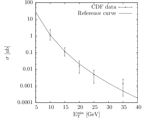
CDF has measured the dijet central exclusive cross section to be about 1 nb at GeV, which is three orders of magnitude below the above estimate. It indicates that the Sudakov suppression indeed plays a crucial role in this process.
The Sudakov form factor enters the loop integral, and it reshapes the regions that contribute most to the amplitude. Before the introduction of the Sudakov form factor, the loop was dominated by the soft momenta due to factor. Now, the weight of the soft momenta is suppressed in Eq. (46):
| (49) |
As a result, the dominant -region shifts towards harder scales. Using the saddle point approximation, it has been estimated [8] that the dominant region is at 1–2 GeV. It is often claimed that this makes the loop sufficiently hard to justify the applicability of pQCD and the usage of perturbative fits to the gluon density.
Here, we discuss this issue in some detail. With two simple estimates, we will show below that the overall suppression and the shift depend strongly on the details of the Sudakov form factor.
In the first approximation, the proton form factor plays the role of the infrared cut-off of the above integral: . Therefore, without the Sudakov form factor altogether, the integral in (50) is of order one.
Now, let us take the Sudakov form factor in the double-log approximation (22) with the fixed . Then,
| (51) |
and the position of the saddle point is at , i.e. the integral is still saturated in the soft region. The estimate of the suppression factor is then
which is about 0.2 for 10 GeV. If, instead, we take a running , then in the same double-log approximation
| (52) |
which gives now
| (53) |
which now makes typical 1 GeV. The integral then becomes
| (54) |
which is about for 10 GeV.
Such a severe qualitative change of the result clearly indicates its sensitivity to different prescriptions used in the Sudakov form factor. In the view of additional single-log corrections coming from unspecified scales in the logarithms as well as from the extra diagrams discussed in Section 2.3, which are not yet under control, one must conclude that the claims of perturbativity of the -loop are unjustified. Depending on the assumptions used, the Sudakov suppression can differ by one order of magnitude, and mean can vary from to GeV2. This uncertainty affects not only numerical results, but also some qualitative arguments.
Nevertheless, we see that it is possible to get a suppression factor of the order of 100 from the virtual corrections. This reduces our estimate to about 10 nb. An extra suppression of a factor 3 comes from the shift in when one goes from partons to jets. We shall discuss this in the next section. So we see that all the ingredients of this calculation can lead to a cross section in rough agreement with the data. In fact, we shall show that it is possible to get an exact agreement with the data, but that the number of adjustable theoretical corrections allows for many theoretical possibilities. Hence the CDF data turn out to be very important for tuning the theory.
6 Numerical results
6.1 Cuts
The two gluons produced through pomeron exchange hadronise into jets. As is unavoidable, this hadronisation can result in any number of jets, not just two. Theoretically, the difference between the two gluon cross section and the dijet cross section (i.e. the 3-jet veto) is a correction of the order of [46]. Given the large theoretical uncertainties in other parts of the calculation, we do not take this correction into account.
On the other hand, the transition from the partonic to the hadronic level involves corrections which are larger, and which are due to radiation outside the jet-finding cone — we shall generically refer to them as splash-out. The structure of these corrections is known [47, 48] and involves a constant shift in of the order of 1 GeV, due to hadronisation, as well as a correction proportional to due to radiation. The corresponding shift in has been estimated, for the cone algorithm used by CDF [49] to be
| (55) |
We shall also consider a previous parametrisation [50], where
| (56) |
One can then compare our results to the data, for which the cuts are summarised in Table 1.

(a) (b)
| [0.03, 0.08] | |
|---|---|
| , | [2.5,2.5] |
| , | |
| , |
We show in Fig. 9.b the effect of these corrections. We see that for the range of the CDF data, the effect of splash-out is non-negligible99 9 We thank V. Khoze for pointing this out to us. and amounts to a correction of the order of a factor of 3 for GeV, and the various possibilities for the splash-out bring in an uncertainty of the order of 1.7 at GeV to 4 at GeV. Note that the largest effect comes from the shift in . We have also considered a smearing in the rapidity of the jets, of the order of 1 unit, but this has an effect on the cross section of less than 0.1%. So it seems that in the longitudinal direction, the cuts of Table 1 can be directly applied at the parton level.
In the following, we shall fix the splash-out correction to . As a reference we shall also choose the parametrisation given in Table 2. This is not necessarily our best guess, but rather one of the choices which reproduces the CDF data. We shall include other possibilities when we extrapolate our results to the LHC.
| parameter | value | equation |
|---|---|---|
| 0.20 GeV | ||
| scale of in partonic cross section | ||
| scale of in Sudakov form factor | (19) | |
| angular ordering | yes | in (19) |
| terms in Sudakov exponentiation | constant+log+log2 | (19) |
| lower scale of Sudakov integral | (19) | |
| upper scale of Sudakov integral | (19) | |
| unintegrated structure function | ref. [36] | (30) |
| gap survival probability | (33) | |
| splash-out | (55) |
6.2 Properties of the amplitude
The accuracy of several properties and approximations presented in the literature can be directly tested from their effect on the cross section.


(a) (b)
The first property is the claim that the cross section is perturbative. We define as the value of the cross section in which all gluon momenta are larger than 1 GeV. Although this is not a physical observable, it is a useful quantity to test the assumptions used in theoretical calculations. We find that at CDF, the ratio is 0.35 for GeV, and falls to 0.25 for GeV. Clearly, as already mentioned, the effect of the Sudakov form factor is not sufficient to shift the dominant values of the momenta into the perturbative region, and we see that momenta below 1 GeV contribute significantly to the cross section. Note also that the larger , the softer the gluon loop. This is expected because at fixed proton energy, the production of higher- jets requires larger and , and it is a robust property of the unintegrated gluon distributions that they become softer at larger , see e.g.[34].
It might be, under those conditions, that modifications to the gluon propagator have to be taken into account [18]. It remains largely unclear however how to take these into account in a consistent and gauge-invariant way, as modifications to the propagator should also involve modifications to the vertices. Also, we have not taken into account the effect of the gap survival factor, which will reduce the dominant values of . Again, the formalism to follow seems unclear as the protons communicate with the jet via rather soft momenta.
The second point we can test is the neglect of the momenta in front of , which we used in our order-of-magnitude estimate (46). We show in Fig. 10.a that this approximation is very rough, and that it overestimates the cross section at high .
Finally, we confirm that the terms of the cross section (18) dominate the contributions, as noticed in [8]. The latter contribute 2% at GeV to 3% at GeV.
CDF also presented in [1] the dijet mass distribution of the jet system. Note that these are not true data but rather predictions of ExHuMe Monte Carlo simulations [51] normalised to the data: the ExHuMe cross section is normalised to the data in a given bin, and the distribution comes from summing over all these bins. The data is presented for GeV, i.e. where the lower cut has little influence. In Fig. 10.b, we show how our calculations compare with these distributions. We have produced two curves, both corresponding to minimum of 5 GeV, and assumed that the longitudinal splash-out is the same as the transverse one, i.e. we took . The first curve corresponds to our reference curve. It clearly overshoots the CDF points, and predicts a considerably harder spectrum than the ExHuMe Monte Carlo. The second curve goes perfectly though the points. The only difference is that in the latter case, the upper scale of the Sudakov form factor has been taken as , close to the choice of ExHuMe which takes , whereas in the former case that scale was . We see that the two choices of the scale lead to vastly different result, as they affect the dependence in of the cross section.
We argued in Section 2.2 that the upper scale in the Sudakov integral for the dijet production should be related with the relative transverse momentum rather than the invariant mass of the dijet. Thus, obtained from experimental data without the theoretical bias just described would help test this point.
6.3 Uncertainties
So far, we have shown that it is possible, with an appropriate choice of parameters, to reproduce the CDF dijet data via a calculation containing several perturbative ingredients, although the dominant momenta are largely in the non-perturbative region. We shall now see why this is the case: there is no firm reason to believe the parameters of Table 2, and different reasonable choices can easily lead to factors of a few up or down. Basically, all the lines of Table 2 can be changed to check on the resulting variation. We shall mention here only the most significant ones. We stress here that we are not trying to get the highest possible factor: our estimates are rather conservative, and based on changes that modest theoretical changes bring into the calculation.
The main correction comes from the inclusion of vertex corrections in the form of a Sudakov form factor. The upper and lower limits of the integral (19) can be modified while keeping single-log accuracy. We show in Fig. 11 the effect of such modifications.


(a) (b)
As we explained above, these plots clearly show that, in this region of , the vertex corrections lead to a rather uncertain situation. On the one hand, they are needed to reproduce the data, but on the other, their numerical impact depends on the details of their implementation. We estimate the uncertainty coming from variations of the limits of integration as about a factor 3 for the lower limit, and 6 for the upper one.
Furthermore, we show in Fig. 12.a the effect of changes in the choice of parametrisation. We first show the result of a resummation of log2 terms, including angular ordering, and choosing the scale of as . As we have seen before, the single-logs are opposite to the double logs, so that the cross section increases if one includes them. We also show in the same figure the change coming from choosing as the scale of in the Sudakov form factor. One sees that the choice of upper and lower limits in the Sudakov integral, and that of scale in can lead to much larger effects than the inclusion of subleading logs and constant terms.


(a) (b)
The second uncertainty comes from the impact factor, see Fig. 12.b. Several choices of unintegrated gluon densities, which differ only in the choice of parametrisation of soft colour-singlet exchange, lead to the shaded band, while the impact factor based on a simple 3-quark light-cone wave function leads to the curve. Although both lead to an acceptable fit to the CDF data, it seems that the curvature is better reproduced by the more sophisticated unintegrated gluon density. Uncertainties due to possible parametrisations of the soft region, and to the choice of form factor, amount to a factor of at least 3.
The parametrisations of the proton form factor used in this study contain a soft and a hard part. The hard part was obtained in [34, 35] within the -factorisation formalism, which is devised for processes with small- gluons and not too large transverse momenta. Although central exclusive production takes place precisely in this regime, one can, in principle, improve the treatment of the hard part in the spirit of the CCFM equation [27, 28], and one can imagine that this improvement will shift numerical results. However, we do not expect it to reduce the spread of different predictions because it comes mainly from our lack of knowledge of the proton form factor in the soft region.
To these uncertainties one must add that on the gap survival probability and that on the parametrisation of the splash-out, so that the overall theoretical uncertainty in the calculation is at least a factor 400 between the lowest and the highest estimates.
6.4 Predictions for the LHC
The formulae derived here can be equally used to estimate the central exclusive dijet production at the LHC. To do this, one needs to take into account the following corrections:
- •
Specific cuts that will be used at the LHC to search for such events. These are given in Table 3.
- •
Extrapolation of the proton form factor to the LHC energies. This can be done since the parametrisations of the unintegrated gluon distributions are available for very small .
- •
Extrapolation of the gap survival probability. For an estimate, we will use the prescription: .
The predictions for the LHC based solely on theoretical calculations will be unavoidably plagued by the same very large uncertainty as for the Tevatron. Restricting the models with the Tevatron data considerably reduces this uncertainty. In Fig. 13 we show our predictions for the dijet central exclusive production at the LHC. Shown are two bands indicating the range of uncertainties. The inner band represents how different sets of parameters, tuned at the Tevatron to describe the central value of the data, diverge as one extrapolates from the Tevatron to the LHC. The outer band includes all the parametrisations presented in the other figures of this paper which go through all the CDF points at the level.
We also checked that the ratio described in Section 6.2 is about 0.35 at the LHC, confirming that the gluon loop is still dominated by the soft region.
| cuts | A [52] | B [53] |
|---|---|---|
| [0.002,0.02] | [0.005,0.018] | |
| [0.002,0.02] | [0.004,0.014] | |
| GeV | GeV |


7 Conclusion
In this paper, we have seen that central exclusive production remains dominated by the non-perturbative region. This means that it is very important to use impact factors — such as the unintegrated gluon densities of [34, 35, 36] — which take the non-perturbative region into account. We have shown that this dominance of the soft region implies large uncertainties in all the ingredients of the calculation: vertex corrections, impact factors and screening corrections. We evaluate the uncertainty as being a factor 20 up or down, with no theoretically preferred curve.
At present, one can tune a perturbative calculation to the CDF run II data on dijet exclusive production, and try to use it to predict the cross sections for the production of other systems of particles.
There are several problems with this approach. The first one is that the huge Sudakov form factors of the dijet case suppress diagrams where the hard scale is concentrated in one propagator of the graph. Other graphs, such as those of Fig. 7, where the hard scale flows through the diagram, are suppressed by propagators, but one may expect the vertex corrections to be substantially smaller. So using dijet production as a handle on e.g. Higgs production may be misleading.
The second problem concerns the extrapolation to LHC energy. This is due to the fact that unitarisation effects will be important when going from 2 TeV to 14 TeV. The embedding of the process in a multi-pomeron environment can be achieved for short-distance hard partonic processes, leading to the usual gap survival probability. However in general, if the partons are not at very small distances, the gap survival probability will be more complicated, and larger. Also, it is usually assumed that Regge factorisation holds, i.e. that the process can be written as a product of factors depending on and , which is not the case here.
Clearly, all the above questions can only be settled by comparing to more data. Hence we believe that a measurement of quasielatic jet production at the LHC, including the rapidity distribution, the mass distribution, as well as the distribution, will be a very important task that will help to clarify many of the issues raised in this paper.
Acknowledgements
We thank M. Ryskin for communications and discussions about the lowest-order estimate and the Sudakov form factors, V. Khoze for pointing out the importance of the splash-out, and A. Papa for discussions about the general structure of jet production diagrams. We also acknowledge discussions with A. Martin, P.V. Landshoff, and K. Goulianos, and thank K. Terashi for private communications.
Appendices
Appendix A Lowest-order two-gluon production
in the quasi-multi-Regge kinematics
Consider the production of a colour-singlet two-gluon state in the collision. The two gluons are not required to have large transverse momenta or large invariant mass, but they are well separated in rapidity from the quarks. Besides, we require as usual that there is no overall colour flow in the -channel. Then, the kinematics and all the simplifications discussed in Sect. 1.1 and 1.2 still hold, and we are left with two generic diagrams shown in Fig. 4.
From the BFKL point of view, we deal with two-gluon production in the quasi-multi-Regge kinematics (qMRK). The imaginary part of the amplitude can be written as
| (57) | |||||
Here and are the usual Lipatov effective vertices (the tilde indicates that this vertex originates from the other -channel leg), e.g.
| (58) |
while is the effective RRGG vertex for two gluon production in qMRK [22]. In the multi-Regge kinematics (MRK) limit, , it factorizes into usual Lipatov vertices describing successive production of two MRK gluons:
| (59) |
On the other hand, when , one would recover from (57) the amplitude (8) described in the main text.
The two terms in (57) describe the respective contributions of the two generic diagrams of Fig. 4. Let us estimate how the contribution of the second diagram compares with the first one in the case of large and, for simplicity, at .
The square of the first diagram is
| (60) | |||||
For nearly forward scattering, , so that the estimate simplifies to
| (61) |
A similar estimate for the second diagram gives
| (62) | |||||
which for the forward case becomes
| (63) |
Thus, the second diagram is not only suppressed with respect to (61) by an extra power of , but also enhanced by an extra logarithm. If the loop corrections to this diagram can be resummed and presented in a form analogous to the Sudakov form factor, then the -integral will be shifted towards large values and no logarithmic enhancement in this new suppressing factor will occur. Hence the new Sudakov form factor may be much larger than the usual one.
Appendix B Intermediate production of gluons in multi-Regge
kinematics as
a source of corrections
to central exclusive production

If a colourless high-mass system can be “radiated” off the -channel gluons, then the same system can be produced via two intermediate gluons in multi-Regge kinematics (MRK) followed by their fusion into , see Fig. 8. We do not present here a detailed calculation of this process; however, it can be immediately seen from (4) and (57) that the resulting cross section is flat in rapidities of the intermediate gluons. Integrating over the corresponding lightcone variables but keeping fixed yields an extra longitudinal logarithm. The particular diagram shown in Fig. 14.a is in fact a double-log-enhanced correction to the direct production of system . In the standard calculation it is effectively included via the Sudakov form factor.
Even higher-order corrections to this diagram include diagrams with extra gluon rungs that join the two -channel gluons. If these extra gluons are above or below the central subprocess, as in Fig. 14.b, they can be absorbed into the definition of the unintegrated gluon density. However, if the gluon is attached inside the central subprocess, Fig. 14.c, it leads to a correction to the effective vertex and cannot be absorbed into the gluon density.
This correction is enhanced by a single logarithm. If the lightcone variables of the two intermediate gluons are , then the logarithm that appears is of type
where is the (moderate) transverse momentum of the intermediate gluons. Thus, this diagram represents a single-log enhanced correction to the central exclusive production of system , which involves the screening gluons and which is absent in the pure process. Since the single-log enhanced terms in the Sudakov integral are very important for the kinematic range considered, one must take seriously such corrections.
As the production of two gluons in MRK requires gluon emission from both -channel legs, one encounters additional single-log enhanced diagrams such as shown in Fig. 14.d.
We would like also to stress that, even without the above estimates, there is a need to evaluate such “non-conventional” diagrams, which stems directly from self-consistency of one’s approach. Indeed, if one believes the diagrams such as Fig. 14.d are not logarithmically enhanced, then the bare diagram Fig. 8.c does not get suppressed at all. It can then become comparable with the usual Sudakov-suppressed diagrams, as was explained in Section 2.3. If, on the other hand, Fig. 14.d and similar diagrams are logarithmically enhanced, one needs to resum them to estimate their effect.
References
- [1] T. Aaltonen et al. [CDF Run II Collaboration], Phys. Rev. D 77 (2008) 052004 [arXiv:0712.0604 [hep-ex]].
- [2] A. Schäfer, O. Nachtmann and R. Schöpf, Phys. Lett. B 249, 331 (1990).
- [3] J. D. Bjorken, Phys. Rev. D 47 (1993) 101.
- [4] A. Bialas and P. V. Landshoff, Phys. Lett. B 256 (1991) 540.
- [5] J. R. Cudell and O. F. Hernández, Nucl. Phys. B 471, 471 (1996) [arXiv:hep-ph/9511252].
- [6] A. Berera and J. C. Collins, Nucl. Phys. B 474, 183 (1996) [arXiv:hep-ph/9509258].
- [7] D. Kharzeev and E. Levin, Phys. Rev. D 63, 073004 (2001) [arXiv:hep-ph/0005311].
- [8] V. A. Khoze, A. D. Martin and M. G. Ryskin, Eur. Phys. J. C 14, 525 (2000) [arXiv:hep-ph/0002072]; Eur. Phys. J. C 19, 477 (2001) [Erratum-ibid. C 20, 599 (2001)] [arXiv:hep-ph/0011393].
- [9] B. Cox, J. R. Forshaw and B. Heinemann, “Double diffractive Higgs and di-photon production at the Tevatron and Phys. Lett. B 540, 263 (2002) [arXiv:hep-ph/0110173].
- [10] M. Boonekamp, R. Peschanski and C. Royon, Phys. Rev. Lett. 87, 251806 (2001) [arXiv:hep-ph/0107113].
- [11] M. Boonekamp, R. Peschanski and C. Royon, Nucl. Phys. B 669, 277 (2003) [Erratum-ibid. B 676, 493 (2004)] [arXiv:hep-ph/0301244].
- [12] M. Boonekamp, R. Peschanski and C. Royon, “Sensitivity to the standard model Higgs boson in exclusive double Phys. Lett. B 598, 243 (2004) [arXiv:hep-ph/0406061].
- [13] N. Timneanu, R. Enberg and G. Ingelman, Acta Phys. Polon. B 33, 3479 (2002) [arXiv:hep-ph/0206147].
- [14] R. Enberg, G. Ingelman, A. Kissavos and N. Timneanu, Phys. Rev. Lett. 89, 081801 (2002) [arXiv:hep-ph/0203267].
- [15] R. Enberg, G. Ingelman and N. Timneanu, Phys. Rev. D 67, 011301 (2003) [arXiv:hep-ph/0210408].
- [16] R. B. Appleby and J. R. Forshaw, Phys. Lett. B 541, 108 (2002) [arXiv:hep-ph/0111077].
- [17] R. J. M. Covolan and M. S. Soares, Phys. Rev. D 67, 077504 (2003) [arXiv:hep-ph/0305186].
- [18] A. Bzdak, Acta Phys. Polon. B 35, 1733 (2004) [arXiv:hep-ph/0404153]; Phys. Lett. B 608, 64 (2005) [arXiv:hep-ph/0407193]; Phys. Lett. B 615 (2005) 240 [arXiv:hep-ph/0504086].
- [19] S. M. Troshin and N. E. Tyurin, Eur. Phys. J. C 39 (2005) 435 [arXiv:hep-ph/0403021].
- [20] L. Frankfurt, C. E. Hyde-Wright, M. Strikman and C. Weiss, Phys. Rev. D 75 (2007) 054009 [arXiv:hep-ph/0608271].
- [21] V. S. Fadin, E. A. Kuraev and L. N. Lipatov, Phys. Lett. B 60 (1975) 50; I. I. Balitsky and L. N. Lipatov, Sov. J. Nucl. Phys. 28, 822 (1978) [Yad. Fiz. 28, 1597 (1978)].
- [22] V. S. Fadin and L. N. Lipatov, Sov. J. Nucl. Phys. 50, 712 (1989) [Yad. Fiz. 50, 1141 (1989)].
- [23] S. J. Parke and T. R. Taylor, Phys. Rev. Lett. 56 (1986) 2459.
- [24] V. V. Sudakov, Sov. Phys. JETP 3 (1956) 65 [Zh. Eksp. Teor. Fiz. 30 (1956) 87]; N. N. Bogoliubov, and D. V. Shirkov, Introduction to the theory of quantized fields (John Wiley, New York, 1980).
- [25] Y. L. Dokshitzer, D. Diakonov and S. I. Troian, Phys. Rept. 58 (1980) 269.
- [26] See for instance R.K. Ellis, W.J. Stirling and B. Webber, “QCD and Collider Physics”, Cambridge University Press, 1996, p. 165-185.
- [27] M. Ciafaloni, Nucl. Phys. B 296 (1988) 49; S. Catani, F. Fiorani and G. Marchesini, Phys. Lett. B 234 (1990) 339 and Nucl. Phys. B 336 (1990) 18.
- [28] M. A. Kimber, A. D. Martin and M. G. Ryskin, Phys. Rev. D 63 (2001) 114027 [arXiv:hep-ph/0101348]; M. A. Kimber, J. Kwiecinski, A. D. Martin and A. M. Stasto, Phys. Rev. D 62 (2000) 094006 [arXiv:hep-ph/0006184].
- [29] J. C. Collins, Adv. Ser. Direct. High Energy Phys. 5, 573 (1989) [arXiv:hep-ph/0312336]; A. Sen, Phys. Rev. D 24 (1981) 3281; G. P. Korchemsky, Phys. Lett. B 220 (1989) 629.
- [30] B. I. Ermolaev, M. Greco, F. Olness and S. I. Troyan, Phys. Rev. D 72 (2005) 054001.
- [31] H. Cheng and T. T. Wu, “Expanding protons: scattering at high energies”, Cambridge, USA: MIT Press (1987) 285p.
- [32] J. F. Gunion and D. E. Soper, Phys. Rev. D 15 (1977) 2617, E. M. Levin and M. G. Ryskin, Yad. Fiz. 34 (1981) 1114.
- [33] J. R. Cudell and B. U. Nguyen, Nucl. Phys. B 420 (1994) 669 [arXiv:hep-ph/9310298].
- [34] I. P. Ivanov and N. N. Nikolaev, Phys. Rev. D 65 (2002) 054004.
- [35] I. P. Ivanov, Ph. D. thesis, Bonn University, 2002, “Diffractive production of vector mesons in deep inelastic scattering within k(t)-factorization approach,” arXiv:hep-ph/0303053.
- [36] I. P. Ivanov, N. N. Nikolaev and A. A. Savin, Phys. Part. Nucl. 37 (2006) 1.
- [37] I. T. Drummond, P. V. Landshoff and W. J. Zakrzewski, Nucl. Phys. B 11 (1969) 383; Phys. Lett. B 28 (1969) 676.
- [38] M. Gluck, E. Reya and A. Vogt, Eur. Phys. J. C 5, 461 (1998).
- [39] A. D. Martin et al, Phys. Lett. B 443, 301 (1998).
- [40] H. L. Lai and W. K. Tung, Z. Phys. C 74, 463 (1997).
- [41] A. V. Radyushkin, Phys. Lett. B 449 (1999) 81 [arXiv:hep-ph/9810466]; A. G. Shuvaev, K. J. Golec-Biernat, A. D. Martin and M. G. Ryskin, Phys. Rev. D 60 (1999) 014015 [arXiv:hep-ph/9902410].
- [42] J. Kwiecinski and A. Szczurek, Nucl. Phys. B 680 (2004) 164 [arXiv:hep-ph/0311290].
- [43] F. Abe et al. [CDF Collaboration], Phys. Rev. D 50, 5518 (1994).
- [44] C. Avila et al. [E-811 Collaboration], Phys. Lett. B 537 (2002) 41.
- [45] For a recent review, see A. Achilli, R. Hegde, R. M. Godbole, A. Grau, G. Pancheri and Y. Srivastava, Phys. Lett. B 659 (2008) 137 [arXiv:0708.3626 [hep-ph]].
- [46] V. A. Khoze, A. D. Martin and M. G. Ryskin, JHEP 0605 (2006) 036 [arXiv:hep-ph/0602247].
- [47] J. M. Campbell, J. W. Huston and W. J. Stirling, Rept. Prog. Phys. 70 (2007) 89 [arXiv:hep-ph/0611148].
- [48] M. Dasgupta, L. Magnea and G. P. Salam, JHEP 0802 (2008) 055 [arXiv:0712.3014 [hep-ph]].
- [49] K. Terashi’s result, mentioned in V. A. Khoze, A. D. Martin and M. G. Ryskin, arXiv:0705.2314 [hep-ph].
- [50] V. A. Khoze, A. B. Kaidalov, A. D. Martin, M. G. Ryskin and W. J. Stirling, arXiv:hep-ph/0507040.
- [51] J. Monk and A. Pilkington, Comput. Phys. Commun. 175 (2006) 232 [arXiv:hep-ph/0502077].
- [52] M. G. Albrow et al., FP420 LOI, report CERN-LHCC-2005-025.
- [53] B. E. Cox, F. K. Loebinger and A. D. Pilkington, JHEP 0710 (2007) 090 [arXiv:0709.3035 [hep-ph]].