Iteratively Re-weighted Least Squares Minimization for Sparse Recovery
Abstract
Under certain conditions (known as the Restricted Isometry Property or RIP) on the -matrix (where ), vectors that are sparse (i.e. have most of their entries equal to zero) can be recovered exactly from even though is typically an -dimensional hyperplane; in addition is then
equal to the element in of minimal
-norm. This minimal element can be identified via linear programming algorithms.
We study an alternative method of determining , as the limit of an
Iteratively Re-weighted Least Squares (IRLS) algorithm.
The main step of this IRLS finds, for a given weight vector , the element
in with smallest -norm. If is the solution at iteration step , then the new weight is defined by
, , for a decreasing
sequence of adaptively defined ; this updated weight is then used to obtain and the process is repeated. We prove that when
satisfies the RIP conditions, the sequence converges for all
, regardless of
whether contains a sparse vector. If there is a sparse
vector in , then the limit is this sparse vector, and
when is sufficiently close to the limit, the remaining steps of the algorithm converge exponentially fast (linear convergence in the terminology of numerical optimization).
The same algorithm with the “heavier” weight
, , where , can recover sparse solutions as well;
more importantly, we show its local convergence is superlinear and approaches a
quadratic rate for approaching to zero.
1 Introduction
Let be an matrix with and let . (In the compressed sensing application that motivated this study, typically has full rank, i.e. . We shall implicitly assume, throughout the paper, that this is the case. Our results still hold for the case where , with the proviso that must then lie in .)
The linear system of equations
| (1.1) |
is underdetermined, and has infinitely many solutions. If is the null space of and is any solution to (1.1) then the set of all solutions to (1.1) is given by .
In the absence of any other information, no solution to (1.1) is to be preferred over any other. However, many scientific applications work under the assumption that the desired solution is either sparse or well approximated by (a) sparse vector(s). Here and later, we say a vector has sparsity (or is -sparse) if it has at most nonzero coordinates. Suppose then that we know that the desired solution of (1.1) is -sparse, where is known. How could we find such an ? One possibility is to consider any set of column indices and find the least squares solution , where is obtained from by setting to zero all entries that are not in columns from . Finding is numerically simple (see (1.9)). After finding each , we choose the particular set that minimizes the residual . This would find a -sparse solution (if it exists), . However, this naive method is numerically prohibitive when and are large, since it requires solving least squares problems.
An attractive alternative to the naive minimization is its convex relaxation that consists in selecting the element in which has minimal -norm:
| (1.2) |
Here and later we use the -norms
| (1.3) |
Under certain assumptions on and that we shall describe in §2, it is known that (1.2) has a unique solution (which we shall denote by ), and that, when there is a -sparse solution to (1.1), (1.2) will find this solution [3, 7, 20, 21]. Because the problem (1.2) can be formulated as a linear program, it is numerically tractable.
Solving underdetermined systems by -minimization has a long history. It is at the heart of many numerical algorithms for approximation, compression, and statistical estimation. The use of the -norm as a sparsity-promoting functional can be found first in reflection seismology and in deconvolution of seismic traces [16, 37, 38]. Rigorous results for -minimization began to appear in the late-1980’s, with Donoho and Stark [23] and Donoho and Logan [22]. Applications for -minimization in statistical estimation began in the mid-1990’s with the introduction of the LASSO and related formulations [39] (iterative soft-thresholding), also known as Basis Pursuit [15], proposed in compression applications for extracting the sparsest signal representation from highly overcomplete frames. Around the same time other signal processing groups started using -minimization for the analysis of sparse signals; see, e.g. [32]. The applications and understanding of -minimization saw a dramatic increase in the last 5 years [20, 24, 21, 25, 7, 4, 3, 6], with the development of fairly general mathematical frameworks in which -minimization, known heuristically to be sparsity-promoting, can be proved to recover sparse solutions exactly. We shall not trace all the relevant results and applications; a detailed history is beyond the scope of this introduction. We refer the reader to the survey papers [5, 1]. The reader can also find a comprehensive collection of the ongoing recent developments at the web-site http://www.dsp.ece.rice.edu/cs/. In fact, -minimization has been so surprisingly effective in several applications, that Candès, Wakin, and Boyd call it the “modern least squares” in [8]. We thus clearly need efficient algorithms for the minimization problem (1.2).
Several alternatives to (1.2), see, e.g., [26, 31], have been proposed as possibly more efficient numerically, or simpler to implement by non-experts, than standard algorithms for linear programming (such as interior point or barrier methods). In this paper we clarify fine convergence properties of one such alternative method, called Iteratively Re-weighted Least Squares minimization (IRLS). It begins with the following observation (see §2 for details). If (1.2) has a solution that has no vanishing coordinates, then the (unique!) solution of the weighted least squares problem
| (1.4) |
coincides with . (The following argument provides a short proof by contradiction of this statement. Assume that is not the -minimizer. Then there exists such that or equivalently . However, because is an -minimizer, we have for all ; taking sufficiently small, this implies , a contradiction.)
Since we do not know , this observation cannot be used directly. However, it leads to the following paradigm for finding . We choose a starting weight and solve (1.4) for this weight. We then use this solution to define a new weight and repeat this process. An IRLS algorithm of this type appears for the first time in the approximation practice in the Ph.D. thesis of Lawson in 1961 [30], in the form of an algorithm for solving uniform approximation problems, in particular by Chebyshev polynomials, by means of limits of weighted –norm solutions. This iterative algorithm is now well-known in classical approximation theory as Lawson’s algorithm. In [17] it is proved that this algorithm has in principle a linear convergence rate. In the 1970s extensions of Lawson’s algorithm for -minimization, and in particular -minimization, were proposed. In signal analysis, IRLS was proposed as a technique to build algorithms for sparse signal reconstruction in [28]. Perhaps the most comprehensive mathematical analysis of the performance of IRLS for -minimization was given in the work of Osborne [33].
Osborne proves that a suitable IRLS method is convergent for . For , if denotes the weight at the th iteration and the minimal weighted least squares solution for this weight, then the algorithm considered by Osborne defines the new weight coordinatewise as . His main conclusion in this case is that if the minimization problem (1.2) has a unique solution, then the algorithm converges to this solution, in principle with linear convergence rate, i.e. exponentially fast, with a constant “contraction factor”.
However, the analysis of Osborne does not take into consideration what happens if one of the coordinates vanishes at some iteration , i.e. . Taking this to impose that the corresponding weight component must “equal” leads to at the next iteration as well; this then persists in all later iterations. If , all is well, but if there is an index for which , yet at some iteration step , then this “infinite weight” prescription leads to problems. In practice, this is avoided by changing the definition of the weight at coordinates where (see [31] and [10, 27] where a variant for total variation minimization is studied); such modified algorithms need no longer converge to , however). Because Osborne’s convergence proof is local, it implies that if the iterations begin with a vector sufficiently close to the solution, and if the solution is unique and has only nonzero entries, then none of the vanish, and the weight-change is not required; Osborne’s analysis does indeed show the linear convergence rate of the algorithm under these assumptions. Unfortunately, as we will see in Remark 2.2, the uniqueness of the solution necessarily implies that it has vanishing components. In other words, the set of vectors to which Osborne’s analysis applies is vacuous.
The purpose of the present paper is to put forward an IRLS algorithm that gives a re-weighting without infinite components in the weight, and to provide an analysis of this algorithm, with various results about its convergence and rate of convergence. It turns out that care must be taken in just how the new weight is derived from the solution of the current weighted least squares problem. To manage this difficulty, we shall consider a very specific recipe for generating the weights. Other recipes are certainly possible.
Given a real number and a weight vector , with , , we define
| (1.5) |
Given and , the element that minimizes is unique because is strictly convex.
Our algorithm will use an alternating method for choosing minimizers and weights based on the functional . To describe this, we define for the non-increasing rearrangement of the absolute values of the entries of . Thus is the -th largest element of the set , and a vector is -sparse iff .
Algorithm 1
We initialize by taking . We also set . We then recursively define for
| (1.6) |
and
| (1.7) |
where is a fixed integer that will be described more fully later. We also define
| (1.8) |
We stop the algorithm if ; in this case we define for . However, in general, the algorithm will generate an infinite sequence of distinct vectors.
Each step of the algorithm requires the solution of a least squares problem. In matrix form
| (1.9) |
where is the diagonal matrix whose -th diagonal entry is and denotes the transpose of the matrix . Once is found, the weight is given by
| (1.10) |
We shall prove several results about the convergence and rate of convergence of this algorithm. This will be done under the following assumption on .
The Restricted Isometry Property (RIP): We say that the matrix satisfies the Restricted Isometry Property of order with constant if for each vector with sparsity we have
| (1.11) |
The RIP was introduced by Candès and Tao [7, 4] in their study of compressed sensing and -minimization. It has several analytical and geometrical interpretations that will be discussed in §3. To mention just one of these results (see [18]), it is known that if has the RIP of order , with (here ) and if (1.1) has a -sparse solution , then this solution is the unique minimizer in . (This can still be sharpened: in [9], Candès showed that if contains a -sparse vector, and if has RIP of order with , then that -sparse vector is unique and is the unique minimizer in .)
The main result of this paper (Theorem 5.3) is that whenever satisfies the RIP of order (for some ) and sufficiently close to zero, then Algorithm 1 converges to a solution of (1.1) for each . Moreover, if there is a solution to (1.1) that has sparsity , then . Here depends on the RIP constant and can be made arbitrarily close to when is made small. The result cited in our previous paragraph implies that in this case , where is the -minimal solution to (1.1).
A second part of our analysis concerns rates of convergence. We shall show that if (1.1) has a -sparse solution with, e.g., and if satisfies the RIP of order with sufficiently close to zero, then Algorithm 1 converges exponentially fast to . Namely, once is sufficiently close to its limit , we have
| (1.12) |
where is a fixed constant (depending on ). From this result it follows that we have exponential convergence to whenever is -sparse; however we have no real information on how long it will take before the iterates enter the region where we can control . (Note that this is similar to convergence results for the interior point algorithms that can be used for direct -minimization.)
The potential of IRLS algorithms, tailored to mimic -minimization and so recover sparse solutions, has recently been investigated numerically by Chartrand and several co-authors [11, 12, 14]. Our work provides proofs of several findings listed in these works.
One of the virtues of our approach is that, with minor technical modifications, it allows a similar detailed analysis of IRLS algorithms with weights that promote the non-convex optimization of -norms for . We can show not only that these algorithms can again recover sparse solutions, but also that their local rate of convergence is superlinear and tends to quadratic when tends to zero. Thus we also justify theoretically the recent numerical results by Chartrand et al. concerning such non-convex -norm optimization [11, 12, 13, 36].
An outline of our paper is the following. In the next section we make some remarks about - and weighted -minimization, upon which we shall call in our proof. In the following section, we recall the Restricted Isometry Property and the Null Space Property including some of its consequences that are important to our analysis. In section 4, we gather some preliminary results we shall need to prove our main convergence result, Theorem 5.3, which is formulated and proved in section 5. We then turn to the issue on rate of convergence in section 6. In section 7 we generalize the convergence results obtained for -minimization to the case of -spaces for ; in particular, we show, with Theorem 7.9, the local superlinear convergence of the IRLS algorithm in this setting. We conclude the paper with a short section dedicated to a few numerical examples that dovetail nicely with the theoretical results.
2 Characterization of - and weighted -minimizers
We fix and consider the underdetermined system . Given a norm , the problem of minimizing over can be viewed as a problem of approximation. Namely, for any , we can characterize the minimizers in as exactly those elements that can be written as , with a best approximation to from . In this way one can characterize minimizers from classical results on best approximation in normed spaces. We consider two examples of this in the present section, corresponding to the -norm and the weighted -norm.
Throughout this paper, we shall denote by any element from that has smallest -norm, as in (1.2). When is unique, we shall emphasize this by denoting it by . In general, and need not be sparse, although we will often consider cases where they are. We begin with the following well-known lemma (see for example Pinkus [34]) which characterizes the minimal -norm elements from .
Lemma 2.1
An element has minimal -norm among all elements if and only if
| (2.1) |
Moreover, is unique if and only if we have strict inequality in (2.1) for all which are not identically zero.
Proof: We give the simple proof for completeness of this paper. If has minimum -norm, then we have, for any and any ,
| (2.2) |
Fix . If is sufficiently small then and will have the same sign whenever . Hence, (2.2) can be written as
Choosing of an appropriate sign, we see that (2.1) is a necessary condition.
For the opposite direction, we note that if (2.1) holds then for each , we have
| (2.3) | |||||
| (2.4) |
where the first inequality uses (2.1).
If is unique then we have strict inequality in (2.2) and hence subsequently in (2.1). If we have strict inequality in
(2.1) then the subsequent strict inequality in (2.3)
implies uniqueness.
Remark 2.2
Applying Lemma 2.1 to the special case of -minimizers with no vanishing entries, we see that a vector , with for all , is a minimal -norm solution if and only if
| (2.5) |
This implies that a minimal -norm solution to for which all entries are non-vanishing is necessarily non-unique, by the following argument. Suppose that for all and that is a minimal -norm solution. Pick now any , , and pick so that ; it then follows that for all . But then we have by (2.5), so that is also a minimal solution, different from . Hence, unique -minimizers are necessarily -sparse for some .
We next consider minimization in a weighted -norm. We suppose that the weight is strictly positive which we define to mean that for all . In this case, is a Hilbert space with the inner product
| (2.6) |
We define
| (2.7) |
Because the -norm is strictly convex, the minimizer is necessarily unique; it is completely characterized by the orthogonality conditions
| (2.8) |
Namely, necessarily satisfies (2.8); on the other hand, any element that satisfies for all is automatically equal to .
At this point, we would like to tabulate some of the notation we have used in this paper to denote various kinds of minimizers and other solutions alike (such as limits of algorithms).
3 The Restricted Isometry and the Null Space Properties
To analyze the convergence of our algorithm, we shall impose the Restricted Isometry Property (RIP) already mentioned in the introduction, or a slightly weaker version, the Null Space Property, which will be defined below. Recall that satisfies RIP of order for (see (1.11)) iff
| (3.1) |
It is known that many families of matrices satisfy the RIP. While there are deterministic families that are known to satisfy RIP, the largest range of , (asymptotically, as , with e.g. kept constant) is obtained (to date) by using random families. For example, random families in which the entries of the matrix are independent realizations of a (fixed) Gaussian or Bernoulli random variable are known to have the RIP with high probability for each (see [7, 4, 2, 35] for a discussion of these results).
We shall say that has the Null Space Property (NSP) of order for if 11 1 This definition of the Null Space Property is a slight variant of that given in [18] but is more convenient for the results in the present paper.
| (3.2) |
for all sets of cardinality not exceeding and all . Here and later, we denote by the vector obtained from by setting to zero all coordinates for ; denotes the complement of the set . It is shown in Lemma 4.1 of [18] that if has the RIP of order for a given , where are integers, then has the NSP of order for . Note that if is sufficiently large then .
Another result in [18] (see also Lemma 4.3 below)
states
that in order to guarantee that a -sparse
vector is the unique -minimizer in , it is
sufficient that has the NSP of order and .
(In fact, the argument in [4], proving that for
with the RIP, -minimization
identifies sparse vectors in , can be split into two steps: one that
implicitly derives the NSP
from the RIP, and the remainder of the proof, which uses only the NSP.)
Note that if the NSP holds for some order and constant (not necessarily ),
then, by choosing
sufficiently small, one can ensure that has the NSP of order
with constant
(see [18] for details).
So the effect of requiring that is tantamount to reducing the range of
slightly.
When proving results on the convergence of our algorithm later in this paper, we shall state them under the assumptions that has the NSP for some and an appropriate value of . Using the observations above, they can easily be rephrased in terms of RIP bounds for .
4 Preliminary results
We first make some comments about the decreasing rearrangement and the -term approximation errors for vectors in . Let us denote by the set of all such that . For any and any , we denote by
| (4.1) |
the -error in approximating a general vector by a -sparse vector. Note that these approximation errors can be written as a sum of entries of : . We have the following lemma:
Lemma 4.1
The map is Lipschitz continuous on : for any , we have
| (4.2) |
Moreover, for any , we have
| (4.3) |
and for any , we have
| (4.4) |
Proof: For any pair of points and , and any , let be a set of indices corresponding to the largest entries in . Then
| (4.5) |
We can also reverse the roles of and . Therefore, we obtain (4.2). To prove (4.3), we approximate by a -term best approximation of in . Then
and the result follows from symmetry.
To prove (4.4), it suffices to note that
.
Our next result is an approximate reverse triangle inequality for points in . Its importance to us lies in its implication that whenever two points have close -norms and one of them is close to a -sparse vector, then they necessarily are close to each other. (Note that it also implies that the other vector must then also be close to that -sparse vector.) This is a geometric property of the null space.
Lemma 4.2
Assume that (3.2) holds for some and . Then, for any , we have
| (4.6) |
Proof: Let be a set of indices of the largest entries in . Then
| (4.7) | |||||
| (4.8) | |||||
| (4.9) | |||||
| (4.10) | |||||
| (4.11) |
Using (3.2), this gives
| (4.12) |
In other words,
| (4.13) |
Using this, together with (4.7), we obtain
| (4.14) |
as desired.
This result then allows the following simple proof of some of the results of [18]:
Lemma 4.3
Assume that (3.2) holds for some and . Suppose that contains an -sparse vector. Then this vector is the unique -minimizer in ; denoting it by , we have moreover, for all ,
| (4.15) |
Proof:
For the time being, we denote the -sparse vector in by .
Applying (4.6) with and , we find
since is arbitrary, this implies that for all , so that is an -norm minimizer in .
If were another -minimizer in , then it would follow that , and the inequality we just derived would imply , or . It follows that is the unique -minimizer in , which we denote by , as proposed earlier.
Our next set of remarks centers around the functional defined by (1.5). Note that for each , we have
| (4.16) |
We also have the following monotonicity property which holds for all :
| (4.17) |
Here the first inequality follows from the minimization property that defines , the second inequality from , and the last inequality from the minimization property that defines . For each , is completely determined by ; for , in particular, is determined solely by , and independent of the choice of . (With the initial weight vector defined by , is the classical minimum -norm element of .) The inequality (4.17) for thus holds for arbitrary .
Lemma 4.4
For each we have
| (4.18) |
and
| (4.19) |
5 Convergence of the algorithm
In this section, we prove that the algorithm converges. Our starting point is the following lemma that establishes for .
Lemma 5.1
Proof: For each , we have
| (5.3) | |||||
| (5.4) | |||||
| (5.5) | |||||
| (5.6) | |||||
| (5.7) | |||||
| (5.8) |
where the third equality uses the fact that
(observe that
and invoke (2.8)),
and the inequality uses the bound (4.19) on the weights. If we
now sum these inequalities over , we arrive
at (5.1).
From the monotonicity of , we know that exists and is non-negative. The following functional will play an important role in our proof of convergence:
| (5.9) |
Notice that if we knew that converged to then, in view of (4.16), would be the limit of . When the functional is strictly convex and therefore has a unique minimizer
| (5.10) |
This minimizer is characterized by the following lemma:
Lemma 5.2
Let and . Then if and only if for all , where .
Proof: For the “only if” part, let and be arbitrary. Consider the analytic function
We have , and by the minimization property for all . Hence, . A simple calculation reveals that
which gives the desired result.
For the “if” part, assume that and for all , where is defined as above. We shall show that is a minimizer of on . Indeed, consider the convex univariate function . For any point we have from convexity that
| (5.11) |
because the right side is the linear function which is tangent to this function at . It follows that for any point we have
| (5.12) |
where we have used the orthogonality condition (5.18) and the fact
that is in .
Since is arbitrary, it follows that , as claimed.
We now give the convergence of the algorithm.
Theorem 5.3
Let (the same index as used in the update rule (1.7)) be chosen so that satisfies the Null
Space Property (3.2) of order , with .
Then, for each , the output of Algorithm 1 converges
to a vector , with
and the following hold:
(i) If , then is -sparse; in this
case there is therefore a unique -minimizer , and ;
moreover, we have, for , and any ,
| (5.13) |
(ii) If , then ;
(iii) In this last case, if satisfies the stricter bound
(or,
equivalently, if ), then we have, for all
and any , that
| (5.14) |
As a consequence, this case is excluded if contains a vector of sparsity .
The constant can be quite reasonable;
for instance, if and , then
we have .
Proof: Note that since , the always converge. We start by considering the case .
Case : In this case, we want to prove that converges , and that its limit is an -minimizer. Suppose that for some . Then by the definition of the algorithm, we know that the iteration is stopped at , and , . Therefore . From the definition of , it then also follows that and so is -sparse. As noted in §3 and Lemma 4.3, if a -sparse solution exists when satisfies the NSP of order with , then it is the unique -minimizer. Therefore, equals , this unique minimizer.
Suppose now that for all . Since , there is an increasing sequence of indices such that for all . By the definition (1.7) of , we must have for all . Noting that is a bounded sequence, there exists a subsequence of such that converges to a point . By Lemma 4.1, we know that converges to . Hence we get
| (5.15) |
which means that the support-width of is at most , i.e. is -sparse. By the same token used above, we again have that , the unique -minimizer. We must still show that . Since and , (4.16) implies . By the monotonicity property stated in (4.17), we get . Since (4.16) implies
| (5.16) |
we obtain . Finally, we invoke Lemma 4.2 with , , and to get
| (5.17) |
which completes the proof that in this case.
Case : We shall first show that , , with as defined by (5.10). By Lemma 4.4, we know that is a bounded sequence in and hence this sequence has accumulation points. Let be any convergent subsequence of and let be its limit. We want to show that .
Since , it follows that , . On the other hand, by invoking Lemma 5.1, we now find that , . It then follows from the orthogonality relations (2.8) that for every , we have
| (5.18) |
Now the “if” part of Lemma 5.2 implies that . Hence is the unique accumulation point of and therefore its limit. This establishes (ii).
To prove the error estimate (5.14) stated in (iii), we first note that for any , we have
| (5.19) |
where the second inequality uses the minimizing property of . Hence it follows that . We now invoke Lemma 4.2 to obtain
| (5.20) |
From Lemma 4.1 and (1.7), we obtain
| (5.21) |
It follows from (4.4) that
| (5.22) | |||||
| (5.23) | |||||
| (5.24) |
where the last inequality uses (5.20). Since by assumption on , we have , i.e. , we obtain
Finally, notice that if contains a -sparse vector (with ), then we know already (see §3) that this must be the unique -minimizer ; it then follows from our arguments above that we must have . Indeed, if we had , then (5.22) would hold for ; since is -sparse, , implying , a contradiction with the assumption . This finishes the proof.
Remark 5.4
Let us briefly compare our analysis of the IRLS algorithm with minimization. The latter recovers a -sparse solution (when one exists) if has the NSP of order and . The analysis given in our proof of Theorem 5.3 guarantees that our IRLS algorithm recovers -sparse for a slightly smaller range of values than -minimization, namely for . Notice that this “gap” vanishes for vanishingly small . Although we have no examples to demonstrate, our arguments cannot exclude the case where contains a -sparse vector with (e.g., if and ), and our IRLS algorithm converges to , yet . However, note that unless is close to 1, the range of -values in this “gap” is fairly small; for instance, for , this non-recovery of a -sparse can happen only if .
6 Rate of Convergence
Under the conditions of Theorem 5.3 the algorithm converges to a limit ; if there is a -sparse vector in with , then this limit coincides with that -sparse vector, which is then also automatically the unique -minimizer . In this section our goal is to establish a bound for the rate of convergence in both the sparse and non-sparse cases. In the latter case, the goal is to establish the rate at which approaches to a ball of radius centered at . We shall work under the same assumptions as in Theorem 5.3.
6.1 Case of -sparse vectors
Let us begin by assuming that contains the -sparse vector . The algorithm produces the sequence , which converges to , as established above. Let us denote the (unknown) support of the -sparse vector by .
We introduce an auxiliary sequence of error vectors via and
We know that . The following theorem gives a bound on the rate of convergence of to zero.
Theorem 6.1
Assume satisfies NSP of order with constant such that . Suppose that , , and are such that
Assume that contains a -sparse vector and let . Let be such that
| (6.1) |
Then for all , we have
Consequently converges to exponentially.
Remark 6.2
Notice that if is sufficiently small, e.g. , then for any , there is a for which , so we have exponential convergence to whenever is -sparse.
Proof: We start with the relation (2.8) with , , and , which gives
Rearranging the terms and using the fact that is supported on , we get
| (6.2) |
We will prove the theorem by induction. Let us assume that we have shown already. We then have, for all ,
so that
| (6.3) |
and hence (6.2) combined with (6.3) and NSP gives
At the same time, the Cauchy-Schwarz inequality combined with the above estimate yields
| (6.4) | |||||
If , then . In this case is -sparse and the algorithm has stopped by definition; since is in the null space , which contains no -sparse elements other than , we have already obtained the solution . If , then after canceling the factor in (6.4), we get
and thus
| (6.5) |
Now, we also have by (1.7) and (4.4)
| (6.6) |
since by assumption . This, together with (6.5), yields the desired bound,
In particular, since
, we have , which completes the induction step.
It follows that for all .
Remark 6.3
Note that the precise update rule (1.7) for does not really intervene in this analysis. If , then the estimate
| (6.7) |
guarantees that all further will be bounded by as well,
provided . It is only
in guaranteeing that (6.1) must be satisfied for some
that the update rule plays a role: indeed,
by Theorem 5.3, for
if is updated following (1.7), so that (6.1) has
to be satisfied eventually.
Other update rules may work as well. If is defined so
that it is a monotonically decreasing sequence with
limit , then the relation (6.7) immediately implies that
In particular, if , then . The rate at which in this case will depend on as well as on the rate with which . We shall not quantify this relation, except to note that if for some , then where .
6.2 Case of noisy -sparse vectors
We show here that the exponential rate of convergence to a -sparse limit vector can be extended to the case where the “ideal” (i.e. -sparse) target vector has been corrupted by noise and is therefore only “approximately -sparse”. More precisely, we no longer assume that contains a -sparse vector; consequently the limit of the need not be an -minimizer (see Theorem 5.3). If is any -minimizer in , Theorem 5.3 guarantees ; since this is the best level of accuracy guaranteed in the limit, we are in this case interested only in how fast will converge to a ball centered at with radius given by some (prearranged) multiple of . (Note that if contains several -minimizers, they all lie within a distance of each other, so that it does not matter which we pick.) We shall express the notion that is “approximately -sparse with gap ratio ”, or a “noisy version of a -sparse vector, with gap ratio ” by the condition
where is such that has the NSP for some pair such that (e.g. we could have if ). If the gap ratio is much greater than the constant in (5.14), then exponential convergence can be exhibited for a meaningful number of iterations. Note that this class includes perturbations of any -sparse vector for which the perturbation is sufficiently small in -norm (when compared to the unperturbed -sparse vector).
Our argument for the noisy case will closely resemble the case for the exact -sparse vectors. However there are some crucial differences that justify our decision to separate these two cases.
We will be interested in only the case where we recall that is the limit of the occurring in the algorithm, This assumption implies , and can only happen if is not -sparse. (As noted earlier, the exact -sparse case always corresponds to if . For in the region , both and are theoretical possibilities.)
First, we redefine , where is the minimizer of on and . We know from Theorem 5.3 that . We again set .
Theorem 6.4
Given , and integers with , assume that satisfies the NSP of order with constant such that all the conditions of Theorem 5.3 are satisfied and, in addition,
Suppose is “approximately -sparse with gap ratio ”, i.e.
| (6.8) |
with , where is as in Theorem 5.3. Let stand for the set of indices of the largest entries of , and be such that
| (6.9) |
Then for all , we have
| (6.10) |
where is a constant. Similarly, if we define , then
| (6.11) |
for , where is a constant. This implies that converges at an exponential (linear) rate to the ball of radius centered at .
Remark 6.5
Note that Theorem 5.3 trivially implies the inequalities (6.10) and (6.11) in the limit since , , and . However, Theorem 6.4 quantifies the event when it is guaranteed that the two measures of error, and , must shrink (at least) by a factor at each iteration. As noted above, this corresponds to the range , and would be realized if, say, is the sum of a -sparse vector and a fully supported “noise” vector which is sufficiently small in norm. In this sense, the theorem shows that the rate estimate of Theorem 5.3 extends to a neighborhood of -sparse vectors.
Proof: First, note that the existence of is guaranteed by the fact that and . For the latter, note that Lemma 4.1 and Theorem 5.3 imply
so that .
We follow the proof of Theorem 6.1 and consider the orthogonality relation (6.2). Since is not sparse in general, we rewrite (6.2) as
| (6.12) |
We deal with the contribution on in the same way as before:
For the contribution on , note that
Since we have . It follows that
| (6.13) |
where the second inequality is due to Lemma 4.1, the last one to Theorem 5.3, and . Combining these two bounds, we get
We combine this again with a Cauchy-Schwarz estimate, to obtain
| (6.14) | |||||
It is easy to check that if , where and are positive, then . Applying this to in the above estimate, we get
| (6.15) |
where . Similar to (6.6), we also have, by combining (4.4) with (part of) the chain of inequalities (6.13),
| (6.16) |
and consequently (6.15) becomes
| (6.17) | |||||
where . Since the are bounded, this gives
It then follows that if we pick so that , and consider the range of such that , then
Hence we are guaranteed exponential decay of as long as is sufficiently far from its limit. The smallest possible value of corresponds to the case .
To establish a rate of convergence to a comparably-sized ball centered at , we consider . It then follows that
| (6.18) | |||||
| (6.19) | |||||
| (6.20) | |||||
| (6.21) |
which shows the claimed exponential decay and also that
7 Beyond the convex case: -minimization for
If has the NSP of order with , then (see §3) -minimization recovers -sparse solutions to for any that admits such a -sparse solution, i.e., -minimization gives also -minimizers, provided their support has size at most . In [29], Gribonval and Nielsen showed that in this case, -minimization also gives the -minimizers, i.e., -minimization also solves non-convex optimization problems of the type
| (7.1) |
Let us first recall the results of [29] that are of most interest to us here, reformulated for our setting and notations.
Lemma 7.1
Lemma 7.2
([29, Theorem 5]). Let , , and . Then
Combining these two lemmas with the observations in §3 leads immediately to the following result.
Theorem 7.3
Fix any . If satisfies the NSP of order with constant then
| (7.2) |
for all and for all such that .
In addition, if , and if there exists a -sparse vector in , then this -sparse vector is the unique minimizer in of .
At first sight, these results suggest there is nothing to be gained by carrying out - rather than -minimization; in addition sparse recovery via the non-convex problems (7.1) is much harder than the more easily solvable convex relaxation problem of -minimization.
Yet, we shall show in this section that -minimization has unexpected benefits, and that it may be both useful and practically feasible via an IRLS approach. Before we start, it is expedient to introduce the following definition: we shall say that has the -Null Space Property (-NSP) of order with constant if, for all sets of cardinality at most and all ,
| (7.3) |
In what follows we shall construct an IRLS algorithm for - minimization. We shall see that
- (a)
In practice, -minimization can be carried out by an IRLS algorithm. Hence, the non-convexity does not necessarily make the problem intractable;
- (b)
In particular, if satisfies the -NSP of order , and if there exists a -sparse vector in , with for suitable given below, then the IRLS algorithm converges to the -minimizer , which, therefore, will coincide with ;
- (c)
Surprisingly the rate of local convergence of the algorithm is superlinear; the rate is larger for smaller , increasing to approach a quadratic regime as . More precisely, we will show that the local error satisfies
(7.4) where for sufficiently small. The validity of (7.4) is restricted to in a (small) ball centered at . In particular, if is close enough to then (7.4) ensures the convergence of the algorithm to the -sparse solution .
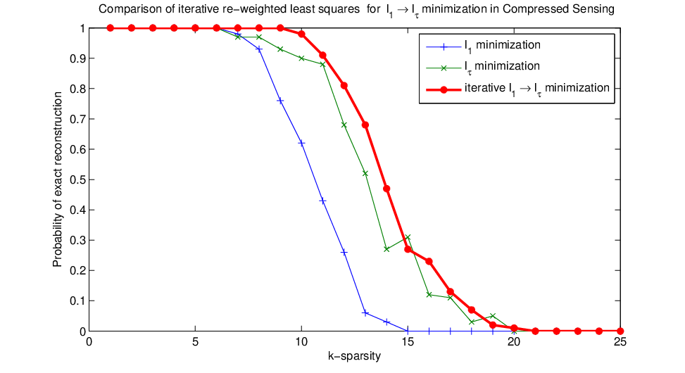
Some of these virtues of -minimization were recently highlighted by Chartrand and his collaborators [11, 12, 13]. Chartrand and Staneva [13] give a fine analysis of the RIP from which they can conclude that -minimization not only recovers -sparse vectors, but that the range of for which this recovery works is larger for smaller . Namely, for random Gaussian matrices, they prove that with high probability on the draw of the matrix sparse recovery by -minimization works for , where is bounded and decreases to zero as . In particular, the dependence of the sparsity on the number of columns vanishes for . These bounds give a quantitative estimate of the improvement provided by -minimization vis a vis -minimization for which the range of -sparsity for having exact recovery is clearly smaller (see Figure 8.4 for a numerical illustration).
7.1 Some useful properties of spaces
We start by listing in one proposition some fundamental and well-known properties of spaces for . For further details we refer the reader to, e.g., [19].
Proposition 7.4
(i) Assume . Then the map defines a quasi-norm for , in particular the triangle inequality holds up to a constant, i.e.,
| (7.5) |
If one considers the -th powers of the “-norm”, then one has the so-called “-triangle inequality”:
| (7.6) |
(ii) We have, for any
| (7.7) |
We will refer to this norm estimate by writing the embedding relation
.
(iii) (Generalized Hölder inequality) For and such that , and for a positive weight vector we have
| (7.8) |
where , as usual , for .
For technical reasons, it is often more convenient to employ the -triangle inequality (7.6) than (7.5); in this sense, for -minimization turns out to be more natural as a measure of error than the quasi-norm .
In order to prove the three claims (a)-(c) listed before the start of this subsection, we also need to generalize to certain results previously shown only for . In the following we assume . We denote by
the error of the best -term approximation to with respect to . As a straightforward generalization of analogous results valid for the -norm, we have the following two technical lemmas.
Lemma 7.5
For any , we have
for all . Moreover, for any , we have
Lemma 7.6
Assume that has the -NSP of order with constant . Then, for any , we have
7.2 An IRLS algorithm for -minimization
To define an IRLS algorithm promoting -minimization for a generic , we first define a -dependent functional , generalizing :
| (7.9) |
The desired algorithm is then defined simply by substituting for in Algorithm 1, keeping the same update rule (1.7) for . In particular we have
and
Fundamental properties of the algorithm are derived in the same way as before. In particular, the values decrease monotonically,
and the iterates are bounded,
As in Lemma 4.4, the weights are uniformly bounded from below, i.e.,
Moreover, using for in Lemma 5.1, we can again prove the asymptotic regularity of the iterations, i.e.,
The first significant difference with the -case arises when . In this latter situation, we need to consider the function
| (7.10) |
We denote by its set of minimizers on (since is no longer convex it may have more than one minimizer). Even though every minimizer still satisfies
where is defined by , , the converse need no longer be true.
The following theorem summarizes the convergence properties on the algorithm in the case .
Theorem 7.7
Fix . Let (the same index as in the update rule
(1.7) ) be chosen so that satisfies the -NSP of order with a constant such that . Let be the set of accumulation points of , and define . Then, the algorithm has the following properties:
(i) If , then consists of a single point , the converge to , and is an -minimizer in which is also -sparse.
(ii)
If , then for each we have
,
for all .
(iii) If and , we have
for all
.
Remark 7.8
Unlike Theorem 5.3, Theorem 7.7 does not ensure that the IRLS algorithm converges to the sparsest or to the minimal -solution. It does provide conditions that are verifiable a posteriori (e.g., ) for such convergence. The reason for this weaker result is the non-convexity of . (In particular, it might happen that is a local minimizer of , but not a global one, and the estimate in (iii) does not necessarily hold.) Nevertheless, as is often the case for non-convex problems, we can establish a local convergence result that also highlights the rate we can expect for such convergence. This is the content of the following section; it will be followed by numerical results that dovetail nicely with the theoretical results.
7.3 Local superlinear convergence
Throughout this section, we assume that there exists a -sparse vector in . We define the error vectors ; we now measure the error by :
Theorem 7.9
Proof: The proof is by induction on . We assume that and derive (7.13). As in the proof of Theorem 6.1, we let denote the support of and so and is the smallest entry in . Following the proof of Theorem 6.1, the first few lines are the same. The first difference is in the following estimate, which holds for and replaces (6.3),
Starting with the orthogonality relation (6.2) and using the above inequality and the embedding , we obtain
We now apply the -NSP to find
| (7.14) |
At the same time, the generalized Hölder inequality (see Proposition 7.4 (iii)) for and , together with the above estimates, yields
In other words,
| (7.15) |
Let us now estimate the weight term. By the -triangle inequality (7.6) we have
Now, an application of Lemma 7.5 gives the following estimates
Using these estimates in (7.15) gives
and (7.13) follows by a further application of the -NSP (see (6.5)).
Because of the assumption (7.12), we also have and so the induction can continue.
Remark 7.10
In contrast to the case, we do not need to ensure that decreases. In fact, all that is needed for the error reduction is for some sufficiently large . In fact, could be quite large in cases where the smallest non-zero component of the sparse vector is very small. We have not observed this effect in our examples; we expect that our analysis, although apparently accurate in describing the rate of convergence (see section 8), is too pessimistic in estimating the coefficient .
8 Numerical results
In this section we present numerical experiments that illustrate that the bounds derived in the theoretical analysis do manifest themselves in practice.
8.1 Convergence rates
We start with numerical results that confirm the linear rate of convergence of our iteratively re-weighted least square algorithm for -minimization, and its robust recovery of sparse vectors. In the experiments we used a matrix of dimensions and Gaussian i.i.d. entries. Such matrices are known to possess (with high probability) the RIP property with optimal bounds [2, 4, 35]. In Figure 8.1 we depict the approximation error to the unique sparsest solution shown in Figure 8.2, and the instantaneous rate of convergence. The numerical results both confirm the expected linear rate of convergence and the robust reconstruction of the sparse vector.
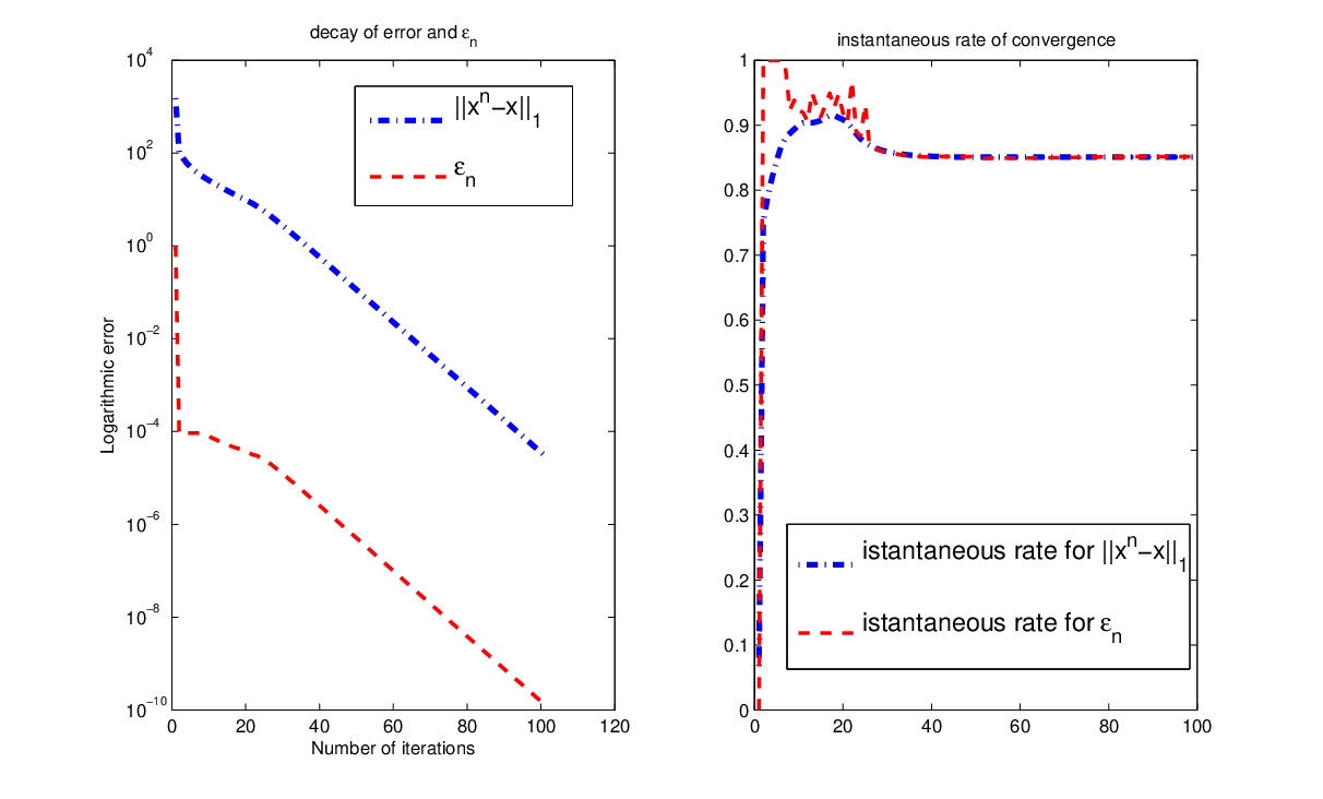

Next, we compare the linear convergence achieved with -minimization with the superlinear convergence obtained by the iteratively re-weighted least square algorithm promoting -minimization.
In Figure 8.3 we are interested in the comparison of the rate of convergence when our algorithm is used for different choices of . For and , the figure shows the error, as a function of the iteration step , for the iterative algorithm, with different fixed values of . For , the rate is linear, as in Figure 8.1. For the smaller values and the iterations initially follow the same linear rate; once they are sufficiently close to the sparse solution, the convergence rate speeds up dramatically, suggesting we have entered the region of validity of (7.13). For smaller values of numerical experiments do not always lead to convergence: in some cases the algorithm never got to the neighborhood of the solution where convergence is ensured. However, in this case a combination of initial iterations with the -inspired IRLS (for which we always have convergence) and later iterations with -inspired IRLS for smaller allow again for a very fast convergence to the sparsest solution; this is illustrated in Figure 8.3 for the case .

8.2 Enhanced recovery in compressed sensing and relationship with other work
Candès, Wakin, and Boyd [8] showed, by numerical experimentation, that iteratively re-weighted -minimization, with weights suggested by an -minimization goal, can enhance the range of sparsity for which perfect reconstruction of a sparse vector “works” in compressed sensing. In experiments with iteratively re-weighted -minimization algorithms, Chartrand and several collaborators observed a similar significant improvement [11, 12, 13, 14, 36]; see in particular [13, Section 4]; we also illustrate this in Figure 8.4.
It is to be noted that IRLS algorithms are computationally much less demanding than weighted -minimization. In addition, there is, as far as we know, no analysis (as yet) for re-weighted -minimization that is comparable to the detailed theoretical analysis of convergence presented here of our IRLS algorithm, which seems to give a realistic picture of the numerical computations.
9 Acknowledgments
We would like to thank Yu Chen, Michael Overton for various conversations on the topic of this paper, and Rachel Ward for pointing out an improvement of Theorem 5.3.
Ingrid Daubechies gratefully acknowledges partial support by NSF grants DMS-0504924 and DMS-0530865. Ronald DeVore thanks the Courant Institute for supporting an academic year visit when part of this work was done. He also gratefully acknowledges partial support by Office of Naval Research Contracts ONR-N00014-03-1-0051, ONR/DEPSCoR N00014-03-1-0675 and ONR/DEPSCoR N00014-00-1-0470; the Army Research Office Contract DAAD 19-02-1-0028; and the NSF contracts DMS-0221642 and DMS-0200187. Massimo Fornasier acknowledges the financial support provided by the European Union via the Individual Marie Curie fellowship MOIF-CT-2006-039438, and he thanks the Program in Applied and Computational Mathematics at Princeton University for its hospitality during the preparation of this work. Sinan Güntürk has been supported in part by the National Science Foundation Grant CCF-0515187, an Alfred P. Sloan Research Fellowship, and an NYU Goddard Fellowship.
References
- [1] R. Baraniuk, Compressive sensing, IEEE Signal Processing Magazine, (2007), vol. 24 no. 4, 118–121.
- [2] R. Baraniuk, M. Davenport, R. DeVore, and M. Waken, A simple proof of the restricted isometry property for random matrices, Constr. Approx., to appear
- [3] E. Candès, J. Romberg, and T. Tao, Stable signal recovery from incomplete and inaccurate measurements, Comm. Pure Appl. Math. 59 (2006), no. 8, 1207–1223.
- [4] E. Candès and T. Tao, Near optimal signal recovery from random projections: universal encoding strategies?, IEEE Trans. Inform. Theory 52 (2006), no. 12, 5406–5425.
- [5] E. J. Candès, Compressive sampling, International Congress of Mathematicians. Vol. III, Eur. Math. Soc., Zürich, 2006, pp. 1433–1452.
- [6] E. J. Candès, J. Romberg, and T. Tao, Exact signal reconstruction from highly incomplete frequency information, IEEE Trans. Inf. Theory 52 (2006), no. 2, 489–509.
- [7] E. J. Candès and T. Tao, Decoding by linear programming, IEEE Trans. Inform. Theory 51 (2005), no. 12, 4203–4215.
- [8] E. J. Candès, M. Wakin, and S. Boyd, Enhancing sparsity by reweighted minimization, (Technical Report, California Institute of Technology).
- [9] E.J. Candès, Lecture notes of the IMA course on Compressed Sensing, (2007), see http://www.ima.umn.edu/2006-2007/ND6.4-15.07/abstracts.html.
- [10] A. Chambolle and P.-L. Lions, Image recovery via total variation minimization and related problems., Numer. Math. 76 (1997), no. 2, 167–188.
- [11] R. Chartrand, Exact reconstructions of sparse signals via nonconvex minimization, IEEE Signal Process. Lett. 14 (2007), 707–710.
- [12] , Nonconvex compressive sensing and reconstruction of gradient-sparse images: random vs. tomographic Fourier sampling, preprint (2008).
- [13] R. Chartrand and V. Staneva, Restricted isometry properties and nonconvex compressive sensing, preprint (2008).
- [14] R. Chartrand and W. Yin, Iteratively reweighted algorithms for compressive sensing, Proceedings of the 33rd International Conference on Acoustics, Speech, and Signal Processing (ICASSP).
- [15] S. S. Chen, D. L. Donoho, and M. A. Saunders, Atomic decomposition by basis pursuit, SIAM J. Sci. Comput. 1 (1998), 33–61.
- [16] J. F. Claerbout and F. Muir, Robust modeling with erratic data, Geophysics 38 (1973), no. 5, 826–844.
- [17] A. K. Cline, Rate of convergence of Lawson’s algorithm, Math. Comp. 26 (1972), 167–176.
- [18] A. Cohen, W. Dahmen, and R. DeVore, Compressed sensing and best k-term approximation, J. Amer. Math. Soc., to appear.
- [19] R. DeVore, Nonlinear approximation, Acta Numerica 7 (1998), 51–150.
- [20] D. L. Donoho, Compressed sensing, IEEE Trans. Inf. Theory 52 (2006), no. 4, 1289–1306.
- [21] D. L. Donoho, High-dimensional centrally symmetric polytopes with neighborliness proportional to dimension, Discrete Comput. Geom. 35 (2006), no. 4, 617–652.
- [22] D. L. Donoho and B. F. Logan, Signal recovery and the large sieve, SIAM J. Appl. Math. 52 (1992), no. 2, 557–591.
- [23] D. L. Donoho and P. B. Stark, Uncertainty principles and signal recovery, SIAM J. Appl. Math. 49 (1989), no. 3, 906–931.
- [24] D. L. Donoho and J. Tanner, Sparse nonnegative solutions of underdetermined linear equations by linear programming, Proc. Nat. Acad. Sci. 102 (2005), no. 27, 9446–9451
- [25] , Counting faces of randomly-projected polytopes when the projection radically lowers dimension, preprint (2006).
- [26] D. L. Donoho and Y. Tsaig, Fast solution of -norm minimization problems when the solution may be sparse, preprint (2006).
- [27] M. Fornasier and R. March, Restoration of color images by vector valued BV functions and variational calculus, SIAM J. Appl. Math. 68 (2007), no. 2, 437–460.
- [28] I.F. Gorodnitsky and B.D. Rao. Sparse signal reconstruction from limited data using FOCUSS: a recursive weighted norm minimization algorithm, IEEE Transactions on Signal Processing, 45 (1997), no. 3, 600–616.
- [29] R. Gribonval and M. Nielsen, Highly sparse representations from dictionaries are unique and independent of the sparseness measure, Appl. Comput. Harmon. Anal. 22 (2007), no. 3, 335–355.
- [30] C. L. Lawson, Contributions to the Theory of Linear Least Maximum Approximation, Ph.D. thesis, University of California, Los Angeles, 1961.
- [31] Y. Li, A globally convergent method for problems, SIAM J. Optim. 3 (1993), no. 3, 609–629.
- [32] M.S. O’Brien, A.N. Sinclair and S.M. Kramer, Recovery of asparse spike time series by norm deconvolution, IEEE Trans. Signal Processing, 42 (1994), 3353–3365.
- [33] M. R. Osborne, Finite Algorithms in Optimization and Data Analysis, John Wiley & Sons Ltd., Chichester, 1985.
- [34] A. M. Pinkus, On -Approximation, Cambridge Tracts in Mathematics, vol. 93, Cambridge University Press, Cambridge, 1989.
- [35] M. Rudelson and R. Vershynin, On sparse reconstruction from Fourier and Gaussian measurements, Communications on Pure and Applied Mathematics, to appear.
- [36] R. Saab, R. Chartrand, and O. Yilmaz, Stable sparse approximations via nonconvex optimization, Proceedings of the 33rd International Conference on Acoustics, Speech, and Signal Processing (ICASSP).
- [37] F. Santosa and W. W. Symes, Linear inversion of band-limited reflection seismograms, SIAM J. Sci. Stat. Comput. 7 (1986), no. 4, 1307–1330.
- [38] H. L. Taylor, S. C. Banks, and J. F. McCoy, Deconvolution with the norm, Geophysics 44 (1979), no. 1, 39–52.
- [39] R. Tibshirani, Regression shrinkage and selection via the lasso, J. Roy. Statist. Soc. Ser. B 58 (1996), no. 1, 267–288.