跳到论文正文
W Papers独立论文阅读器 arXiv:0807.0427 论文正文 计算阅读时间 · 0%
引用这篇论文根据当前论文元数据生成,正式投稿前建议核对。


License: arXiv.org perpetual non-exclusive license
arXiv:0807.0427v3 [math.DS] 12 Oct 2008

Unchained polygons and the N-body problem

Alain Chenciner & Jacques Féjoz
Abstract

We study both theoretically and numerically the Lyapunov families which bifurcate in the vertical direction from a horizontal relative equilibrium in ℝ3\mathbb{R}^{3}. As explained in [CF1], very symmetric relative equilibria thus give rise to some recently studied classes of periodic solutions. We discuss the possibility of continuing these families globally as action minimizers in a rotating frame where they become periodic solutions with particular symmetries. A first step is to give estimates on intervals of the frame rotation frequency over which the relative equilibrium is the sole absolute action minimizer: this is done by generalizing to an arbitrary relative equilibrium the method used in [BT] by V. Batutello and S. Terracini.

In the second part, we focus on the relative equilibrium of the equal-mass regular NN-gon. The proof of the local existence of the vertical Lyapunov families relies on the fact that the restriction to the corresponding directions of the quadratic part of the energy is positive definite. We compute the symmetry groups Grs​(N,k,η)G_{\frac{r}{s}}(N,k,\eta) of the vertical Lyapunov families observed in appropriate rotating frames, and use them for continuing the families globally.

The paradigmatic examples are the “Eight” families for an odd number of bodies and the “Hip-Hop” families for an even number. The first ones generalize Marchal’s P12P_{12} family for 3 bodies, which starts with the equilateral triangle and ends with the Eight [CM, Ma2, CFM, CF1, S]; the second ones generalize the Hip-Hop family for 4 bodies, which starts from the square and ends with the Hip-Hop [CV, CF1, TV].

We argue that it is precisely for these two families that global minimization may be used. In the other cases, obstructions to the method come from isomorphisms between the symmetries of different families; this is the case for the so-called “chain” choreographies (see [S]), where only a local minimization property is true (except for N=3N=3). Another interesting feature of these chains is the deciding role played by the parity, in particular through the value of the angular momentum. For the Lyapunov families bifurcating from the regular NN-gon whith N≤6N\leq 6 we check in an appendix that locally the torsion is not zero, which justifies taking the rotation of the frame as a parameter.

To the memory of J. Moser, with admiration

RELATIVE EQUILIBRIA
AND THEIR LYAPUNOV FAMILIES

1 Lyapunov families bifurcating normally from relative equilibria

We consider relative equilibria rotating in the horizontal plane ℝ2×{0}⊂ℝ3\mathbb{R}^{2}\times\{0\}\subset\mathbb{R}^{3}, that is, of the form

e𝕁​ω1​t​C,e^{\mathbb{J}\omega_{1}t}\,C,

where CC is a central configuration, ω1>0\omega_{1}>0 is the frequency and 𝕁\mathbb{J} is the horizontal-rotation operator acting diagonally on the horizontal components by a rotation of π/2\pi/2 and trivially on the vertical ones. Along the paper, various normalizations of CC and various rotating frames will be considered, and the corresponding relative equilibrium will often be denoted by x¯​(t)\bar{x}(t).

1.1 The horizontal and vertical variational equations

The variational equations associated with a solution xi=xi​(t)x_{i}=x_{i}(t) of the Newton’s equations for NN bodies in the Euclidean space (ℝ3,∥⋅∥)(\mathbb{R}^{3},\|\cdot\|)

x¨i=∑i≠jmjxj−xi‖xj−xi‖3,i=1,…,N\ddot{x}_{i}=\sum_{i\not=j}m_{j}\frac{x_{j}-x_{i}}{||x_{j}-x_{i}||^{3}},\;i=1,\ldots,N

are

δ​xi¨=∑j≠imj​δ​xj−δ​xi‖xj−xi‖3−3​∑j≠imj​⟨xj−xi,δ​xj−δ​xi⟩‖xj−xi‖5​(xj−xi).\ddot{\delta x_{i}}=\sum_{j\not=i}m_{j}\frac{\delta x_{j}-\delta x_{i}}{||x_{j}-x_{i}||^{3}}-3\sum_{j\not=i}m_{j}\frac{\langle x_{j}-x_{i},\delta x_{j}-\delta x_{i}\rangle}{||x_{j}-x_{i}||^{5}}(x_{j}-x_{i}). (V​E)

Along a planar solution xi=xi​(t)x_{i}=x_{i}(t) (supposed to be horizontal), the Pythagoras theorem implies these equations split into horizontal and vertical parts. Namely, if δ​xi=hi+zi∈ℂ⊕ℝ\delta x_{i}=h_{i}+z_{i}\in\mathbb{C}\oplus\mathbb{R} is the decomposition of the variations in respectively horizontal and vertical components, (VE) is equivalent to the following pair of equations: the complicated horizontal variational equation

hi¨=∑j≠imj​hj−hi‖xj−xi‖3−3​∑j≠imj​⟨xj−xi,hj−hi⟩‖xj−xi‖5​(xj−xi),\ddot{h_{i}}=\sum_{j\not=i}m_{j}\frac{h_{j}-h_{i}}{||x_{j}-x_{i}||^{3}}-3\sum_{j\not=i}m_{j}\frac{\langle x_{j}-x_{i},h_{j}-h_{i}\rangle}{||x_{j}-x_{i}||^{5}}(x_{j}-x_{i}), (H​V​E)

and the much simpler vertical variational equation

z¨i=∑j≠imj​zj−zi‖xj−xi‖3.\ddot{z}_{i}=\sum_{j\not=i}m_{j}\frac{z_{j}-z_{i}}{||x_{j}-x_{i}||^{3}}. (V​V​E)

1.2 Vertical variations of a relative equilibrium

As the mutual distances ri​j=‖xj−xi‖r_{ij}=||x_{j}-x_{i}|| stay constant along a relative equilibrium motion, the corresponding vertical variational equation has constant coefficients:

(z¨1...z¨N)=(−∑j≠1mjrj​13m2r213m3r313..mNrN​13m1r123−∑j≠2mjrj​23m3r323..mNrN​23............m1r1​N3m2r2​N3m3r3​N3..−∑j≠Nmjrj​N3)​(z1...zN),\left(\begin{array}[]{c}\ddot{z}_{1}\\ .\\ .\\ .\\ \ddot{z}_{N}\end{array}\right)=\left(\begin{array}[]{cccccc}-\sum_{j\not=1}{m_{j}\over r_{j1}^{3}}&{m_{2}\over r_{21}^{3}}&{m_{3}\over r_{31}^{3}}&.&.&{m_{N}\over r_{N1}^{3}}\\ {m_{1}\over r_{12}^{3}}&-\sum_{j\not=2}{m_{j}\over r_{j2}^{3}}&{m_{3}\over r_{32}^{3}}&.&.&{m_{N}\over r_{N2}^{3}}\\ .&.&.&.&.&.\cr.&.&.&.&.&.\\ {m_{1}\over r_{1N}^{3}}&{m_{2}\over r_{2N}^{3}}&{m_{3}\over r_{3N}^{3}}&.&.&-\sum_{j\not=N}{m_{j}\over r_{jN}^{3}}\end{array}\right)\left(\begin{array}[]{c}z_{1}\\ .\\ .\\ .\\ z_{N}\end{array}\right),

or z¨=𝒲​z\ddot{z}={\cal W}z, where 𝒲{\cal W} is, up to a factor -2, the transposed of the Wintner-Conley matrix (i.e., up to a factor -2 and a transposition, it represents the endomorphism AA of the space of codispositions in [AC]). The sum of the elements of any line of 𝒲{\cal W} is equal to 0. This implies that it acts on the space of dispositions 𝒟=ℝN/(1,1,…,1)​ℝ{\cal D}=\mathbb{R}^{N}/(1,1,\ldots,1)\mathbb{R}, to which zz rightly belongs.

The matrix 𝒲{\cal W} is symmetric for the mass scalar product, which means that

z′⋅𝒲​z′′=𝒲​z′⋅z′′,wherez′⋅z′′=∑i=1Nmi​zi′​zi′′.z^{\prime}\cdot{\cal W}z^{\prime\prime}={\cal W}z^{\prime}\cdot z^{\prime\prime},\quad\hbox{where}\quad z^{\prime}\cdot z^{\prime\prime}=\sum_{i=1}^{N}{m_{i}z^{\prime}_{i}z^{\prime\prime}_{i}}.

Hence the eigenvalues of 𝒲{\cal W} are real; because the Newton force is attractive, they are also negative (see [Mo, Proposition 1] or [AC]). We will call their distinct values the vertical frequencies and denote them −ω12,−ω22,…,−ωℓ2-\omega_{1}^{2},-\omega_{2}^{2},\ldots,-\omega_{\ell}^{2}, ℓ≤N−1\ell\leq N-1, where the ωk\omega_{k} are chosen to be positive; note that by making 𝒲{\cal W} act on 𝒟{\cal D} we have taken away the eigenvalue 0.

Now, let Z1,…,Z(N−1)Z_{1},\ldots,Z_{(N-1)} be a basis of 𝒟{\cal D} (which can be chosen orthogonal) consisting of eigenvectors of 𝒲{\cal W} with eigenvalues −ω​(1)2,…,−ω​(N−1)2-\omega(1)^{2},\ldots,-\omega(N-1)^{2}, not necessarily distinct. The general solution Z⁡(t)Z(t) of (VVE) is of the form

Z⁡(t)=∑j=1N−1Re⁡(αj​Zj​ei​ω​(j)​t),αj∈ℂ,Z(t)=\sum_{j=1}^{N-1}\mathrm{Re}\,(\alpha_{j}Z_{j}e^{i\omega(j)t}),\quad\alpha_{j}\in\mathbb{C},

that is

Z⁡(t)=∑k=1ℓRe⁡(Wk​ei​ωk​t),Z(t)=\sum_{k=1}^{\ell}{\mathrm{Re}\,(W_{k}e^{i\omega_{k}t})},

where each WkW_{k} is a complex eigenvector of 𝒲{\cal W} with eigenvalue −ωk2-\omega_{k}^{2}.

1.3 What is known about the vertical frequencies

First, one of the frequencies is that of the relative equilibrium, ω1\omega_{1}: it corresponds indeed to infinitesimal rotations around a horizontal axis.

Let us now compare ω1\omega_{1} to the other frequencies. Let I⁡(x)=|x|2=∑mi​‖xi‖2I(x)=|x|^{2}=\sum{m_{i}||x_{i}||^{2}} be the moment of inertia (i.e. the square norm in the mass metric), and let U⁡(x)=∑i<jmi​mj‖xj−xi‖U(x)=\sum_{i<j}{m_{i}m_{j}\over||x_{j}-x_{i}||} be the potential function. Since a central configuration CC is a critical point of the scaled potential U~=I12​U\tilde{U}=I^{1\over 2}U, it is natural to write UU in terms of U~\tilde{U}:

d​U​(x)​δ​x=−(x⋅δ​x)​I​(x)−32​U~​(x)+I​(x)−12​d​U~​(x)​δ​xdU(x)\delta x=-(x\cdot\delta x)I(x)^{-{3\over 2}}\tilde{U}(x)+I(x)^{-{1\over 2}}d\tilde{U}(x)\delta x

and

d2​U​(x)​(δ​x,δ​x)=3​(x⋅δ​x)2​I​(x)−52​U~​(x)−2​(x⋅δ​x)​I​(x)−32​d​U~​(x)​δ​xd^{2}U(x)(\delta x,\delta x)=3(x\cdot\delta x)^{2}I(x)^{-{5\over 2}}\tilde{U}(x)-2(x\cdot\delta x)I(x)^{-{3\over 2}}d\tilde{U}(x)\delta x
−|δ​x|2​I​(x)−32​U~​(x)+I​(x)−12​d2​U~​(x)​(δ​x,δ​x).-|\delta x|^{2}I(x)^{-{3\over 2}}\tilde{U}(x)+I(x)^{-{1\over 2}}d^{2}\tilde{U}(x)(\delta x,\delta x).

Let now x=Cx=C, the central configuration. Let us split a tangent vector δ​x\delta x as before, into horizontal and vertical components h∈ℂh\in\mathbb{C} and z∈ℝz\in\mathbb{R}. Since d​U~​(C)=0d\tilde{U}(C)=0,

d2​U​(C)​(h+z,h+z)\displaystyle d^{2}U(C)(h+z,h+z) =\displaystyle= 3​(C⋅h)2​I​(C)−52​U~​(C)−(|h|2+|z|2)​I−32​U~​(C)\displaystyle 3(C\cdot h)^{2}I(C)^{-{5\over 2}}\tilde{U}(C)-(|h|^{2}+|z|^{2})I^{-\frac{3}{2}}\tilde{U}(C)
+I​(C)−12​d2​U~​(C)​(h+z,h+z).\displaystyle+I(C)^{-{1\over 2}}d^{2}\tilde{U}(C)(h+z,h+z).

In particular, for a vertical variation,

d2​U​(C)​(z,z)=−|z|2​I​(C)−32​U~​(C)+I​(C)−12​d2​U~​(C)​(z,z).d^{2}U(C)(z,z)=-|z|^{2}I(C)^{-{3\over 2}}\tilde{U}(C)+I(C)^{-{1\over 2}}d^{2}\tilde{U}(C)(z,z).

But, taking the scalar product with x¯​(t)=e𝕁​ω1​t​C\bar{x}(t)=e^{\mathbb{J}\omega_{1}t}C of the identity

∇U​(C)=x¯¨​(t)=−ω12​x¯​(t),\nabla U(C)=\ddot{\bar{x}}(t)=-\omega_{1}^{2}\bar{x}(t),

where the gradient is relative to the mass metric, one gets I​(C)−32​U~​(C)=ω12I(C)^{-{3\over 2}}\tilde{U}(C)=\omega_{1}^{2}. Finally, one deduces that, if 𝒲⁡(C)​Zk=−ωk2​Zk{\cal W}(C)Z_{k}=-\omega_{k}^{2}Z_{k},

d2​U~​(C)​(Zk,Zk)=(ω12−ωk2)​I12​|Zk|2.d^{2}\tilde{U}(C)(Z_{k},Z_{k})=(\omega_{1}^{2}-\omega_{k}^{2})I^{1\over 2}|Z_{k}|^{2}.

If we write any vertical variation Z=∑i=1N−1ui​Z(i)Z=\sum_{i=1}^{N-1}u_{i}Z_{(i)} in terms of the orthogonal basis introduced in section 1.2, we get

d2​U~​(C)​(Z,Z)=∑i=1N−1(ω12−ω​(i)2)​I12​ui2​|Z(i)|2.d^{2}\tilde{U}(C)(Z,Z)=\sum_{i=1}^{N-1}\left(\omega_{1}^{2}-\omega(i)^{2}\right)I^{\frac{1}{2}}u_{i}^{2}|Z_{(i)}|^{2}.

Is was proved by Pacella (in the equal-mass case) and Moeckel (in the general case) that a planar central configuration CC of at least 4 bodies is never a local minimum of U~\tilde{U}: more precisely, there exists always some ZZ such that d2​U~​(C)​(Z,Z)<0d^{2}\tilde{U}(C)(Z,Z)<0. This implies the

Lemma 1 (Pacella, Moeckel)

For any central configuration CC of at least 4 bodies, at least one of the normal frequencies ωk\omega_{k} is strictly greater than ω1\omega_{1}.

This has a direct consequence on the Hessian of the Lagrangian action: let

ζ⁡(t)=Zk​(ω1ωk​t)=Re⁡(Wk​ei​ω1​t).\zeta(t)=Z_{k}(\frac{\omega_{1}}{\omega_{k}}t)=\mathrm{Re}\,(W_{k}e^{i\omega_{1}t}).

Then, for the action during time T=2​πω1T=\frac{2\pi}{\omega_{1}}, one has

d2​A​(x¯​(t))​(ζ⁡(t),ζ⁡(t))=π​|Wk|2​(ω12−ωk2),d^{2}{A}(\bar{x}(t))(\zeta(t),\zeta(t))=\pi|W_{k}|^{2}(\omega_{1}^{2}-\omega_{k}^{2}),

which has the same sign as d2​U~​(C)​(Zk,Zk)d^{2}\tilde{U}(C)(Z_{k},Z_{k}). The proof of this formula is a direct computation: on the one hand,

∫0T|ζ˙​(t)|2​𝑑t=π​ω12​|Wk|2,\int_{0}^{T}|\dot{\zeta}(t)|^{2}dt=\pi\omega_{1}^{2}|W_{k}|^{2},

on the other hand, we have seen that, for any tt, d2​U​(C)​(ζ⁡(t),ζ⁡(t))=−ωk2​ζ​(t)d^{2}U(C)(\zeta(t),\zeta(t))=-\omega_{k}^{2}\zeta(t). This implies the following identity and hence the desired formula:

∫0Td2U(x¯(t))(ζ(t),ζ(t))dt=−ωk2∫02​π|ζ(t)|2dt=−ωk2π|Wk|2.\int_{0}^{T}{d^{2}U(\bar{x}(t))(\zeta(t),\zeta(t))dt}=-\omega_{k}^{2}\int_{0}^{2\pi}{|\zeta(t)|^{2}dt}=-\omega_{k}^{2}\pi|W_{k}|^{2}.

It follows that, if N≥4N\geq 4, a relative equilibrium is never a local minimizer of the action (compare [C1]).

1.4 Lyapunov families and their lifts

Refer to caption
Figure 1: Lyapunov family of a relative equilibrium

The system may be reduced by fixing the angular momentum and quotienting by rotations around its axis; if the relative equilibrium x¯​(t)\bar{x}(t) is horizontal, the angular momentum vector will be vertical. Besides, by definition of a relative equilibrium, the solution x¯​(t)\bar{x}(t) projects to an equilibrium point EE of the reduced system. Each pair of conjugate, purely imaginary eigenvalues of the linearization of the reduced vector field corresponds to a 2​π/ωk2\pi/\omega_{k}-periodic eigenmode. In good cases, these eigenmodes give rise to a family of solutions of the reduced system of period close to 2​π/ωk2\pi/\omega_{k} in the neighborhood of the equilibrium, called a Lyapunov family.

In the simplest case where no other frequency of the equilibrium is an integer multiple of ω\omega (this is for example the case of the Hip-Hop family of the four-body problem), the Lyapunov center theorem [Mos] proves the local existence, uniqueness and regularity of this family. In resonant cases, one can use either an argument involving a higher order normal form (such as in [CF2] for the P12P_{12} family), or a topological, existence argument (such as the Weinstein-Moser theorem [Mos]); for a detailed discussion on the simplest examples, see section 4. Global existence theorems also apply [AY, CMP], but they give only general information on the nature of the families.

Each Lyapunov family LL lifts to the original phase space as a local one-parameter (non-reduced, Lyapunov) family of invariant two-tori foliated by quasi-periodic solutions; on a given torus, any two solutions differ only by a rotation around the vertical axis (figure 1). A non-reduced Lyapunov family associated with an eigenmode z⁡(t)=Re​Zk​ei​ωk​tz(t)=\mathrm{Re}\,Z_{k}\,e^{i\omega_{k}t} is tangent to the lift to the phase space of the cylindrical family of curves

t↦(x¯​(t),A​z​(t−φ)),t\mapsto(\bar{x}(t),Az(t-\varphi)),

parametrized by a phase φ\varphi and an amplitude AA. When observed in a rotating frame which puts into resonance the horizontal and vertical frequencies, these curves become a cylindrical family of loops, whose period is an integer multiple of 2​π/ωk2\pi/\omega_{k}, say s​2​π/ωks2\pi/\omega_{k}, s∈ℤ∖0s\in\mathbb{Z}\setminus 0.

In a continuous family of rotating frames whose rotation frequency now depends on SS (in general the rotation of the frame will vary, due to torsion, while it is fixed along the one-parameter family of solutions in the tangent cylinder), the quasiperiodic Lyapunov solutions x⁡(t)x(t) themselves become periodic solutions whose homology class in 𝕋2\mathbb{T}^{2} is independant of SS. More precisely, if μ⁡(S)∈ℝ/ℤ\mu(S)\in\mathbb{R}/\mathbb{Z} is their monodromy, defined by

x⁡(t+2​π/ω⁡(S))=e𝕁​2​π​μ​(S)/ω⁡(S)​x​(t),x(t+2\pi/\omega(S))=e^{\mathbb{J}2\pi\mu(S)/\omega(S)}x(t),

where ω⁡(S)\omega(S) is the frequency of SS and 𝕁\mathbb{J}, as before, is the rotation operator,11 1 Vertical colinear motions should be avoided since they correspond to a singularity of the reduction. the condition is that

μ⁡(S)−ϖω⁡(S)∈ℚ.\dfrac{\mu(S)-\varpi}{\omega(S)}\in\mathbb{Q}.

The scaling invariance of Newton’s equations (if x⁡(t)x(t) is a solution, so is λ−23​x​(λ​t)\lambda^{-\frac{2}{3}}x(\lambda t) for any λ>0\lambda>0) entails that each family can be freely rescaled. Fixing the norm of the angular momentum is a way to choose a normalization. But when moving away from the relative equilibrium, this may artificially lead to singularities, at elements of the family having zero angular momentum. Fixing instead the period (in addition to the direction of the angular momentum) is then a better choice of normalization, allowing to bypass zero-angular momentum elements. (On the other hand there is no hope with our techniques to bypass singularities where the period itself tends to infinity.) This allows to assume that in the above family of rotating frames the Lyapunov solutions all have the same period s​2​π/ωks2\pi/\omega_{k}.

When the loops in the cylindrical family have some symmetries, the question arises whether the solutions in the the Lyapunov family, when observed in the above family of rotating frames, share the same symmetry. The uniqueness statement in the Lyapunov theorem implies that the answer is positive locally when the eigenmode is simple. However, the first eigenmode is always degenerate, which requires more analysis (see section 4).

The really interesting question is to continue the family globally: if the integrated torsion effect allows continuation up to the inertial frame, we shall have completed the primary purpose of our study –to prove the existence of symmetric solutions in the inertial frame. If the symmetry group is rich enough, this program can be achieved using minimization of the Lagrangian action. This will be illustrated in section 5 with choreographic and Hip-Hop solutions arising from the regular NN-gon relative equilibrium.

2 Minimizing properties of relative equilibria

Assume here that the central configuration CC is normalized so that e𝕁​t​Ce^{\mathbb{J}t}C is a relative equilibrium.

We study the action minimizing properties of the rescaled relative equilibrium

x¯​(t)=xϖω​(t)=e𝕁⁡(ω+ϖ)​t​Cϖω,\bar{x}(t)=x^{\omega}_{\varpi}(t)=e^{\mathbb{J}(\omega+\varpi)t}C_{\varpi}^{\omega},

where

Cϖω=(ω+ϖ)−23​C.C_{\varpi}^{\omega}=(\omega+\varpi)^{-\frac{2}{3}}C.

In a frame rotating with frequency ϖ\varpi, it becomes the T=2​π/ωT=2\pi/\omega-periodic loop

y¯​(t)=yϖω​(t)=e−𝕁​ϖ​t​xϖω​(t).\bar{y}(t)=y_{\varpi}^{\omega}(t)=e^{-\mathbb{J}\varpi t}x_{\varpi}^{\omega}(t).

Let Λ\Lambda be the space of TT-periodic loops in the configuration space with H1H^{1} regularity. For each value of ϖ\varpi we define the action 𝒜ϖ​(y)\mathcal{A}_{\varpi}(y) of y⁡(t)∈Λy(t)\in\Lambda as the action of the path x⁡(t)=e𝕁​ϖ​t​y​(t)x(t)=e^{\mathbb{J}\varpi t}y(t) in the inertial frame:

𝒜ϖ​(y)=𝒜⁡(x)=∫0T(12​|x˙|2+U⁡(x))​𝑑t=∫0T(12​|y˙+𝕁​ϖ​y|2+U⁡(y))​𝑑t.\mathcal{A}_{\varpi}(y)=\mathcal{A}(x)=\int_{0}^{T}\left(\frac{1}{2}|\dot{x}|^{2}+U(x)\right)dt=\int_{0}^{T}\left(\frac{1}{2}|\dot{y}+\mathbb{J}\varpi y|^{2}+U(y)\right)dt.

We call 𝒜ϖ\mathcal{A}_{\varpi} the action in a frame rotating with frequency ϖ\varpi.

2.1 Local minimizing properties

In a frame whose rotation frequency is ϖ\varpi, xϖω​(t)x^{\omega}_{\varpi}(t) has frequency ω\omega. The Lagrangian action during a given time TT of a curve x⁡(t)=(x1​(t),…,xn​(t))x(t)=(x_{1}(t),\ldots,x_{n}(t)) in the configuration space is

𝒜⁡(x)=∫0T[12​|x˙​(t)|2+U⁡(x⁡(t))]​𝑑t,\mathcal{A}(x)=\int_{0}^{T}\left[{1\over 2}|\dot{x}(t)|^{2}+U(x(t))\right]dt,

where, as before, |x˙|2=∑mi​‖x˙i‖2|\dot{x}|^{2}=\sum{m_{i}||\dot{x}_{i}||^{2}} and U⁡(x)=∑i<jmi​mj‖xj−xi‖U(x)=\sum_{i<j}{m_{i}m_{j}\over||x_{j}-x_{i}||} is the potential function. As the kinetic and potential energies of xϖωx^{\omega}_{\varpi} are independant of time, its action during time TT is readily computed to be

𝒜⁡(C,ω,T,ϖ):=𝒜⁡(xϖω)=(ω+ϖ)23​T2​π​a,\mathcal{A}(C,\omega,T,\varpi):=\mathcal{A}(x^{\omega}_{\varpi})=(\omega+\varpi)^{\frac{2}{3}}\frac{T}{2\pi}a,

where aa is the action of the normalized solution x01​(t)=e𝕁​t​Cx_{0}^{1}(t)=e^{\mathbb{J}t}C.

As expected, the action tends to zero when ϖ\varpi tends to −ω-\omega: at the limit, the rotation of the frame alone accounts for the motion and the bodies have only to stay still at infinity in the inertial frame.

We are interested in the local action minimizing properties under appropriate symmetry constraints of the members of this family in the following case:

ω=rs​ωk,T=s​2​πωk=r​2​πω,\omega=\frac{r}{s}\omega_{k},\quad T=s\frac{2\pi}{\omega_{k}}=r\frac{2\pi}{\omega},

where ω1=1,ω2,⋯,ωk,⋯\omega_{1}=1,\omega_{2},\cdots,\omega_{k},\cdots are the frequencies of the vertical variational equation associated with x01​(t)x_{0}^{1}(t) and r,sr,s are mutually prime integers. Note that TT is the minimal period of (xϖω​(t),Zk​(t))(x_{\varpi}^{\omega}(t),Z_{k}(t)) in the rotating frame with frequency ϖ\varpi, where Zk​(t)Z_{k}(t) has frequency ωk\omega_{k}.

Let us first compute the Hessian

d2​𝒜​(x)​(ξ,ξ)=∫0T[|ξ˙​(t)|2+d2​U​(x⁡(t))​(ξ⁡(t),ξ⁡(t))]​𝑑t.d^{2}\mathcal{A}(x)(\xi,\xi)=\int_{0}^{T}\left[|\dot{\xi}(t)|^{2}+d^{2}U(x(t))(\xi(t),\xi(t))\right]dt.

of the action when x=xϖωx=x^{\omega}_{\varpi} and ξ=(0,0,Zk)\xi=(0,0,Z_{k}) with ZkZ_{k} a solution of (VVE) of the form Zk​(t)=Re⁡(Wk​ei​ωk​t)Z_{k}(t)=\mathrm{Re}\,(W_{k}e^{i\omega_{k}t}) and WkW_{k} a complex eigenvector of 𝒲⁡(C){\cal W}(C) with eigenvalue −ωk2-\omega_{k}^{2} (see section 1.2). As ∫0Tcos2⁡(ωk​t)​𝑑t=∫0Tsin2⁡(ωk​t)​𝑑t\int_{0}^{T}{\cos^{2}(\omega_{k}t)dt}=\int_{0}^{T}{\sin^{2}(\omega_{k}t)dt}, we get immediately that

∫0T|Z˙k​(t)|2​𝑑t=ωk2​∫0T|Zk​(t)|2​𝑑t.\int_{0}^{T}|\dot{Z}_{k}(t)|^{2}dt=\omega_{k}^{2}\int_{0}^{T}|Z_{k}(t)|^{2}dt.

Hence

d2​𝒜​(xϖω)​(Zk,Zk)=∫0T[ωk2​|Zk​(t)|2+d2​U​(Cϖω)​(Zk​(t),Zk​(t))]​𝑑t.d^{2}\mathcal{A}(x^{\omega}_{\varpi})(Z_{k},Z_{k})=\int_{0}^{T}\left[\omega_{k}^{2}|Z_{k}(t)|^{2}+d^{2}U(C^{\omega}_{\varpi})(Z_{k}(t),Z_{k}(t))\right]dt.

Now d​U​(x)​X=X⋅𝒲​xdU(x)X=X\cdot{\cal W}x, where xx and XX belong to 𝒟⊗ℝ3≡𝒟3{\cal D}\otimes\mathbb{R}^{3}\equiv{\cal D}^{3} and 𝒲{\cal W} acts on each component. Since the mutual distances, hence 𝒲{\cal W}, stay constant under a vertical variation, we get

d2​U​(Cϖω)​(Zk​(t),Zk​(t))=Zk​(t)⋅𝒲⁡(Cϖω)​Zk​(t)=−(Cϖω/C)−3​ωk2​|Zk​(t)|2,d^{2}U(C^{\omega}_{\varpi})(Z_{k}(t),Z_{k}(t))=Z_{k}(t)\cdot{\cal W}(C^{\omega}_{\varpi})Z_{k}(t)=-(C^{\omega}_{\varpi}/C)^{-3}\omega_{k}^{2}|Z_{k}(t)|^{2},

that is

d2​𝒜​(xϖω)​(Zk,Zk)=(1−(ω+ϖ)2)​ωk2​∫0T|Zk​(t)|2​𝑑t.d^{2}\mathcal{A}(x^{\omega}_{\varpi})(Z_{k},Z_{k})=\bigl(1-(\omega+\varpi)^{2}\bigr)\omega^{2}_{k}\int_{0}^{T}|Z_{k}(t)|^{2}dt.

In particular, d2​𝒜​(xϖω)​(Zk,Zk)=0d^{2}\mathcal{A}(x^{\omega}_{\varpi})(Z_{k},Z_{k})=0 iff ϖ=±1−ω=±1−rs​ωk\varpi=\pm 1-\omega=\pm 1-\frac{r}{s}\omega_{k}. This is easy to explain: 𝒜\mathcal{A} is the action in a frame which rotates in such a way that the period of the relative equilibrium becomes ss times the one of Zk​(t)Z_{k}(t). It follows that Zk​(t)Z_{k}(t) defines a periodic Jacobi field and this implies that the corresponding variation belongs to the kernel of the Hessian of 𝒜\mathcal{A}.

Refer to caption
Figure 2: Action of a relative equilibrium in a frame with rotation speed ϖ\varpi

In the rotating frame, the solution xϖωx^{\omega}_{\varpi} possesses all the symmetries of the solutions of the (VVE) considered above. If the symmetry constraints that we impose are strong enough to allow only one type of solutions of (VVE) and no solution of (HVE), xϖωx^{\omega}_{\varpi} will be the only local minimizer of the action under thee constraints in the whole interval −(1+ω)≤ϖ≤1−ω-(1+\omega)\leq\varpi\leq 1-\omega.

In the case of the regular nn-gon configuration of nn equal masses, this will be the case for 3 or 4 bodies; but already for 5 bodies, we shall see an example where the symmetry constraint does not discriminate between two different solutions of (VVE). In the next section we study the global minimization problem.

2.2 Global minimizing properties

This section, which as well as 5.1 is taken from the unpublished manuscript [C2], develops an idea first used by Barutello and Terracini in [BT].

We shall now systematically use the shorter notation x¯​(t)=e𝕁⁡(ω+ϖ)​t​x¯\bar{x}(t)=e^{\mathbb{J}(\omega+\varpi)t}\bar{x} in place of xϖω​(t)=e𝕁⁡(ω+ϖ)​t​Cϖωx_{\varpi}^{\omega}(t)=e^{\mathbb{J}(\omega+\varpi)t}C_{\varpi}^{\omega}.

Let GG be a finite subgroup of O⁡(2)×ΣN×O⁡(3)O(2)\times\Sigma_{N}\times O(3). It has a natural action on the space Λ\Lambda of TT-periodic loops in the configuration space of the problem: g=(τ,σ,ρ)∈Gg=(\tau,\sigma,\rho)\in G acts on y⁡(t)=(y1​(t),⋯,yN​(t))∈Λy(t)=\bigl(y_{1}(t),\cdots,y_{N}(t)\bigr)\in\Lambda according to the diagram

y:ℝ/T​ℤ×{1,…,N}→ℝ3τ↓σ↓ρ↓g​y:ℝ/T​ℤ×{1,…,N}→ℝ3.\begin{array}[t]{cccccc}y:&\mathbb{R}/T\mathbb{Z}&\times&\{1,...,N\}&\rightarrow&\mathbb{R}^{3}\\ &\tau\downarrow&&\sigma\downarrow&&\rho\downarrow\\ gy:&\mathbb{R}/T\mathbb{Z}&\times&\{1,...,N\}&\rightarrow&\mathbb{R}^{3}.\end{array}

The transformed loop is

g​yj​(t)=ρ​yσ−1​(j)​(τ−1​(t));gy_{j}(t)=\rho y_{\sigma^{-1}(j)}(\tau^{-1}(t));

this convention is chosen so as to have a left action, i.e. (g​g′)​q=g⁡(g′​q)(gg^{\prime})q=g(g^{\prime}q).

We suppose that y¯​(t)=e−𝕁​ϖ​t​x¯​(t)=e𝕁​ω​t​x¯\bar{y}(t)=e^{-\mathbb{J}\varpi t}\bar{x}(t)=e^{\mathbb{J}\omega t}\bar{x} belongs to the subset ΛG∈Λ\Lambda^{G}\in\Lambda of loops which are invariant under this action and we look for conditions on GG and ϖ\varpi which insure that the sole absolute minimizer of 𝒜ϖ\mathcal{A}_{\varpi} is yy.

2.2.1 Choice of a new functional

Following [BT] we are looking for an action functional y↦𝒜¯ϖ​(y)y\mapsto\mathcal{\bar{A}}_{\varpi}(y) with the following properties:

1) 𝒜ϖ​(y)≥𝒜¯ϖ​(y)\mathcal{A}_{\varpi}(y)\geq\mathcal{\bar{A}}_{\varpi}(y) for any y⁡(t)∈ΛGy(t)\in\Lambda^{G},

2) 𝒜¯ϖ\mathcal{\bar{A}}_{\varpi} attains its minimum value at y¯​(t)\bar{y}(t)

3) If y⁡(t)y(t) is a solution in the rotating frame, then 𝒜ϖ​(y)=𝒜¯ϖ​(y)\mathcal{A_{\varpi}}(y)=\mathcal{\bar{A}}_{\varpi}(y) if and only if y​(t)=y¯​(t)y(t)=\bar{y}(t).

If such a functional exists, the sole absolute minimum of 𝒜ϖ​(y)\mathcal{A}_{\varpi}(y) is y¯​(t)\bar{y}(t).

As in [BT], from which the notations are borrowed (but with different normalization), one looks for a functional of the form

𝒜¯ϖ​(y)=𝒜¯​(x)=λ2​∑i<jμ¯i​j​ξi​jx+c​(∑i<jμ¯i​j​ξi​jx)−12,\mathcal{\bar{A}}_{\varpi}(y)=\mathcal{\bar{A}}(x)=\frac{\lambda}{2}\sum_{i<j}\bar{\mu}_{ij}\xi_{ij}^{x}+c\left(\sum_{i<j}\bar{\mu}_{ij}\xi_{ij}^{x}\right)^{-\frac{1}{2}},

where, if x⁡(t)=(x1​(t),⋯,xN​(t))=e𝕁​ϖ​t​y​(t)x(t)=\left(x_{1}(t),\cdots,x_{N}(t)\right)=e^{\mathbb{J}\varpi t}y(t),

ξi​jx=∫0T‖xi​(t)−xj​(t)‖2​𝑑t=∫0T‖yi​(t)−yj​(t)‖2​𝑑t\xi_{ij}^{x}=\int_{0}^{T}||x_{i}(t)-x_{j}(t)||^{2}dt=\int_{0}^{T}||y_{i}(t)-y_{j}(t)||^{2}dt

and all the coefficients λ,c,μ¯i​j\lambda,c,\bar{\mu}_{ij} are positive.

2.2.2 Minoration of the potential part of the action

By Jensen inequality applied to the convex function f⁡(s)=s−12f(s)=s^{-\frac{1}{2}},

1T​∫0Td​t‖xi​(t)−xj​(t)‖≥(1T​∫0T‖xi​(t)−xj​(t)‖2)−12=(1T​ξi​jx)−12,\frac{1}{T}\int_{0}^{T}\frac{dt}{||x_{i}(t)-x_{j}(t)||}\geq\left(\frac{1}{T}\int_{0}^{T}||x_{i}(t)-x_{j}(t)||^{2}\right)^{-\frac{1}{2}}=\left(\frac{1}{T}\xi_{ij}^{x}\right)^{-\frac{1}{2}},

with equality if and only if ‖xi​(t)−xj​(t)‖||x_{i}(t)-x_{j}(t)|| is independent of tt.

Hence, for any choice of positive μi​j\mu_{ij}’s, there exists a maximal c¯>0\bar{c}>0 such that

∫0TU⁡(x)​𝑑t≥T32​∑i<jmi​mj​(ξi​jx)−12≥c¯​T32​(∑i<jμi​j​ξi​jx)−12.\int_{0}^{T}U(x)dt\geq T^{\frac{3}{2}}\sum_{i<j}m_{i}m_{j}\left(\xi_{ij}^{x}\right)^{-\frac{1}{2}}\geq\bar{c}T^{\frac{3}{2}}\left(\sum_{i<j}\mu_{ij}\xi_{ij}^{x}\right)^{-\frac{1}{2}}.

Indeed, as the function

(∑i<jμi​j​ξi​jx)12​(∑i<jmi​mj​(ξi​jx)−12)\left(\sum_{i<j}\mu_{ij}\xi_{ij}^{x}\right)^{\frac{1}{2}}\left(\sum_{i<j}m_{i}m_{j}\left(\xi_{ij}^{x}\right)^{-\frac{1}{2}}\right)

is homogeneous of degree 0, it is enough to look for a constrained minimum of ∑i<jmi​mj​(ξi​jx)−12\sum_{i<j}m_{i}m_{j}\left(\xi_{ij}^{x}\right)^{-\frac{1}{2}} on ∑i<jμi​j​ξi​jx=1\sum_{i<j}\mu_{ij}\xi_{ij}^{x}=1, i.e. there must exist α\alpha such that

∀i<j,12mimj(ξi​jx)−32=αμi​j,i.e.∀i<j,ξi​jx=(2​α​μi​jmi​mj)−23.\forall i<j,\;\frac{1}{2}m_{i}m_{j}\left(\xi_{ij}^{x}\right)^{-\frac{3}{2}}=\alpha\mu_{ij},\quad{\rm i.e.}\quad\forall i<j,\;\xi_{ij}^{x}=\left(\frac{2\alpha\mu_{ij}}{m_{i}m_{j}}\right)^{-\frac{2}{3}}.

Choice of the μi​j\mu_{ij}: On chooses μi​j=μ¯i​j\mu_{ij}=\bar{\mu}_{ij} such that the ξ¯i​j=(μ¯i​jmi​mj)−23\bar{\xi}_{ij}=\left(\frac{\bar{\mu}_{ij}}{m_{i}m_{j}}\right)^{-\frac{2}{3}} be equal to the squared mutual distances r¯i​j2\bar{r}_{ij}^{2} of the central configuration x¯\bar{x} (with relative equilibrium motion of period TT in the rotating frame). In other words, one chooses

μ¯i​j=mi​mj​r¯i​j−3.\bar{\mu}_{ij}=m_{i}m_{j}\bar{r}_{ij}^{-3}.

One checks that c¯=U¯32\bar{c}=\bar{U}^{\frac{3}{2}}, where U¯=U⁡(x¯)\bar{U}=U(\bar{x}). We have proved the

Lemma 2
∫0TU⁡(x⁡(t))​𝑑t≥(U¯​T)32​(∑i<jμ¯i​j​ξi​jx)−12\int_{0}^{T}U(x(t))dt\geq(\bar{U}T)^{\frac{3}{2}}\left(\sum_{i<j}\bar{\mu}_{ij}\xi_{ij}^{x}\right)^{-\frac{1}{2}}

with equality if and only if there exists β>0\beta>0 and S⁡(t)∈O⁡(3)S(t)\in O(3) such that for all tt, x⁡(t)=β​S​(t)​x¯x(t)=\beta S(t)\bar{x}.

The only if part is because the mutual distances of the configuration x⁡(t)x(t) being independent of tt and proportional to the corresponding ones of x¯\bar{x}, this implies the existence of β\beta and S⁡(t)S(t).

2.2.3 Minoration of the kinetic part of the action

Integrating |x⁡(t)|2|x(t)|^{2} by parts between 0 and TT does not lead to a boundary term because, if x⁡(t)x(t) itself is not TT-periodic, <x​(t),x˙​(t)><x(t),\dot{x}(t)> is TT-periodic; one gets

∫0T|x˙|2dt=∫0T∑i=1Nmi∥x˙i∥2dt=−∫0T∑i=1Nmi<x¨i,xi>dt.\int_{0}^{T}|\dot{x}|^{2}dt=\int_{0}^{T}\sum_{i=1}^{N}m_{i}\|\dot{x}_{i}\|^{2}dt=-\int_{0}^{T}\sum_{i=1}^{N}m_{i}<\ddot{x}_{i},x_{i}>dt.

Let χ=𝒟⊗ℝ3\chi=\mathcal{D}\otimes\mathbb{R}^{3} be the quotient of (ℝ3)N(\mathbb{R}^{3})^{N} by the action of translations, and Δ:𝒳→𝒳\Delta:{\mathcal{X}}\to{\mathcal{X}} be defined by

(Δ​x)i=∑j,j≠iμ¯i​jmi​(xi−xj)=∑j,j≠imjr¯i​j3​(xi−xj)ifx=(x1,⋯,xN).(\Delta x)_{i}=\sum_{j,j\not=i}\frac{\bar{\mu}_{ij}}{m_{i}}(x_{i}-x_{j})=\sum_{j,j\not=i}\frac{m_{j}}{\bar{r}_{ij}^{3}}(x_{i}-x_{j})\quad\hbox{\rm if}\quad x=(x_{1},\cdots,x_{N}).

Then

∑imi​∫0T<(Δ​x)i​(t),xi​(t)>​𝑑t\displaystyle\sum_{i}m_{i}\int_{0}^{T}<(\Delta x)_{i}(t),x_{i}(t)>dt =∑i,j,i≠jmi​mjr¯i​j3∫0T<xi−xj,xi>dt\displaystyle=\sum_{i,j,i\not=j}\frac{m_{i}m_{j}}{\bar{r}_{ij}^{3}}\int_{0}^{T}<x_{i}-x_{j},x_{i}>dt
=∑i<jμ¯i​j​∫0T‖xj−xi‖2​𝑑t.\displaystyle=\sum_{i<j}\bar{\mu}_{ij}\int_{0}^{T}||x_{j}-x_{i}||^{2}dt.

Definition. Let λϖG\lambda_{\varpi}^{G} be the smallest (eigenvalue) λ\lambda such that there exists a solution y⁡(t)∈ΛGy(t)\in\Lambda^{G} of the equation −y¨−2​𝕁​ϖ​y˙+ϖ2​y=λ​Δ​y-\ddot{y}-2\mathbb{J}\varpi\dot{y}+\varpi^{2}y=\lambda\Delta y, or equivalently a solution x⁡(t)=e𝕁​ϖ​t​y​(t)x(t)=e^{\mathbb{J}\varpi t}y(t) of the equation −x¨=λ​Δ​x-\ddot{x}=\lambda\Delta x with y⁡(t)∈ΛGy(t)\in\Lambda^{G}.

Following [BT], the Poincaré inequality of the Kepler case is replaced by

Lemma 3

For any y⁡(t)∈ΛGy(t)\in\Lambda^{G}, one has

∫0T|y˙​(t)+i​𝕁​ϖ​y​(t)|2​𝑑t=∫0T|x˙​(t)|2​𝑑t≥λϖG​∑i<jμ¯i​j​ξi​jx,\int_{0}^{T}|\dot{y}(t)+i\mathbb{J}\varpi y(t)|^{2}dt=\int_{0}^{T}|\dot{x}(t)|^{2}dt\geq\lambda^{G}_{\varpi}\sum_{i<j}\bar{\mu}_{ij}\xi_{ij}^{x},

with equality if and on if −x¨=λϖG​Δ​x-\ddot{x}=\lambda_{\varpi}^{G}\Delta x.

Proof. Define λ0\lambda_{0} as the minimum of the positive functional

J⁡(x)=∑i=1Nmi​∫0T‖x˙i‖2​𝑑t∑i<jmi​mjr¯i​j3​∫0T‖xi​(t)−xj​(t)‖2​𝑑tJ(x)=\frac{\sum_{i=1}^{N}m_{i}\int_{0}^{T}||\dot{x}_{i}||^{2}dt}{\sum_{i<j}\frac{m_{i}m_{j}}{\bar{r}_{ij}^{3}}\int_{0}^{T}||x_{i}(t)-x_{j}(t)||^{2}dt}

defined on the set of x⁡(t)=e𝕁​ϖ​t​y​(t)x(t)=e^{\mathbb{J}\varpi t}y(t) in H1H^{1} with y⁡(t)∈ΛGy(t)\in\Lambda^{G}. The existence of a minimizer x⁡(t)x(t) is insured as soon as the class of loops ΛG\Lambda^{G} implies coercivity. Writing the Euler equations, one gets that for such a minimizer,

−x¨=J⁡(x)​Δ​x.-\ddot{x}=J(x)\Delta x.
Lemma 4

λ0=λϖG\lambda_{0}=\lambda_{\varpi}^{G}.

Proof. We have seen that if x⁡(t)=e𝕁​ϖ​t​y​(t)x(t)=e^{\mathbb{J}\varpi t}y(t) with y⁡(t)∈ΛGy(t)\in\Lambda^{G} minimizes J⁡(x)J(x), it satisfies the equation −x¨=λ​Δ​x-\ddot{x}=\lambda\Delta x with λ=J⁡(x)\lambda=J(x). The converse comes from the identity

J(x)=∑i=1Nmi∫0T<−x¨i,xi(t)>dt∑i=1Nmi​∫0T<(Δ​xi)​(t),xi​(t)>​𝑑t⋅J(x)=\frac{\sum_{i=1}^{N}m_{i}\int_{0}^{T}<-\ddot{x}_{i},x_{i}(t)>dt}{\sum_{i=1}^{N}m_{i}\int_{0}^{T}<(\Delta x_{i})(t),x_{i}(t)>dt}\;\cdot

Being the minimum of a positive functional, λϖG\lambda_{\varpi}^{G} is necessarily non negative; this allows to write its definition as follows:

Lemma 5

λϖG\lambda_{\varpi}^{G} is the smallest λ≥0\lambda\geq 0 such that there exists a solution ξ⁡(t)\xi(t) of the equation −ξ¨=Δ​ξ-\ddot{\xi}=\Delta\xi such that y⁡(t)=e−𝕁​ϖ​t​ξ​(λ​t)∈ΛGy(t)=e^{-\mathbb{J}\varpi t}\xi(\sqrt{\lambda}t)\in\Lambda^{G} (and in particular is TT-periodic).

Remark If Λ\Lambda is the space of all H1H^{1} loops of period TT, λm​i​n=0\lambda_{min}=0 because of the lack of coercivity: the min is attained by motionless bodies at infinity.

Interpretations of Δ\Delta: up to a harmless factor 2, a transposition changes Δ\Delta into the Wintner-Conley matrix associated with the central configuration x¯\bar{x} (cf. 1.2). In other words, one checks that if X=(X1,⋯,XN)X=(X_{1},\cdots,X_{N}) is a tangent vector at x¯\bar{x} to the configuration space (ℝ3)N(\mathbb{R}^{3})^{N} (or to its quotient by translations),

d​U​(x¯)​X=⟨X,−Δ​x¯⟩.dU(\bar{x})X=\left<X,-\Delta\bar{x}\right>.

Also, if Z=(Z1,⋯,ZN)Z=(Z_{1},\cdots,Z_{N}) is a vertical variation,

d2​U​(x¯)​(Z,Z)=⟨Z,−Δ​Z⟩,d^{2}U(\bar{x})(Z,Z)=\left<Z,-\Delta Z\right>,

which explains that Δ\Delta is symmetric with respect to the mass scalar product. Considered as living in the space ℝN\mathbb{R}^{N} of vertical variations (resp. in its quotient by translations), the equation

Z¨=−Δ​Z\ddot{Z}=-\Delta Z

is the vertical variational equation (VVE) at x¯​(t)\bar{x}(t).

2.2.4 Minima of 𝒜¯ϖ\bar{\mathcal{A}}_{\varpi}

Let gg be the real function defined on ℝ+\mathbb{R}_{+} by

g⁡(s)=λϖG2​s+(U¯​T)32​s−12.g(s)=\frac{\lambda_{\varpi}^{G}}{2}s+(\bar{U}T)^{\frac{3}{2}}s^{-\frac{1}{2}}.

The functional 𝒜¯ϖ\mathcal{\bar{A}}_{\varpi} is defined by

𝒜¯ϖ​(y)=𝒜¯​(x)=g⁡(∑i<jμ¯i​j​ξi​jx).\mathcal{\bar{A}}_{\varpi}(y)=\mathcal{\bar{A}}(x)=g\left(\sum_{i<j}\bar{\mu}_{ij}\xi_{ij}^{x}\right).

The function gg is strictly convex and its unique minimum is

sm​i​n=U¯​T(λϖG)23.s_{min}=\frac{\bar{U}T}{(\lambda_{\varpi}^{G})^{\frac{2}{3}}}.

The minimum of 𝒜¯ϖ​(y)=𝒜¯​(x)\mathcal{\bar{A}}_{\varpi}(y)=\mathcal{\bar{A}}(x) is attained when ∑i<jμ¯i​j​ξi​jx=sm​i​n\sum_{i<j}\bar{\mu}_{ij}\xi_{ij}^{x}=s_{min}, that is

∑i<jmi​mjr¯i​j3∫0T||xi(t)−xj(t)||2dt=U¯​T(λϖG)23⋅\sum_{i<j}\frac{m_{i}m_{j}}{\bar{r}_{ij}^{3}}\int_{0}^{T}||x_{i}(t)-x_{j}(t)||^{2}dt=\frac{\bar{U}T}{(\lambda_{\varpi}^{G})^{\frac{2}{3}}}\,\cdot

This implies the

Lemma 6

A necessary and sufficient condition for the relative equilibrium y¯​(t)\bar{y}(t) to be a minimizer of the action 𝒜¯ϖ\mathcal{\bar{A}}_{\varpi} in ΛG\Lambda^{G}, is that λϖG=1\lambda_{\varpi}^{G}=1.

Proof. If y¯​(t)\bar{y}(t) is a minimizer, ∑i<jmi​mjr¯i​j3​∫0T‖xi​(t)−xj​(t)‖2​𝑑t=U¯​T\sum_{i<j}\frac{m_{i}m_{j}}{\bar{r}_{ij}^{3}}\int_{0}^{T}||x_{i}(t)-x_{j}(t)||^{2}dt=\bar{U}T and the above identity becomes λϖG=1\lambda_{\varpi}^{G}=1.

Conversely, if λϖG=1\lambda_{\varpi}^{G}=1, the unique minimum of the convex function g⁡(s)=12​s+(U¯​T)32​s−12g(s)=\frac{1}{2}s+(\bar{U}T)^{\frac{3}{2}}s^{-\frac{1}{2}} is attained at sm​i​n=U¯​Ts_{min}=\bar{U}T. But y¯​(t)\bar{y}(t) verifies ∀i,j\forall i,j, ξi​jx=r¯i​j2​T\xi_{ij}^{x}=\bar{r}_{ij}^{2}T. Hence ∑i<jμ¯i​j​ξi​jx=U¯​T\sum_{i<j}\bar{\mu}_{ij}\xi_{ij}^{x}=\bar{U}T, which proves the assertion.

Lemma 7

Let y⁡(t)∈ΛGy(t)\in\Lambda^{G} be a solution in the rotating frame. Then, the equality 𝒜ϖ​(y)=𝒜¯ϖ​(y)\mathcal{A}_{\varpi}(y)=\mathcal{\bar{A}}_{\varpi}(y) occurs if and only if λϖG=1\lambda_{\varpi}^{G}=1 and y​(t)=y¯​(t)y(t)=\bar{y}(t).

Proof. 𝒜ϖ​(y)=𝒜¯ϖ​(y)\mathcal{A}_{\varpi}(y)=\mathcal{\bar{A}}_{\varpi}(y) if and only if the equality holds for both the kinetic and the potential part of the action. Equality in the potential part implies that x⁡(t)=e𝕁​ϖ​t​y​(t)=β​S​(t)​x¯x(t)=e^{\mathbb{J}\varpi t}y(t)=\beta S(t)\bar{x} is a rigid motion. As it is a solution, it follows from [AC] that it is a relative equilibrium and hence of the form

x⁡(t)=β​S​ei​α​t​x¯,x(t)=\beta Se^{i\alpha t}\bar{x},

where SS is a rotation. Now, equality in the kinetic part of the action implies that x⁡(t)x(t) is a solution of the differential equation −x¨=λ​Δ​x-\ddot{x}=\lambda\Delta x, where λ=λϖG\lambda=\lambda_{\varpi}^{G}. Hence

β​α2​S​ei​α​t​x¯=λ​Δ​(β​S​ei​α​t​x¯).\beta\alpha^{2}Se^{i\alpha t}\bar{x}=\lambda\Delta(\beta Se^{i\alpha t}\bar{x}).

But β​S​ei​α​t​(x1,⋯,xN)=(β​S​ei​α​t​x1,⋯,β​S​ei​α​t​xN)\beta Se^{i\alpha t}(x_{1},\cdots,x_{N})=(\beta Se^{i\alpha t}x_{1},\cdots,\beta Se^{i\alpha t}x_{N}) and hence

Δ​(β​S​ei​α​t​x¯)i=∑j,j≠imjr¯i​j3​(β​S​ei​α​t​xi−β​S​ei​α​t​xj)=β​S​ei​α​t​(Δ​x¯)i.\Delta(\beta Se^{i\alpha t}\bar{x})_{i}=\sum_{j,j\not=i}\frac{m_{j}}{\bar{r}_{ij}^{3}}(\beta Se^{i\alpha t}x_{i}-\beta Se^{i\alpha t}x_{j})=\beta Se^{i\alpha t}(\Delta\bar{x})_{i}.

Finally,

β​α2​S​ei​α​t​x¯=β​S​ei​α​t​λ​Δ​x¯=β​(ω+ϖ)2​λ​S​ei​α​t​x¯,\beta\alpha^{2}Se^{i\alpha t}\bar{x}=\beta Se^{i\alpha t}\lambda\Delta\bar{x}=\beta(\omega+\varpi)^{2}\lambda Se^{i\alpha t}\bar{x},

and

α2=(ω+ϖ)2​λ.\alpha^{2}=(\omega+\varpi)^{2}\lambda.

So, x⁡(t)=β​S​ei⁡(ω+ϖ)​λ​t​x¯x(t)=\beta Se^{i(\omega+\varpi)\sqrt{\lambda}t}\bar{x}, and y⁡(t)=e−i​ϖ​t​β​S​ei⁡(ω+ϖ)​λ​t​x¯y(t)=e^{-i\varpi t}\beta Se^{i(\omega+\varpi)\sqrt{\lambda}t}\bar{x}. But y⁡(t)y(t) is supposed to belong to ΛG\Lambda^{G} and, in particular, it must be (T=2​πω)(T=\frac{2\pi}{\omega})-periodic, that is for all tt,

e−i​2​π​ϖω​e−i​ϖ​t​β​S​ei⁡(ω+ϖ)​λ​t​ei​2​π​ω+ϖω​λ​x¯=e−i​ϖ​t​β​S​ei⁡(ω+ϖ)​λ​t​x¯.e^{-i2\pi\frac{\varpi}{\omega}}e^{-i\varpi t}\beta Se^{i(\omega+\varpi)\sqrt{\lambda}t}e^{i2\pi\frac{\omega+\varpi}{\omega}\sqrt{\lambda}}\bar{x}=e^{-i\varpi t}\beta Se^{i(\omega+\varpi)\sqrt{\lambda}t}\bar{x}.

In particular, taking t=0t=0, this implies

ei​2​π​(ω+ϖω​λ−ϖω)=1,i.e.λ=1,e^{i2\pi(\frac{\omega+\varpi}{\omega}\sqrt{\lambda}-\frac{\varpi}{\omega})}=1,\quad\hbox{i.e.}\quad\lambda=1,

provided ϖ≠−ω\varpi\neq-\omega. This last condition is necessarily satisfied if yy is a true solution, not lying still at infinity. From λ=1\lambda=1 and the fact that yy and hence also xx is a solution, one deduces that β=1\beta=1 and hence y​(t)=y¯​(t)y(t)=\bar{y}(t).

We conclude that

Proposition 8

As long as λϖG\lambda_{\varpi}^{G}=1, y¯​(t)=x¯​e𝕁​ω​t\bar{y}(t)=\bar{x}e^{\mathbb{J}\omega t} is the sole absolute minimizer of 𝒜ϖ\mathcal{A}_{\varpi} in ΛG\Lambda^{G}.

Remarks 1) An elementary computation shows that

𝒜ϖ​(y¯​(t))=12​M​(ω+ϖ)2​∑i<jmi​mj​r¯i​j2​T+U¯​T\displaystyle\mathcal{A}_{\varpi}(\bar{y}(t))=\frac{1}{2M}(\omega+\varpi)^{2}\sum_{i<j}m_{i}m_{j}\bar{r}_{ij}^{2}T+\bar{U}T =\displaystyle= ∑i<jmi​mj​r¯i​j22​M​I​U¯​T+U¯​T\displaystyle\frac{\sum_{i<j}m_{i}m_{j}\bar{r}_{ij}^{2}}{2MI}\bar{U}T+\bar{U}T
=\displaystyle= 32​U¯​T,\displaystyle\frac{3}{2}\bar{U}T,

while

𝒜¯ϖ​(y¯​(t))=(λϖG2+1)​U¯​T\mathcal{\bar{A}}_{\varpi}(\bar{y}(t))=(\frac{\lambda_{\varpi}^{G}}{2}+1)\bar{U}T

and

min⁡𝒜¯ϖ=(λϖG)13​(λϖG2+1)​U¯​T=(λϖG)13​𝒜¯ϖ​(y¯​(t)).\min\mathcal{\bar{A}}_{\varpi}=(\lambda_{\varpi}^{G})^{\frac{1}{3}}(\frac{\lambda_{\varpi}^{G}}{2}+1)\bar{U}T=(\lambda_{\varpi}^{G})^{\frac{1}{3}}\mathcal{\bar{A}}_{\varpi}(\bar{y}(t)).

2) In the case of the choreography symmetry, that is of G=ℤ/N​ℤG=\mathbb{Z}/N\mathbb{Z} acting by circularly permuting NN equal masses after one NNth of the period, this proposition is a rewording of [BT]. It is proved there that it implies that, for any NN, the regular NN-gon is the sole absolute minimizer of the action among choreographies.

2.2.5 Not saying anything on the Italian symmetry

As soon as relative equilibria with different central configurations are allowed by the group action, the method cannot work: a criterium which is essentially local cannot detect the difference in action between relative equilibria whose configurations are unrelated to each other. This is coherent with the fact that no conclusion can be drawn from the property that the criterion for absolute minimization does not apply.

In order to illustrate this remark we look at the Italian symmetry

x⁡(t+T2)=−x⁡(t).x(t+\frac{T}{2})=-x(t).

It is the simplest invariance requirement which implies coercivity and it possesses two properties needed for our purpose:

i) any relative equilibrium satisfies the Italian symmetry;

ii) any solution of the (VVE) of a relative equilibrium solution satisfies the Italian symmetry.

In order to compare easily with the formulae in the next sections, we consider loops in the configuration space which become 1-periodic in a frame rotating with frequency ϖ\varpi. Moreover, when G=ℤ/2​ℤG=\mathbb{Z}/2\mathbb{Z} with the Italian action, we shall use the notation λϖI​t\lambda_{\varpi}^{It} instead of λϖG\lambda_{\varpi}^{G}.

Let x⁡(t)=e𝕁⁡(2​π+ϖ)​t​x¯x(t)=e^{\mathbb{J}(2\pi+\varpi)t}\bar{x} be some relative equilibrium (x¯\bar{x} can be any central configuration). Let ω1,ω2,⋯\omega_{1},\omega_{2},\cdots be the vertical frequencies (i.e. the ones of the Vertical Variational Equation −z¨=Δ​z-\ddot{z}=\Delta z) of a relative equilibrium with similar configuration and frequency ω1\omega_{1} (see [CF1, Mo]).

Lemma 9

Whatever the central configuration x¯\bar{x}, and whatever the dimension (two or three) of the ambiant space, whatever the value of ϖ\varpi,

λϖI​t≤infkω1ωk.\sqrt{\lambda_{\varpi}^{It}}\leq\inf_{k}\frac{\omega_{1}}{\omega_{k}}.
Corollary 10

The criterion for being an absolute minimizer does not apply to the Italian symmetry as soon as N≥4N\geq 4: λϖI​t\lambda_{\varpi}^{It} is always strictly smaller than 1.

Proof of the lemma. We shall denote by ω^1=2​π+ϖ,ω^2,⋯\hat{\omega}_{1}=2\pi+\varpi,\;\hat{\omega}_{2},\cdots the vertical frequencies associated with the relative equilibrium x¯​(t)=x¯​ei⁡(2​π+ϖ)​t\bar{x}(t)=\bar{x}e^{i(2\pi+\varpi)t}, i.e.

ω^k=ωkω1​(2​π+ϖ).\hat{\omega}_{k}=\frac{\omega_{k}}{\omega_{1}}(2\pi+\varpi).

Let us consider a horizontal solution ξ⁡(t)\xi(t) of the equation −ξ¨=Δ​ξ-\ddot{\xi}=\Delta\xi, of the form (we identify the horizontal plane to the complex plane) ξ⁡(t)=Wk​ei​ω^k​t\xi(t)=W_{k}e^{i\hat{\omega}_{k}}t. The periodicity condition of y⁡(t)=ei​ϖ​t​ξ​(λ​t)y(t)=e^{i\varpi t}\xi(\sqrt{\lambda}t) and the Italian symmetry are satisfied if and only if it is of the form y⁡(t)=Wk​em​2​π​i​ty(t)=W_{k}e^{m2\pi it} with mm odd, i.e. if ω^k​λ−ϖ=m​2​π\hat{\omega}_{k}\sqrt{\lambda}-\varpi=m2\pi, that is ωkω1​(2​π+ϖ)=m​2​π,\frac{\omega_{k}}{\omega_{1}}(2\pi+\varpi)=m2\pi, that is

λ=ω1ωk​(m​2​π+ϖ2​π+ϖ).\sqrt{\lambda}=\frac{\omega_{1}}{\omega_{k}}\left(\frac{m2\pi+\varpi}{2\pi+\varpi}\right).

One concludes by choosing m=1m=1.

Proof of the corollary. Let Z⁡(t)=Re⁡(Wk​ei​ωk​t)Z(t)=\mathrm{Re}\,(W_{k}e^{i\omega_{k}t}) be a solution of the (VVE) equation associated with the relative equilibrium x⁡(t)=A​x¯​ei​ω1​tx(t)=A\bar{x}e^{i\omega_{1}t} with configuration similar to x¯\bar{x} and frequency ω1\omega_{1}. Here, WkW_{k} is a complex eigenvector with eigenvalue ωk2\omega_{k}^{2} of the associated Δ\Delta operator. Finally, let

ζ⁡(t)=Z⁡(ω1ωk​t)=Re⁡(Wk​ei​ω1​t).\zeta(t)=Z(\frac{\omega_{1}}{\omega_{k}}t)=\mathrm{Re}\,(W_{k}e^{i\omega_{1}t}).

Then, for the action during time T=2​πω1T=\frac{2\pi}{\omega_{1}}, we have proved in 1.3 that

d2​𝒜​(x⁡(t))​(ζ⁡(t),ζ⁡(t))=T2​|Wk|2​(ω12−ωk2).d^{2}\mathcal{A}(x(t))(\zeta(t),\zeta(t))=\frac{T}{2}|W_{k}|^{2}(\omega_{1}^{2}-\omega_{k}^{2}).

The corollary follows from the Pacella-Moeckel lemma recalled in 1.3.

Remark 1

Not knowing the result of Pacella-Moeckel, one could have deduced that, in order that the relative equilibrium solution x⁡(t)=x0​e𝕁​ω1​tx(t)=x_{0}e^{\mathbb{J}\omega_{1}t} be the sole absolute minimizer of the action in ΛI​t\Lambda^{It}, it is enough that it be a local minimizer with respect to the vertical variations, which would have been a mirific result indeed if it had not been an empty one, except in the case of the equilateral relative equilibrium of 3 bodies.

Remark 2

In the following sections the choice of the groups Gr/s​(N,k,η)G_{r/s}(N,k,\eta) will eliminate the non trivial horizontal variations, since the only horizontal loops which are invariant are relative equilibria of the regular NN-gon, possibly with a different frequency and a reordering of the bodies. The same was true in the case of choreographies, studied in [BT]: the regular NN-gon is the sole central configuration whose relative equilibrium motions are choreographies.

The main difference with the study below of the groups Gr/s​(N,k,η)G_{r/s}(N,k,\eta) lies in the fact that the two integers mm and kk will not be any more independant!

THE CASE OF THE REGULAR NN-GON

CAUTION: It will be convenient from now on to number the bodies from 0 to N−1N-1 considered as elements of ℤ/n​ℤ{\mathbb{Z}}/{n\mathbb{Z}}. Moreover, we suppose that the mass of each body is equal to 1.

3 Infinitesimal continuation

3.1 Vertical variations

We focus on the central configuration C=(1,ζ,…,ζN−1)C=(1,\zeta,...,\zeta^{N-1}), with N≥3N\geq 3 and ζ=ei​2​π/N\zeta=e^{i2\pi/N}, in the horizontal plane identified with ℂ\mathbb{C}, and on the associated relative equilibrium

x¯​(t)=(x¯0​(t),x¯1​(t),…,x¯N−1​(t))=e𝕁​ω1​t​C\bar{x}(t)=(\bar{x}_{0}(t),\bar{x}_{1}(t),\ldots,\bar{x}_{N-1}(t))=e^{\mathbb{J}\omega_{1}t}\,C

of the equal mass NN-body problem.

Let

ρk=ri,i+k=|ζk−1|,k=1,…,N−1.\rho_{k}=r_{i,i+k}=|\zeta^{k}-1|,\;k=1,\ldots,N-1.

In particular, ρN−k=ρk\rho_{N-k}=\rho_{k} if k≤[N/2]k\leq[N/2]. The vertical variational equation (VVE) reads

z¨i=∑j≠izj−ziρ|j−i|3\ddot{z}_{i}=\sum_{j\not=i}{z_{j}-z_{i}\over\rho_{|j-i|}^{3}}

or,

(z¨0z¨1z¨N−1)=(−∑1ρk31ρ131ρ23⋯1ρN−131ρN−13−∑1ρk31ρ13⋯1ρN−231ρ131ρ231ρ33⋯−∑1ρk3)​(z0z1zN−1).\begin{pmatrix}\ddot{z}_{0}\\ \ddot{z}_{1}\\ \vdots\\ \ddot{z}_{N-1}\end{pmatrix}=\begin{pmatrix}-\sum{1\over\rho_{k}^{3}}&{1\over\rho_{1}^{3}}&{1\over\rho_{2}^{3}}&\cdots&{1\over\rho_{N-1}^{3}}\\ {1\over\rho_{N-1}^{3}}&-\sum{1\over\rho_{k}^{3}}&{1\over\rho_{1}^{3}}&\cdots&{1\over\rho_{N-2}^{3}}\\ \vdots&\vdots&\vdots&\vdots&\vdots\\ {1\over\rho_{1}^{3}}&{1\over\rho_{2}^{3}}&{1\over\rho_{3}^{3}}&\cdots&-\sum{1\over\rho_{k}^{3}}\end{pmatrix}\begin{pmatrix}z_{0}\cr z_{1}\\ \vdots\\ z_{N-1}\end{pmatrix}.

Such a circulant matrice has an explicit basis of eigenvectors: a basis of complex eigenvectors is formed by the

Xk=(ζk,ζ2​k,…,ζN​k=1),k=0,…,N−1,X_{k}=(\zeta^{k},\zeta^{2k},\ldots,\zeta^{Nk}=1),\quad k=0,\ldots,N-1,

with eigenvalues

λk=−∑1ρj3+1ρ13ζk+1ρ23ζ2​k+…+1ρN−13ζ(N−1)​k=−∑1≤j≤N−11−ζj​kρj3.\lambda_{k}=-\sum{1\over\rho_{j}^{3}}+{1\over\rho_{1}^{3}}\zeta^{k}+{1\over\rho_{2}^{3}}\zeta^{2k}+\ldots+{1\over\rho_{N-1}^{3}}\zeta^{(N-1)k}=-\sum_{1\leq j\leq N-1}\frac{1-\zeta^{jk}}{\rho_{j}^{3}}.

In particular, λ1=−ω12\lambda_{1}=-\omega_{1}^{2} corresponds to the frequency of the relative equilibrium.

The cases NN odd and NN even behave slightly differently from one another.

(i) Case N=2​n+1N=2n+1 odd: the 4​n4n-dimensional phase space 𝒟2{\cal D}^{2} of the variational equation splits into the direct sum of 2​n2n invariant eigenplanes. Indeed, there are exactly nn distinct mutual distances

ρ1=ρN−1,ρ2=ρN−2,…,ρn=ρN−n=ρn+1\rho_{1}=\rho_{N-1},\rho_{2}=\rho_{N-2},\ldots,\rho_{n}=\rho_{N-n}=\rho_{n+1}

(in increasing order: see lemma 11 below) and ζ¯k=ζ(N−k)\bar{\zeta}^{k}=\zeta^{(N-k)}. Hence, for k=1,…,nk=1,\ldots,n,

λk=λN−k=∑j=1n1ρj3(ζj​k+ζ¯j​k−2)=−2∑j=1n1ρj3(1−cos2​π​j​kN).\lambda_{k}=\lambda_{N-k}=\sum_{j=1}^{n}{{1\over\rho_{j}^{3}}(\zeta^{jk}+\bar{\zeta}^{jk}-2)}=-2\sum_{j=1}^{n}{{1\over\rho_{j}^{3}}(1-\cos{2\pi jk\over N})}.

(the eigenvalue λ0=0\lambda_{0}=0, with eigenvector X0=(1,1,…,1)X_{0}=(1,1,\ldots,1), disappears after the quotient by vertical translations).

To each eigenvalue λk\lambda_{k} (1≤k≤n1\leq k\leq n) of the circulant matrix, corresponds the 4-dimensional space of solutions of the (VVE) consisting in solutions of the following form, where the amplitude AA and the phase t0t_{0} are parameters and ωk=−λk\omega_{k}=\sqrt{-\lambda_{k}} :

z⁡(t)=(A​Re​(ei​ωk​(t−t0)),A​Re​(ζk​ei​ωk​(t−t0)),…,A​Re​(ζk⁡(N−1)​ei​ωk​(t−t0)))z(t)=\left(A\,\mathrm{Re}\,(e^{i\omega_{k}(t-t_{0})}),A\,\mathrm{Re}\,(\zeta^{k}e^{i\omega_{k}(t-t_{0})}),\ldots,A\,\mathrm{Re}\,(\zeta^{k(N-1)}e^{i\omega_{k}(t-t_{0})})\right)

and

z⁡(t)=(A​Re​(ei​ωk​(t−t0)),A​Re​(ζ¯k​ei​ωk​(t−t0)),…,A​Re​(ζ¯k⁡(N−1)​ei​ωk​(t−t0))).z(t)=\left(A\,\mathrm{Re}\,(e^{i\omega_{k}(t-t_{0})}),A\,\mathrm{Re}\,(\bar{\zeta}^{k}e^{i\omega_{k}(t-t_{0})}),\ldots,A\,\mathrm{Re}\,(\bar{\zeta}^{k(N-1)}e^{i\omega_{k}(t-t_{0})})\right).

(ii) Case N=2​nN=2n even: the 4​n−24n-2-dimensional phase space splits into the sum of a 4​(n−1)4(n-1)-dimensional invariant space in which the solutions are of the same form as in the odd case and an invariant plane which corresponds to the eigenvalue λn\lambda_{n} of the circulant matrix. The eigenvalue λn\lambda_{n} plays a special role for the sole reason that ζn=−1\zeta^{n}=-1 is real and hence corresponds to a 2-dimensional space of solutions and not a 4-dimensional one.

3.2 The vertical eigenvalues

Partly following the method of [PW, Mo], we prove the following fact, which will be used in sections 4 and 5.

Lemma 11

The half sequence (λk)1≤k≤N/2(\lambda_{k})_{1\leq k\leq N/2} is negative and decreasing.

Case of an odd number of bodies: N=2​n+1N=2n+1.

Using the fact that ζN−j=ζ¯j\zeta^{N-j}=\bar{\zeta}^{j} and ρN−j=ρj\rho_{N-j}=\rho_{j}, and introducing θ=2​π/N\theta=2\pi/N, we get

λk=−14∑j=1n1−cos⁡j​k​θsin3⁡j​θ2(1≤k≤n).\lambda_{k}=-\frac{1}{4}\sum_{j=1}^{n}\frac{1-\cos jk\theta}{\sin^{3}\frac{j\theta}{2}}\quad(1\leq k\leq n).

Three successive discrete derivations yield

δ​λk=λk+1−λk=−12∑j=1nsin⁡j⁡(2​k+1)​θ2sin2⁡j​θ2(1≤k≤n−1)δ2​λk=δλk+1−δλk=−∑j=1ncos⁡j⁡(k+1)​θsin⁡j​θ2(1≤k≤n−2)δ3​λk=δ2​λk+1−δ2​λk=2​∑j=1nsin⁡j⁡(2​k+3)​θ2(1≤k≤n−3)=2​sin⁡((2​k+3)​(n+1)​θ4)​sin⁡((2​k+3)​n​θ4)sin⁡(2​k+3)​θ4.\begin{array}[t]{rlll}\delta\lambda_{k}&=&\lambda_{k+1}-\lambda_{k}=-\frac{1}{2}\sum_{j=1}^{n}\frac{\sin j(2k+1)\frac{\theta}{2}}{\sin^{2}j\frac{\theta}{2}}&(1\leq k\leq n-1)\\ \delta^{2}\lambda_{k}&=&\delta\lambda_{k+1}-\delta\lambda_{k}=-\sum_{j=1}^{n}\frac{\cos j(k+1)\theta}{\sin j\frac{\theta}{2}}&(1\leq k\leq n-2)\\ \delta^{3}\lambda_{k}&=&\delta^{2}\lambda_{k+1}-\delta^{2}\lambda_{k}=2\sum_{j=1}^{n}\sin j(2k+3)\frac{\theta}{2}&(1\leq k\leq n-3)\\ &=&2\frac{\sin\left((2k+3)(n+1)\frac{\theta}{4}\right)\sin\left((2k+3)n\frac{\theta}{4}\right)}{\sin(2k+3)\frac{\theta}{4}}.\end{array}

We want to show that λk\lambda_{k} decreases with kk, or that δ​λk\delta\lambda_{k} is negative. The reason for derivating three times is that δ3​λk\delta^{3}\lambda_{k} is a trigonometric polynomial and that its sign is related to the convexity of δ​λk\delta\lambda_{k}.

Notice that these sequences still make sense for larger values of kk, provided that the denominators do not vanish. Besides, the property that δ​λk\delta\lambda_{k} is ≤0\leq 0 for extremal values of kk is easier to check outside the initial interval of definition:

δλ0=−12∑j=1n1sin⁡(j​θ2)<0\delta\lambda_{0}=-\displaystyle\frac{1}{2}\sum_{j=1}^{n}\frac{1}{\sin\left(j\frac{\theta}{2}\right)}<0

(because j​θ2=j​π2​n+1<πj\frac{\theta}{2}=j\frac{\pi}{2n+1}<\pi) and

δλn=−12∑j=1nsin⁡j​πsin2⁡j​θ2=0.\delta\lambda_{n}=-\frac{1}{2}\sum_{j=1}^{n}\frac{\sin j\pi}{\sin^{2}j\frac{\theta}{2}}=0.

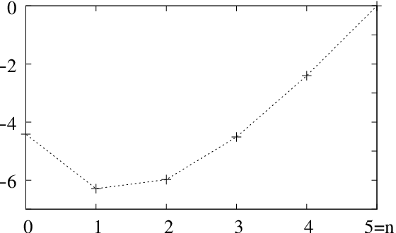
Hence it suffices to show that δ​λk\delta\lambda_{k} is convex with respect to kk, i.e. δ3​λk≥0\delta^{3}\lambda_{k}\geq 0, over {0,…,n−2}\{0,...,n-2\} (see figure 3).

Refer to caption
Figure 3: Graph of δ​λk\delta\lambda_{k} for n=5n=5 (2​n+1=112n+1=11 bodies)

In the above expression of δ3​λk\delta^{3}\lambda_{k}, the denominator is the sine of

0<(2​k+3)​θ4≤2​n−12​n+1⋅π2<π2if0≤k≤n−2,0<(2k+3)\frac{\theta}{4}\leq\frac{2n-1}{2n+1}\cdot\frac{\pi}{2}<\frac{\pi}{2}\quad\mbox{if}\quad 0\leq k\leq n-2,

and thus is >0>0. It remains to check that the numerator

νk=sin⁡((2​k+3)​(n+1)​θ4)​sin⁡((2​k+3)​n​θ4)\nu_{k}=\sin\left((2k+3)(n+1)\frac{\theta}{4}\right)\sin\left((2k+3)n\frac{\theta}{4}\right)

itself is ≥0\geq 0, which follows from linearizing:

νk=12​cos⁡k+32n+12​π2≥0if0≤k≤n−2.\nu_{k}=\frac{1}{2}\cos\frac{k+\frac{3}{2}}{n+\frac{1}{2}}\frac{\pi}{2}\geq 0\quad\mbox{if}\quad 0\leq k\leq n-2.
Case of an even number of bodies: N=2​nN=2n.

In the sum defining λk\lambda_{k}, all terms come pairwise (indexes jj and N−jN-j), except that of the nn-th body. Let ϵj=1/2\epsilon_{j}=1/2 if j=nj=n and ϵj=1\epsilon_{j}=1 otherwise. Then

λk=−14∑j=1nϵj1−cos⁡j​k​θsin3⁡j​θ2(1≤k≤n).\lambda_{k}=-\frac{1}{4}\sum_{j=1}^{n}\epsilon_{j}\frac{1-\cos jk\theta}{\sin^{3}\frac{j\theta}{2}}\quad(1\leq k\leq n).

It follows that

δ​λk=−12∑j=1nϵjsin⁡j⁡(2​k+1)​θ2sin2⁡j​θ2(1≤k≤n−1)δ2​λk=−∑j=1nϵjcos⁡j⁡(k+1)​θsin⁡j​θ2(1≤k≤n−2)δ3​λk=2​∑j=1nϵj​sin⁡j⁡(2​k+3)​θ2(1≤k≤n−3)=2​sin⁡((2​k+3)​(n+1)​θ4)​sin⁡((2​k+3)​n​θ4)sin⁡(2​k+3)​θ4+(−1)k.\begin{array}[t]{rlll}\delta\lambda_{k}&=&-\frac{1}{2}\sum_{j=1}^{n}\epsilon_{j}\frac{\sin j(2k+1)\frac{\theta}{2}}{\sin^{2}j\frac{\theta}{2}}&(1\leq k\leq n-1)\\ \delta^{2}\lambda_{k}&=&-\sum_{j=1}^{n}\epsilon_{j}\frac{\cos j(k+1)\theta}{\sin j\frac{\theta}{2}}&(1\leq k\leq n-2)\\ \delta^{3}\lambda_{k}&=&2\sum_{j=1}^{n}\epsilon_{j}\sin j(2k+3)\frac{\theta}{2}&(1\leq k\leq n-3)\\ &=&2\frac{\sin\left((2k+3)(n+1)\frac{\theta}{4}\right)\sin\left((2k+3)n\frac{\theta}{4}\right)}{\sin(2k+3)\frac{\theta}{4}}+(-1)^{k}.\end{array}

Again, we will check that δ​λk\delta\lambda_{k} is <0<0 at the boundary of some interval of integers containing {1,…,n−1}\{1,...,n-1\}, and that δ​λk\delta\lambda_{k} is convex inside this interval.

Similarly to the odd case, obviously we have δ​λ0<0\delta\lambda_{0}<0 and δ​λn−1/2=0\delta\lambda_{n-1/2}=0. Unfortunately, the latter equality is not of any direct use since the index is not an integer. Let us rather show that

δ​λn−1=12​(∑j=1n(−1)j​ϵjsin2⁡j​π2​n)​sin⁡π2​n\delta\lambda_{n-1}=\frac{1}{2}\left(\sum_{j=1}^{n}\frac{(-1)^{j}\epsilon_{j}}{\sin^{2}j\frac{\pi}{2n}}\right)\sin\frac{\pi}{2n}

is <0<0. It suffices to see that

an=∑j=1n(−1)j​ϵjsin2⁡j​π2​n=∑j=1n−1(−1)jsin2⁡j​π2​n+(−1)n2=∑j=1n(−1)jsin2⁡j​π2​n+(−1)n+12a_{n}=\sum_{j=1}^{n}\frac{(-1)^{j}\epsilon_{j}}{\sin^{2}j\frac{\pi}{2n}}=\sum_{j=1}^{n-1}\frac{(-1)^{j}}{\sin^{2}j\frac{\pi}{2n}}+\frac{(-1)^{n}}{2}=\sum_{j=1}^{n}\frac{(-1)^{j}}{\sin^{2}j\frac{\pi}{2n}}+\frac{(-1)^{n+1}}{2}

is <0<0. Note that in these sums if j≤n−1j\leq n-1 is odd the pair of terms of indices jj and j+1j+1 have a negative contribution. Hence, if nn is odd, the last but one given expression of ana_{n} shows that an≤−1/2a_{n}\leq-1/2; and, if nn is even, the same estimate follows from the last expression.

It remains to show that

δ3​λk=2​sin⁡((2​k+3)​(n+1)​θ4)​sin⁡((2​k+3)​n​θ4)+(−1)k​sin⁡(2​k+3)​θ4sin⁡(2​k+3)​θ4\delta^{3}\lambda_{k}=\frac{2\sin\left((2k+3)(n+1)\frac{\theta}{4}\right)\sin\left((2k+3)n\frac{\theta}{4}\right)+(-1)^{k}\sin(2k+3)\frac{\theta}{4}}{\sin(2k+3)\frac{\theta}{4}}

is positive if 1≤k≤n−21\leq k\leq n-2. The denominator being >0>0, focus on the numerator νk\nu_{k}. Setting α=(k+32)​π2​n\alpha=(k+\frac{3}{2})\frac{\pi}{2n}, we get

νk=2​sin⁡(n+1)​α​sin⁡n​α+(−1)k​sin⁡α;\nu_{k}=2\sin(n+1)\alpha\sin n\alpha+(-1)^{k}\sin\alpha;

splitting (n+1)​α(n+1)\alpha into n​α+αn\alpha+\alpha and partially linearizing yields

cos⁡α⏟>0​((1+cos⁡2​n​α)⏟≥0+tan⁡α​(sin⁡2​n​α+(−1)k)⏟=0)≥0,\underbrace{\cos\alpha}_{>0}\left(\underbrace{(1+\cos 2n\alpha)}_{\geq 0}+\tan\alpha\underbrace{\left(\sin 2n\alpha+(-1)^{k}\right)}_{=0}\right)\geq 0,

which proves the result.

3.3 The symmetry group Gr/s​(N,k,η)G_{r/s}(N,k,\eta)

We will now analyze the symmetries of vertical eigenmodes in the full phase space. Recall that most of the time a vertical eigenfrequency is degenerate and has vertical multiplicity 4. We will let the amplitude and the phase be respectively A=1A=1 and t0=0t_{0}=0, and consider the most symmetric generators of its eigenspace i.e. 22-frequency motions of the form

xj​(t)=(ζj​ei​ω1​t,Re⁡(ζη​k​j​ei​ωk​t))∈ℂ×ℝ,(j=0,⋯,N−1),x_{j}(t)=\left(\zeta^{j}e^{i\omega_{1}t},\mathrm{Re}\,(\zeta^{\eta kj}e^{i\omega_{k}t})\right)\in\mathbb{C}\times\mathbb{R},\quad(j=0,\cdots,N-1), S⁡(N,k,η)

where η=±1\eta=\pm 1 and, like in the former section, ζ=ei​2​πN\zeta=e^{i\frac{2\pi}{N}} and k∈{1,…​n}k\in\{1,...n\}. When observed in a frame rotating around the vertical axis with angular velocity ϖ\varpi such that

ω1−ϖωk=rs∈ℚ,\frac{\omega_{1}-\varpi}{\omega_{k}}=\frac{r}{s}\in\mathbb{Q},

the horizontal and vertical frequencies are set into resonance and the motion becomes periodic of period T=2​π​sωkT=\frac{2\pi s}{\omega_{k}}:

xj​(t)=(ζj​ei​rs​ωk​t,Re⁡(ζη​k​j​ei​ωk​t))(j=0,…,N−1)x_{j}(t)=\left(\zeta^{j}e^{i\frac{r}{s}\omega_{k}t},\mathrm{Re}\,(\zeta^{\eta kj}e^{i\omega_{k}t})\right)\quad(j=0,...,N-1) Sr/s​(N,k,η).

The discrete symmetry group of such a motion is seeked as before as a subgroup of

G0=O⁡(ℝ/T​ℤ)×Σ⁡(N)×O⁡(ℝ3),G_{0}=O(\mathbb{R}/T\mathbb{Z})\times\Sigma(N)\times O(\mathbb{R}^{3}),

where g=(τ,σ,ρ)∈G0g=(\tau,\sigma,\rho)\in G_{0} acts naturally on the space of TT-periodic loops: g​xj​(t)=ρ​xσ−1​(j)​(τ−1​(t))gx_{j}(t)=\rho x_{\sigma^{-1}(j)}(\tau^{-1}(t)).

Let Gr/s​(N,k,η)G_{r/s}(N,k,\eta) be the stabilizer of Sr/s​(N,k,η)S_{r/s}(N,k,\eta). The group structure of Gr/s​(N,k,η)G_{r/s}(N,k,\eta) does not depend on rr and it depends on ss only through the fact that we are looking to the solution during a time interval ss times longer than the minimal period of the relative equilibrium in the inertial frame. We let (s,k)(s,k) be the gcd of ss and kk, and s=(s,k)​s′,k=(s,k)​k′s=(s,k)s^{\prime},\;k=(s,k)k^{\prime}.

Lemma 12

Gr/s​(N,k,η)G_{r/s}(N,k,\eta) is a semi-direct product of an Abelian group HH of order 2​N​s2Ns by ℤ/2​ℤ\mathbb{Z}/2\mathbb{Z}. The group HH is an extension by ℤ/2​ℤ\mathbb{Z}/2\mathbb{Z} of a group KK which is itself an extension of ℤ/N​s′​ℤ\mathbb{Z}/Ns^{\prime}\mathbb{Z} by ℤ/(k,s)​ℤ\mathbb{Z}/(k,s)\mathbb{Z}.

Proof.

  • 1io

    Restriction to a subgroup G1G_{1} of G0G_{0}. Certainly elements of Gr/s​(N,k,η)G_{r/s}(N,k,\eta) stabilize the regular NN-gon relative equilibrium (as the horizontal component of any infinitesimal vertical variations), as well as the cylinder of infinitesimal vertical variations. Hence Gr/s​(N,k,η)G_{r/s}(N,k,\eta) is contained in the subgroup G1G_{1} consisting of elements g=(τ,σ,ρ)∈G0g=(\tau,\sigma,\rho)\in G_{0} satisfying the following conditions:

    • —

      The isometry ρ∈O⁡(ℝ3)\rho\in O(\mathbb{R}^{3}) is of the form ρ=(ρh​o​r,ρv​e​r):ℂ×ℝ↦ℂ×ℝ\rho=(\rho_{hor},\rho_{ver}):\mathbb{C}\times\mathbb{R}\mapsto\mathbb{C}\times\mathbb{R} where

      ρh​o​r​(h)=ei​2​π​α​horei​2​π​α​h¯andρv​e​r​(v)=ei​π​β​v\rho_{hor}(h)=e^{i2\pi\alpha}h\quad\mbox{or}\quad e^{i2\pi\alpha}\bar{h}\quad\mbox{and}\quad\rho_{ver}(v)=e^{i\pi\beta}v

      with α∈ℝ/ℤ\alpha\in\mathbb{R}/\mathbb{Z} and β∈ℤ/2​ℤ\beta\in\mathbb{Z}/2\mathbb{Z}.

    • —

      If we set ξ=±1\xi=\pm 1 according to whether ρh​o​r​(h)=ei​2​π​α​h\rho_{hor}(h)=e^{i2\pi\alpha}h or ei​2​π​α​h¯e^{i2\pi\alpha}\bar{h}, τ−1​(t)=ξ⁡(t−θ)\tau^{-1}(t)=\xi(t-\theta) with θ∈ℝ/T​ℤ\theta\in\mathbb{R}/T\mathbb{Z}.

    Hence an element g∈G1g\in G_{1} can be identified with a quintuple

    (θ,σ,α,β,ξ)∈ℝ/T​ℤ×Σ⁡(N)×ℝ/ℤ×ℤ/2​ℤ×𝔽2,(\theta,\sigma,\alpha,\beta,\xi)\in\mathbb{R}/T\mathbb{Z}\times\Sigma(N)\times\mathbb{R}/\mathbb{Z}\times\mathbb{Z}/2\mathbb{Z}\times\mathbb{F}_{2},

    the multiplication law being given by g~=g′​g\tilde{g}=g^{\prime}g with

    θ~=θ′+ξ′​θ,σ~=σ′​σ,α~=α′+ξ′​α,β~=β′+β,ξ~=ξ′​ξ.\tilde{\theta}=\theta^{\prime}+\xi^{\prime}\theta,\;\tilde{\sigma}=\sigma^{\prime}\sigma,\;\tilde{\alpha}=\alpha^{\prime}+\xi^{\prime}\alpha,\;\tilde{\beta}=\beta^{\prime}+\beta,\;\tilde{\xi}=\xi^{\prime}\xi.

    In the rest of this proof, let us set the time unit so that ωk=2​π\omega_{k}=2\pi, i.e. T=sT=s: if x∈Sr/s​(N,k,η)x\in S_{r/s}(N,k,\eta),

    g​xj=(exp⁡(2​π​i​[α+1N​ξ​σ−1​(j)+rs​(t−θ)])cos⁡(2​π​[β2+ηN​k​σ−1​(j)+ξ⁡(t−θ)])).gx_{j}=\left(\begin{array}[c]{l}\exp\left(2\pi i\left[\alpha+\frac{1}{N}\xi\sigma^{-1}(j)+\frac{r}{s}(t-\theta)\right]\right)\\ \cos\left(2\pi\left[\frac{\beta}{2}+\frac{\eta}{N}k\sigma^{-1}(j)+\xi(t-\theta)\right]\right)\end{array}\right).
  • 2io

    Restriction to a subgroup G2G_{2} of G1G_{1}. Setting δ=ξ​σ−1​(j)−j∈ℤ/N​ℤ\delta=\xi\sigma^{-1}(j)-j\in\mathbb{Z}/N\mathbb{Z}, the symmetry equation g​x=xgx=x reduces to

    {α+δN−rs​θ≡0(mod1)ξ​β2+k​η​δN−θ≡0(mod1).\left\{\begin{array}[c]{l}\alpha+\frac{\delta}{N}-\frac{r}{s}\theta\equiv 0\;\pmod{1}\\ \xi\frac{\beta}{2}+k\eta\frac{\delta}{N}-\theta\equiv 0\;\pmod{1}.\end{array}\right.

    The first equation shows that δ\delta is independent of jj, i.e. ξ​σ\xi\sigma is a circular permutation. Hence, using the fact that ξ​β=β(mod1)\xi\beta=\beta\pmod{1},

    {α≡rsθ−δN(mod1)θ≡β2+kηδN(mod1)\left\{\begin{array}[c]{l}\alpha\equiv\frac{r}{s}\theta-\frac{\delta}{N}\quad\pmod{1}\\ \theta\equiv\frac{\beta}{2}+k\eta\frac{\delta}{N}\quad\pmod{1}\end{array}\right.

    These equations completely determine α∈ℝ/ℤ\alpha\in\mathbb{R}/\mathbb{Z} as a function of δ\delta and θ\theta but θ∈ℝ/s​ℤ\theta\in\mathbb{R}/s\mathbb{Z} is only determined mod 1, as a function of (δ,β,ξ)∈ℤN×ℤ/2​ℤ×𝔽2(\delta,\beta,\xi)\in\mathbb{Z}_{N}\times\mathbb{Z}/2\mathbb{Z}\times\mathbb{F}_{2}. Let

    G2=(ℝ/s​ℤ×ℤ/N​ℤ×ℤ/2​ℤ)⋊𝔽2={(θ,δ,β,ξ)},G_{2}=(\mathbb{R}/s\mathbb{Z}\times\mathbb{Z}/N\mathbb{Z}\times\mathbb{Z}/2\mathbb{Z})\rtimes\mathbb{F}_{2}=\{(\theta,\delta,\beta,\xi)\},

    where the semi-direct product is defined by the law g~=g′​g\tilde{g}=g^{\prime}g, with

    θ~=θ′+ξ′​θ,δ~=δ′+ξ′​δ,β~=β′+β,ξ~=ξ′​ξ.\tilde{\theta}=\theta^{\prime}+\xi^{\prime}\theta,\;\tilde{\delta}=\delta^{\prime}+\xi^{\prime}\delta,\;\tilde{\beta}=\beta^{\prime}+\beta,\;\tilde{\xi}=\xi^{\prime}\xi.

    Then Gr/s​(N,k,η)G_{r/s}(N,k,\eta) identifies with the subgroup of G2G_{2} defined by the equation

    θ≡β2+k​η​δN(mod1).\theta\equiv\frac{\beta}{2}+k\eta\frac{\delta}{N}\pmod{1}.
  • 3io

    Group structure of Gr/s​(N,k,η)G_{r/s}(N,k,\eta).

    (i) The semi-direct product structure of G2G_{2} goes down to Gr/s​(N,k,η)G_{r/s}(N,k,\eta). Indeed, the section ξ↦(0,0,0,ξ)\xi\mapsto(0,0,0,\xi) of the projection G2→𝔽2G_{2}\to\mathbb{F}_{2} takes its values in the subgroup Gr/s​(N,k,η)G_{r/s}(N,k,\eta). Hence Gr/s​(N,k,η)=H⋊ℤ/2​ℤG_{r/s}(N,k,\eta)=H\rtimes\mathbb{Z}/2\mathbb{Z}, where HH is the subgroup of the abelian group ℝ/s​ℤ×ℤ/N​ℤ×ℤ/2​ℤ\mathbb{R}/s\mathbb{Z}\times\mathbb{Z}/N\mathbb{Z}\times\mathbb{Z}/2\mathbb{Z} defined as the set of triples (θ,δ,β)(\theta,\delta,\beta) which satisfy

    θ≡β2+k​η​δN(mod1).\theta\equiv\frac{\beta}{2}+k\eta\frac{\delta}{N}\pmod{1}.

    (ii) Let KK be the kernel of the group homomorphism (θ,δ,β)↦β(\theta,\delta,\beta)\mapsto\beta from HH to ℤ/2​ℤ\mathbb{Z}/2\mathbb{Z}. It can be identified with the subgroup of ℝ/s​ℤ×ℤ/N​ℤ\mathbb{R}/s\mathbb{Z}\times\mathbb{Z}/N\mathbb{Z} defined as the set of pairs (θ,δ)(\theta,\delta) which satisfy

    θ≡k​η​δN(mod1).\theta\equiv k\eta\frac{\delta}{N}\pmod{1}.

    (iii) One has the exact sequence

    0→ℤ/N​s′​ℤ→K→ℤ/(k,s)​ℤ→0,0\rightarrow\mathbb{Z}/Ns^{\prime}\mathbb{Z}\rightarrow K\rightarrow\mathbb{Z}/(k,s)\mathbb{Z}\rightarrow 0,

    where the first arrow sends 1 to (k​η/N,1)(k\eta/N,1) and the second one sends (θ,δ)(\theta,\delta) to the class of θ−k​η​δ/N\theta-k\eta\delta/N. This ends the proof of the lemma.

The precise structure of Gr/s​(N,k,η)G_{r/s}(N,k,\eta) depends on s,N,k,ηs,N,k,\eta. We study it in some cases.

Lemma 13

If one of the following conditions is satisfied, HH is isomorphic to K×ℤ/2​ZK\times\mathbb{Z}/2Z:

1) ss is odd

2) ss and NN are even, kk is odd.

Proof.

1) If ss is odd, the mapping β↦(s​β2,0,β)\beta\mapsto(\frac{s\beta}{2},0,\beta) defines a section of the projection from HH to ℤ/2​ℤ\mathbb{Z}/2\mathbb{Z}. Hence the mapping (θ,δ,β)↦((θ−s​β2,δ),β)(\theta,\delta,\beta)\mapsto\bigl((\theta-\frac{s\beta}{2},\delta),\beta\bigr) is an isomorphism from HH to K×ℤ/2​ℤK\times\mathbb{Z}/2\mathbb{Z}.

2) If s=2​σs=2\sigma is even, a section must send 1 onto an element of order 2 in HH not belonging to KK, i.e. an element of the form (θ,δ,1)(\theta,\delta,1) such that there exist a,b∈ℤa,b\in\mathbb{Z} with

2​δ=b​N,1+2​k​η​δN=1+b​k​η=a​s=2​a​σ.2\delta=bN,\quad\quad 1+2k\eta\frac{\delta}{N}=1+bk\eta=as=2a\sigma.

From the second equation, it follows that bb and kk must be odd. The first one then implies that NN is even. If all these conditions are satisfied, β↦(β​s2,β​N2,β)\beta\mapsto(\beta\frac{s}{2},\beta\frac{N}{2},\beta) defines a section and hence the mapping (θ,δ,β)↦((θ−β​s2,δ−β​N2),β)(\theta,\delta,\beta)\mapsto\bigl((\theta-\beta\frac{s}{2},\delta-\beta\frac{N}{2}),\beta\bigr) is an isomorphism from HH to K×ℤ/2​ℤK\times\mathbb{Z}/2\mathbb{Z}.

Lemma 14

If (k,s′)=1(k,s^{\prime})=1, KK is isomorphic to ℤ/N​s′​ℤ×ℤ/(k,s)​ℤ\mathbb{Z}/Ns^{\prime}\mathbb{Z}\times\mathbb{Z}/(k,s)\mathbb{Z} (and hence to ℤ/N​s​ℤ\mathbb{Z}/Ns\mathbb{Z} if (N​s′,(k,s))=1(Ns^{\prime},(k,s))=1); if (N​k′,(k,s))=1(Nk^{\prime},(k,s))=1, KK is isomorphic to ℤ/N​s​ℤ\mathbb{Z}/Ns\mathbb{Z}.

1) If (k,s′)=1(k,s^{\prime})=1, the mapping which sends 1∈ℤ/(k,s)​ℤ1\in\mathbb{Z}/(k,s)\mathbb{Z} to (s′,0)∈K(s^{\prime},0)\in K is a section.

2) If (N​k′,(k,s))=1(Nk^{\prime},(k,s))=1, this implies (N,(k,s))=1(N,(k,s))=1, and hence the existence of integers l′l^{\prime} and δ\delta such that N​l′+η​δ​(k,s)=1Nl^{\prime}+\eta\delta(k,s)=1. Let us set l=l′​k′l=l^{\prime}k^{\prime} and θ=k​η​δ/N+l\theta=k\eta\delta/N+l. We assert that the element (θ,δ)(\theta,\delta) is of order N​sNs. Indeed, p⁡(θ,δ)=0∈Kp(\theta,\delta)=0\in K if and only if there exists integers a,ba,b such that

p​k​η​δ/N+p​l=k​η​b+p​l=a​s,p​δ=b​N.pk\eta\delta/N+pl=k\eta b+pl=as,\quad p\delta=bN.

From its definition δ\delta satisfies (N,δ)=1(N,\delta)=1. Then, the second equation above implies the existence of an integer p′p^{\prime} such that p=p′​Np=p^{\prime}N, hence b=p′​δb=p^{\prime}\delta and the first equation above becomes p′​((k,s)​η​δ+N​l′)​k′=a​sp^{\prime}\bigl((k,s)\eta\delta+Nl^{\prime}\bigr)k^{\prime}=as, that is p′​k′=a​sp^{\prime}k^{\prime}=as. As (N​k′,(k,s))=1(Nk^{\prime},(k,s))=1 implies (k′,(k,s))=1(k^{\prime},(k,s))=1 and hence (k′,s)=1(k^{\prime},s)=1, there exists an integer p′′p^{\prime\prime} such that p′=p′′​sp^{\prime}=p^{\prime\prime}s, and hence that p=p′′​N​sp=p^{\prime\prime}Ns.

Corollary 15

When s=1s=1, Gr/s​(N,k,η)G_{r/s}(N,k,\eta) is isomorphic to the direct product DN×ℤ/2​ℤD_{N}\times\mathbb{Z}/2\mathbb{Z}, where DND_{N}, of order 2​N2N, is the dihedral group. In particular, when NN is odd, it is isomorphic to D2​ND_{2N}.

3.4 Invariant loops

An ss-periodic loop of configurations x⁡(t)=(x1​(t),⋯,xN​(t))x(t)=\bigl(x_{1}(t),\cdots,x_{N}(t)\bigr) is invariant under the action of Gr/s​(N,k,η)G_{r/s}(N,k,\eta) if and only if, for every (θ,δ,β,ξ)∈G2(\theta,\delta,\beta,\xi)\in G_{2} representing an element of Gr/s​(N,k,η)G_{r/s}(N,k,\eta), i.e. such that θ−β2−k​η​δN=l∈ℤ\theta-\frac{\beta}{2}-k\eta\frac{\delta}{N}=l\in\mathbb{Z}, one has

∀j∈ℤ/N​ℤ,xj​(t)=ρ​xξ⁡(j+δ)​(ξ⁡(t−θ)),\forall j\in\mathbb{Z}/{N\mathbb{Z}},\;x_{j}(t)=\rho x_{\xi(j+\delta)}\bigl(\xi(t-\theta)\bigr),

where the action of ρ\rho on ℝ3=ℂ×ℝ\mathbb{R}^{3}=\mathbb{C}\times\mathbb{R} is defined by

ρ⁡(h,z)=(ei​2​π​α​h¯ξ,ei​π​β​z)withα=rs​θ−δN(mod1),\rho(h,z)=(e^{i2\pi\alpha}\bar{h}^{\xi},e^{i\pi\beta}z)\quad\mbox{with}\quad\alpha=\frac{r}{s}\theta-\frac{\delta}{N}\pmod{1},

where h¯ξ=h\bar{h}^{\xi}=h if ξ=+1\xi=+1 and h¯ξ=h¯\bar{h}^{\xi}=\bar{h} if ξ=−1\xi=-1.

Before looking at remarkable classes of invariant loops, let us make some general comments:

1. Taking (θ=12+l,δ=0,β=1,ξ=1)(\theta=\frac{1}{2}+l,\delta=0,\beta=1,\xi=1) and setting xj​(t)=(hj​(t),zj​(t))x_{j}(t)=(h_{j}(t),z_{j}(t)), we get

hj​(t)=ei​2​π​rs​(12+l)​hj​(t−12+l),zj​(t)=−zj​(t−12+l).h_{j}(t)=e^{i2\pi\frac{r}{s}(\frac{1}{2}+l)}h_{j}(t-\frac{1}{2}+l),\quad z_{j}(t)=-z_{j}(t-\frac{1}{2}+l).

In particular, if s=2​l+1s=2l+1 and rr are odd, an invariant loop possesses the Italian symmetry. This is the case of the Hip-Hops and of chains with an odd number of lobes (see below).

2. Taking (θ=0,δ=0,β=0,ξ=−1)(\theta=0,\delta=0,\beta=0,\xi=-1), we get

hj​(t)=h¯−j​(−t),zj​(t)=z−j​(−t).h_{j}(t)=\bar{h}_{-j}(-t),\quad z_{j}(t)=z_{-j}(-t).

In particular, when t=0t=0, the configuration is always symmetric with respect to the vertical plane containing the first coordinate axis.

3. Taking (θ=k​ηN,δ=1,β=0,ξ=1)(\theta=\frac{k\eta}{N},\delta=1,\beta=0,\xi=1), we get

hj​(t)=ei​2​π​AN​hj+1​(t−k​ηN),zj​(t)=zj+1​(t−k​ηN).h_{j}(t)=e^{i2\pi\frac{A}{N}}h_{j+1}(t-\frac{k\eta}{N}),\quad z_{j}(t)=z_{j+1}(t-\frac{k\eta}{N}).

where A=rs​k​η−1A=\frac{r}{s}k\eta-1.

More generally, the smallest non zero value of θ=β2+k​η​δN+l=N⁡(β+2​l)+2​k​η​δ2​N\theta=\frac{\beta}{2}+k\eta\frac{\delta}{N}+l=\frac{N(\beta+2l)+2k\eta\delta}{2N} is θ0=(N,2​k)2​N\theta_{0}=\frac{(N,2k)}{2N} because β+2​l\beta+2l and δ\delta are arbitrary integers.

One can distinguish two cases in the action of Gr/s​(N,k,η)G_{r/s}(N,k,\eta) on the space of loops of NN-body configurations. In the first one, exemplified by the P12P_{12} family for 3 bodies, no a priori spatial symmetry of the configuration exists for all times, and even α=0\alpha=0 for any element of the group. In this case, the group acts on the full space of similitude classes of NN-body configurations. The condition is that for any l∈ℤ,δ∈ℤ/ℕ​ℤ,β∈ℤ,l\in\mathbb{Z},\,\delta\in\mathbb{Z}/\mathbb{N}\mathbb{Z},\,\beta\in\mathbb{Z}, rs​[β2+k​η​δN+l]−δN=0(mod1).\frac{r}{s}\bigl[\frac{\beta}{2}+k\eta\frac{\delta}{N}+l\bigr]-\frac{\delta}{N}=0\;\pmod{1}. This is equivalent to s=1,r=2​r′, 2​r′​k​η−1=0(modN)s=1,\,r=2r^{\prime},\,2r^{\prime}k\eta-1=0\pmod{N} (which implies that NN is odd). The case rs=2​r′=N−1,k=1,η=−1\frac{r}{s}=2r^{\prime}=N-1,k=1,\eta=-1 corresponds to the “unchained polygons” with N−1N-1 lobes.

In the second one, exemplified by the Hip-Hop family for 4 bodies, such a symmetry does exist: there is a group element such that θ=0,δ=−1,α=1/N\theta=0,\,\delta=-1,\,\alpha=1/N. In this case, the group acts on a subspace of the space of similitude classes of NN-body configurations. The condition is that β2−k​ηN=0(mod1)\frac{\beta}{2}-\frac{k\eta}{N}=0\pmod{1} which, because k≤N2k\leq\frac{N}{2}) implies β=1\beta=1 and k​η=N2k\eta=\frac{N}{2} (the choice of η=±1\eta=\pm 1 is then immaterial because ek​2​πN=e−k​2​πNe^{k\frac{2\pi}{N}}=e^{-k\frac{2\pi}{N}}, so we set η=1\eta=1). The N=2​N′N=2N^{\prime}-body Hip-Hops studied in [TV, BCPS] fall into this category; the group element is (θ=0,δ=−1,ξ=1,α=1N)(\theta=0,\delta=-1,\xi=1,\alpha=\frac{1}{N}), which sends one body onto the next one by a rotation of 2​πN\frac{2\pi}{N} followed by a change of sign in the vertical component. We now study some types of symmetric loops in the two cases.

The choreographic symmetry

(bodies gather by pairs, at least, following the same curve in space): this corresponds to a group element gg with ξ=1,δ≠0,α=0,β=0\xi=1,\delta\neq 0,\alpha=0,\beta=0. The equations defining the symmetry group become

{δN−rs​θ≡0(mod1)k​η​δN−θ≡0(mod1).\left\{\begin{array}[c]{l}\frac{\delta}{N}-\frac{r}{s}\theta\equiv 0\;\pmod{1}\\ k\eta\frac{\delta}{N}-\theta\equiv 0\;\pmod{1}.\end{array}\right.

Choreographies can be simple or multiple. They are simple if all the bodies lie on the same curve, i.e. if in addition σ\sigma has a unique cycle:

(δ,N)=1.(\delta,N)=1.
Lemma 16

Sr/s​(N,k,η)S_{r/s}(N,k,\eta) is a simple choreography if and only if

s−k​η​r=0(modN).s-k\eta r=0\;\pmod{N}.

Proof. We rewrite more explicitely the conditions for being a choreography: there exists integers l,ml,m such that

{s​δ−N​r​θ=l​s​Nk​η​δ−N​θ=m​N.\left\{\begin{array}[c]{l}s\delta-Nr\theta=lsN\\ k\eta\delta-N\theta=mN.\end{array}\right.

This is equivalent to

{(s−k​η​r)​δ=(l​s−m​r)​Nk​η​δ−N​θ=m​N.\left\{\begin{array}[c]{l}(s-k\eta r)\delta=(ls-mr)N\\ k\eta\delta-N\theta=mN.\end{array}\right.

Due to the condition of simple choreography (δ,N)=1(\delta,N)=1, this is equivalent to the existence of an integer aa such that

{l​s−m​r=a​δs−k​η​r=a​Nk​η​δ−N​θ=m​N.\left\{\begin{array}[c]{l}ls-mr=a\delta\\ s-k\eta r=aN\\ k\eta\delta-N\theta=mN.\end{array}\right.

This proves the “only if” part of the lemma.

For the “if” part, let us suppose that there exists an integer aa such that s−k​η​r=a​Ns-k\eta r=aN. As (r,s)=1(r,s)=1, we can choose l,ml,m such that l​s+m​r=als+mr=a. We then define

g=(θ=k​ηN−m,δ=1,ξ=1,α=0,β=0)∈Gr/s​(N,k,η),g=\left(\theta=\frac{k\eta}{N}-m,\delta=1,\xi=1,\alpha=0,\beta=0\right)\in G_{r/s}(N,k,\eta),

which completes the proof.

Remark

The condition of simple choreography could of course have been obtained directly from the formulae for invariant loops or by writing that for all jj, one has (ζη​k​j​ei​ωk​t)rs=ζj​ei​rs​ωk​t\bigl(\zeta^{\eta kj}e^{i\omega_{k}t}\bigr)^{\frac{r}{s}}=\zeta^{j}e^{i\frac{r}{s}\omega_{k}t}, which expresses that all the bodies belong to the curve described by the first.

Corollary 17

For any N,k,ηN,k,\eta, the set of values of r/sr/s for which Sr/s​(N,k,η)S_{r/s}(N,k,\eta) is a simple choreography is dense in ℝ\mathbb{R}.

Proof. The integers N,k,ηN,k,\eta being given, r,s,ar,s,a must be such that

(r,s)=1ands−k​η​r=a​N.(r,s)=1\quad\hbox{and}\quad s-k\eta r=aN.

The primality condition is equivalent to the existence of integers l,ml,m such that l​s+m​r=1ls+mr=1 , that is (m+l​k​η)​r+l⁡(a​N)=1(m+lk\eta)r+l(aN)=1. As (m+l​k​η,l)(m+lk\eta,l) can be an arbitrary pair of integers, this is equivalent to (r,a​N)=1(r,aN)=1. But the density of the r/sr/s is equivalent to the density of s/r=k​η+a​N/rs/r=k\eta+aN/r and hence to the density of the a​N/raN/r or equivalently of the r/a​Nr/aN, with the unique condition that (r,a​N)=1(r,aN)=1. As the irreducible fractions of the form r/Nir/N^{i} are dense, the corollary follows.

Eights and maximal chains symmetries

The two choreographic cases with extreme values of kk are G2​(N=2​n+1,n,−1)G_{2}(N=2n+1,n,-1) (which we call the Eight symmetry) and GN−1​(N,1,−1)G_{N-1}(N,1,-1) (resp. the maximal chain symmetry). In the first case, the group element (θ=12​N,δ=1,β=1,ξ=1)(\theta=\frac{1}{2N},\delta=1,\,\beta=1,\,\xi=1) leads to

xj​(t)=xj+1​(t−12​N),zj​(t)=−zj+1​(t−12​N);x_{j}(t)=x_{j+1}(t-\frac{1}{2N}),\;z_{j}(t)=-z_{j+1}(t-\frac{1}{2N});

in the second case, the group element (θ=12​N,δ=n,β=1,ξ=1)(\theta=\frac{1}{2N},\delta=n,\,\beta=1,\,\xi=1) leads to

xj​(t)=xj+n​(t−12​N),zj​(t)=−zj+n​(t−12​N).x_{j}(t)=x_{j+n}(t-\frac{1}{2N}),\;z_{j}(t)=-z_{j+n}(t-\frac{1}{2N}).

Solutions invariant under such a symmetry are called unchained polygons because the horizontal rotation of the regular NN-gon is unfolded in the vertical direction, into a choreographic chain with 2 and N−1N-1 lobes respectively. Examples are shown on figures 4.2 and 4.1.

The Hip-Hop symmetry

Writing k=(N,k)​k~,N=(N,k)​N~k=(N,k)\tilde{k},\,N=(N,k)\tilde{N}, we notice that

ζη​k​j1=ζη​k​j2if and only ifj2−j1is a multiple of N~.\zeta^{\eta kj_{1}}=\zeta^{\eta kj_{2}}\quad\hbox{if and only if}\quad j_{2}-j_{1}\quad\hbox{is a multiple of }\;\tilde{N}.

Hence the bodies are divided into N~\tilde{N} regular (N,k)(N,k)-gons which remain horizontal at each instant. Independantly of the chosen rotating frame, the motion is invariant under a group element gg of the form

g=(θ=0,δ=N~,α=−1(N,k),β=0)∈G1,1​(N,k,η).g=\left(\theta=0,\,\delta=\tilde{N},\,\alpha=-\frac{1}{(N,k)},\,\beta=0\right)\in G_{1,1}(N,k,\eta).

If we make the simplest possible choice r/s=1r/s=1, we get a Hip-Hop motion. The name is a reference to the original Hip-Hop solution where the two diagonals of a square stay horizontal while undergoing vertical oscillations (see figure 4.6). Note that this symmetry can be combined with a choreographic symmetry.

A few examples of Lyapunov cylinders are shown on figure 4. They are respectively tangent at the relative equilibrium to the following Lyapunov families (the terminology will be explained in section 5):

1. S4​(5,1,−1)S_{4}(5,1,-1) Maximal unchained polygon (ℓ=4\ell=4)
2. S2​(5,2,−1)S_{2}(5,2,-1) Five-body Eight
3. S3​(4,1,−1)S_{3}(4,1,-1) Unchained polygon (Gerver family)
4. S3/2​(4,2,1)S_{3/2}(4,2,1) Terracini-Venturelli choreography (Hip-Hop family)
5. S1​(6,1,−1)S_{1}(6,1,-1) Six-body Hip-Hop
6. S2​(6,2,1)S_{2}(6,2,1) Yet another six-body Hip-Hop.
Refer to caption
Figure 4: Some examples of first order solutions having special symmetries in a resonant rotating frame.

3.5 Isomorphic symmetries

In order to better understand minimizers of the Lagrangian action among loops which in the rotating frame are invariant under the Gr/s​(N,k,η)G_{r/s}(N,k,\eta) action described above, we study the cases when the actions of two groups Gr/s​(N,k,η)G_{r/s}(N,k,\eta) and Gr′/s′​(N,k′,η′)G_{r^{\prime}/s^{\prime}}(N,k^{\prime},\eta^{\prime}) coincide up to a relabelling j↦j′=Σ⁡(j)j\mapsto j^{\prime}=\Sigma(j) of the bodies. A first condition is that the periods coincide, i.e. s′=ss^{\prime}=s.

We will stick for simplicity to the case s=s′=1s=s^{\prime}=1.

Let as usual ζ=e2​π​i/N\zeta=e^{2\pi i/N}; the horizontal relative equilibrium whose j′j^{\prime}th body’s motion is hj′′​(t)=ζj′​e2​π​i​r′​th^{\prime}_{j^{\prime}}(t)=\zeta^{j^{\prime}}e^{2\pi ir^{\prime}t} is Gr′​(N,k′,η′)G_{r^{\prime}}(N,k^{\prime},\eta^{\prime})-symmetric. Hence a necessary condition for the two actions to coincide up to the relabelling Σ\Sigma is that the horizontal relative equilibrium whose jjth body’s motion is

hj​(t)=hΣ⁡(j)′​(t)=ζΣ⁡(j)​e2​π​i​r′​th_{j}(t)=h^{\prime}_{\Sigma(j)}(t)=\zeta^{\Sigma(j)}e^{2\pi ir^{\prime}t}

be Gr​(N,k,η)G_{r}(N,k,\eta)-symmetric. This means that for any (δ,β,ξ)∈Gr​(N,k,η)(\delta,\beta,\xi)\in G_{r}(N,k,\eta),

e2​π​i​α​ζξ​Σ​(ξ⁡(j+δ))​e2​π​i​r′​ξ2​(t−θ)=ζΣ⁡(j)​e2​π​i​r′​t.e^{2\pi i\alpha}\zeta^{\xi\Sigma(\xi(j+\delta))}e^{2\pi ir^{\prime}\xi^{2}(t-\theta)}=\zeta^{\Sigma(j)}e^{2\pi ir^{\prime}t}.

Using the identities θ=β2+k​η​δN(mod1)\theta=\frac{\beta}{2}+k\eta\frac{\delta}{N}\pmod{1} and α=rs​θ−δN(mod1)\alpha=\frac{r}{s}\theta-\frac{\delta}{N}\pmod{1}, this becomes

(r−r′)​[β2+k​η​δN]−δN+1N​[ξ​Σ​(ξ⁡(j+δ))−Σ⁡(j)]=0(mod1).(r-r^{\prime})\bigl[\frac{\beta}{2}+k\eta\frac{\delta}{N}\bigr]-\frac{\delta}{N}+\frac{1}{N}\bigl[\xi\Sigma(\xi(j+\delta))-\Sigma(j)\bigr]=0\pmod{1}.

δ=0,β=1,ξ=1\delta=0,\beta=1,\xi=1, we get a first necessary condition

1)r−r′=2​p∈2​ℤ.\mbox{1)}\quad r-r^{\prime}=2p\in 2\mathbb{Z}.

Taking then δ=0,β=0\delta=0,\beta=0, we get ξ​Σ​(ξ​j)=Σ⁡(j)(modN)\xi\Sigma(\xi j)=\Sigma(j)\pmod{N}. In particular, if ξ=−1\xi=-1 and j=0j=0 we get Σ⁡(0)=0(modN)\Sigma(0)=0\pmod{N}. Finally, taking δ=1,β=0\delta=1,\beta=0, we get Σ⁡(j+1)−Σ⁡(j)=1−2​p​k​η(modN)\Sigma(j+1)-\Sigma(j)=1-2pk\eta\pmod{N}, hence Σ⁡(j)=(1−2​p​k​η)​j(modN)\Sigma(j)=(1-2pk\eta)j\pmod{N}. Interchanging the roles of the two groups we see that necessarily Σ−1​(j′)=(1+2​p​k′​η′)​j′(modN)\Sigma^{-1}(j^{\prime})=(1+2pk^{\prime}\eta^{\prime})j^{\prime}\pmod{N}. This yields a second necessary condition

2)(1−2​p​k​η)​(1+2​p​k​η′)=1(modN).\mbox{2)}\quad(1-2pk\eta)(1+2pk\eta^{\prime})=1\pmod{N}.

It turns out that these necessary conditions are essentially sufficient. Indeed, it is enough to replace the condition 2), which can be written −2​p​[−k​η+k′​η′−2​p​k​η​k′​η′]=0(modN)-2p[-k\eta+k^{\prime}\eta^{\prime}-2pk\eta k^{\prime}\eta^{\prime}]=0\pmod{N} by the slightly stronger condition 2’) below:

Proposition 18

A necessary and sufficient condition for the existence of a permutation 𝔖\mathfrak{S} of ℤ/N​ℤ\mathbb{Z}/N\mathbb{Z} such that for any Gr′​(N,k′,η′)G_{r^{\prime}}(N,k^{\prime},\eta^{\prime})-invariant loop x′​(t)x^{\prime}(t) whose j′j^{\prime}th body motion is (hj′′​(t),zj′′​(t))(h^{\prime}_{j^{\prime}}(t),z^{\prime}_{j^{\prime}}(t)), the loop x⁡(t)x(t) whose jjth body motion is (hj​(t),zj​(t)):=(h𝔖⁡(j)′​(t),z𝔖⁡(j)′​(t))(h_{j}(t),z_{j}(t)):=\bigl(h^{\prime}_{\mathfrak{S}(j)}(t),z^{\prime}_{\mathfrak{S}(j)}(t)\bigr) be Gr​(N,k,η)G_{r}(N,k,\eta)-invariant is that the following conditions be satisfied:

1) r−r′=2​p∈2​ℤr-r^{\prime}=2p\in 2\mathbb{Z},

2’) −k​η+k′​η′−2​p​k​η​k′​η′=0(modN)-k\eta+k^{\prime}\eta^{\prime}-2pk\eta k^{\prime}\eta^{\prime}=0\pmod{N}.

The permutation 𝔖\mathfrak{S} and its inverse are then respectively j↦j′=(1−2​p​k​η)​jj\mapsto j^{\prime}=(1-2pk\eta)j and j′↦j=(1+2​p​k′​η′)​j′j^{\prime}\mapsto j=(1+2pk^{\prime}\eta^{\prime})j^{\prime} in ℤ/N​ℤ\mathbb{Z}/N\mathbb{Z}.

Proof. We already know that the asserted form of the permutation 𝔖\mathfrak{S} is necessary. What remains is a direct computation: in order to show the invariance of the loop x⁡(t)x(t) under the element of Gr​(N,k,η)G_{r}(N,k,\eta) represented by (δ,β,ξ)(\delta,\beta,\xi), one must find an element of Gr′​(N,k′,η′)G_{r^{\prime}}(N,k^{\prime},\eta^{\prime}) repesented by (δ′,β′,ξ′)(\delta^{\prime},\beta^{\prime},\xi^{\prime}) such that

e2​π​i​(α−α′)​h(1−2​p​k​η)​ξ​(j+δ)′​(ξ⁡(t−θ))¯ξ=h(1−2​p​k​η)​ξ′​j+ξ′​δ′′​(ξ′​(t−θ′))¯ξ′e^{2\pi i(\alpha-\alpha^{\prime})}\overline{h^{\prime}_{(1-2pk\eta)\xi(j+\delta)}(\xi(t-\theta))}^{\xi}=\overline{h^{\prime}_{(1-2pk\eta)\xi^{\prime}j+\xi^{\prime}\delta^{\prime}}(\xi^{\prime}(t-\theta^{\prime}))}^{\xi^{\prime}}

and

eπ​i​(β−β′)​z(1−2​p​k​η)​ξ​(j+δ)′​(ξ⁡(t−θ))=z(1−2​p​k​η)​ξ′​j+ξ′​δ′′​(ξ′​(t−θ′)).e^{\pi i(\beta-\beta^{\prime})}z^{\prime}_{(1-2pk\eta)\xi(j+\delta)}(\xi(t-\theta))=z^{\prime}_{(1-2pk\eta)\xi^{\prime}j+\xi^{\prime}\delta^{\prime}}(\xi^{\prime}(t-\theta^{\prime})).

Straightforward computations show that this reduces to condition 2’), and that the unique solution is

δ′=(1−2​p​k​η)​δ,β′=β,ξ′=ξ,\delta^{\prime}=(1-2pk\eta)\delta,\;\beta^{\prime}=\beta,\;\xi^{\prime}=\xi,
Examples

We note G≡G′G\equiv G^{\prime} for two groups which satisfy the conditions of the proposition. We have

GN−1​(N,1,−1)≡G−(N−1)​(N,1,1)G_{N-1}(N,1,-1)\equiv G_{-(N-1)}(N,1,1), with 𝔖⁡(j)=−j(modN)\mathfrak{S}(j)=-j\pmod{N}.

G2​(N,n,−1)≡G−2​(N,n,1)G_{2}(N,n,-1)\equiv G_{-2}(N,n,1), with 𝔖⁡(j)=−j(modN=2​n+1)\mathfrak{S}(j)=-j\pmod{N=2n+1}.

GN−1​(N,1,−1)≡G2​(N,n,−1)G_{N-1}(N,1,-1)\equiv G_{2}(N,n,-1) for N=2​n+1N=2n+1. This is the isomorphism between the symmetries of the maximal chains (see 5.3.1) and the symmetries of the Eight with an odd number of bodies. Here k​η=−1,k​η′=−n,p=n−1,𝔖⁡(j)=(2​n−1)​j=−2​j(modN).k\eta=-1,\;k\eta^{\prime}=-n,\;p=n-1,\;\mathfrak{S}(j)=(2n-1)j=-2j\pmod{N}.

G3​(4,1,−1)≡G1​(4,1,1)G_{3}(4,1,-1)\equiv G_{1}(4,1,1). This is the isomorphism between the symmetries of the Gerver solution (see 5.3) and the symmetries of the relative equilibrium of the square. Here k​η=−1,k​η′=1,p=1,𝔖⁡(j)=3​j(mod4)=−j(mod4).k\eta=-1,\;k\eta^{\prime}=1,\;p=1,\;\mathfrak{S}(j)=3j\pmod{4}=-j\pmod{4}.

G3​(5,2,1)≡G1​(5,1,1)G_{3}(5,2,1)\equiv G_{1}(5,1,1). This is the isomorphism between the symmetries of the 3 lobes chain for 5 bodies (see ….) and the symmetries of the relative equilibrium of the pentagon. Here k​η=2,k​η′=1,p=1,𝔖⁡(j)=−3​j(mod5)=2​j(mod5).k\eta=2,\;k\eta^{\prime}=1,\;p=1,\;\mathfrak{S}(j)=-3j\pmod{5}=2j\pmod{5}.

Remark

The difference between conditions 2) and 2’) is most easily understood on the example of the groups G1​(4,1,1)G_{1}(4,1,1) and G1​(4,2,±1)G_{1}(4,2,\pm 1). The horizontal relative equilibrium of the square possesses both symmetries but the two actions are not isomorphic: indeed, relative equilibria in an inclined plane are symmetric under G1​(4,1,1)G_{1}(4,1,1) but not under the symmetry group of the Hip-Hop G1​(4,2,±1)G_{1}(4,2,\pm 1). This comes from the fact that condition 2) is trivially satisfied because p=0p=0 while condition 2’) is not.

4 Local continuation

After reduction by translations and rotations, the (6​N−10)(6N-10)-dimensional reduced phase space is the sum of a (4​N−6)(4N-6)-dimensional “horizontal” subspace and a (2​N−4)(2N-4)-dimensional “vertical” subspace, both invariant under the linearized flow. The eigenvalues of this flow are that of the variational equation, the only difference being that the generalized eigenspace corresponding to ±i​ω1\pm i\omega_{1} has lost four dimensions, two horizontally (corresponding to fixing the value of the angular momentum and to rotations around it), and two vertically (corresponding to rotations around a horizontal axis).

We have already studied the vertical part of the spectrum. A thourough study of the horizontal part appears in [Mo]. See figures 5 and 6. Note that purely imaginary horizontal eigenvalues exist only for N≥6N\geq 6 bodies.

Refer to caption
Figure 5: Horizontal spectrum for three to six bodies
Refer to caption
Figure 6: Imaginary parts of purely imaginary horizontal eigenvalues of the regular NN-gon, as functions of N∈{7,…,30}N\in\{7,...,30\} are upper bounded by ωn\omega_{n} (solid line).

Recall that for each vertical frequency ωk\omega_{k} the vertical eigenspace, most of the time, has dimension 4. The only exception is when N=2​nN=2n is even and k=nk=n; if moreover no other vertical or horizontal frequency is an integer multiple of ωn\omega_{n}, Lyapunov’s classical theorem implies the local existence and uniqueness of the Lyapunov family. In the other cases, one can try to get existence from the following theorem of Weinstein, here in the form given by Moser, of whom we have kept the notations.

Theorem 19 ([Mos, p. 743])

Let HH be a Hamiltonian on R2​nR^{2n} with an equilibrium point at the origin, and CC be the linearization of the Hamiltonian vector field at the origin. Assume that ℝ2​n=E⊕F\mathbb{R}^{2n}=E\oplus F, where EE and FF are invariant subspaces of CC such that all solutions of CC in EE have the same period T>0T>0 while no nontrivial solution in FF has this period. Moreover, assume that the Hessian D2​H​(0)D^{2}H(0) restricted to EE is positive definite. Then, for sufficiently small ε\varepsilon, on each energy surface H⁡(z)=H⁡(0)+ε2H(z)=H(0)+\varepsilon^{2} the number of periodic orbits of HH is at least 12​dim​E\frac{1}{2}\mbox{dim}\,E.

We will see in the next section that the theorem applies to the vertical frequencies provided that no unexpected resonance occurs. The cases N=3N=3 and N=2​nN=2n with Hip-Hop symmetry are respectively studied in [CF2] and [BCPS] (see also [MS] for the case of the regular nn-gon with a central mass at its center).

4.1 Partial convexity of the energy

In order to apply the Weinstein-Moser theorem to some vertical frequency ωℓ\omega_{\ell}, one must check that the energy level sets, restricted to the space of 2​π/ωℓ2\pi/\omega_{\ell}-periodic solutions of the linearized vector field, are compact in the neighborhood of the relative equilibrium.

Let 𝒱ℓ\mathcal{V}_{\ell} be the vertical eigenspace of the frequency ωℓ\omega_{\ell} (1≤ℓ≤N/21\leq\ell\leq N/2), and ℋ1\mathcal{H}_{1} be the plane tangent to the homographic motions. (Recall that the total eigenspace of ω1\omega_{1} contains 𝒱1⊕ℋ1\mathcal{V}_{1}\oplus\mathcal{H}_{1}.) If no other frequency, horizontal or vertical, is an integer multiple of (possibly equal to) ωℓ\omega_{\ell}, in order to apply the Weinstein-Moser theorem it suffices to prove that the energy is convex on 𝒱1⊕ℋ1\mathcal{V}_{1}\oplus\mathcal{H}_{1} for ℓ=1\ell=1 and on 𝒱ℓ\mathcal{V}_{\ell} for 2≤ℓ≤N/22\leq\ell\leq N/2. Below we will prove the fact that the quadratic part HH is positive definite on the whole vector space

ℱ=ℋ1⨁⊕1≤ℓ≤N/2𝒱ℓ.\mathcal{F}=\mathcal{H}_{1}\bigoplus\oplus_{1\leq\ell\leq N/2}\mathcal{V}_{\ell}.

The first cases, studied in the following section, all satisfy the required non resonance condition. Furthermore, numerical experiment suggests that the purely imaginary horizontal eigenvalues, in general, cannot resonate with the vertical eigenvalue i​ωni\omega_{n}, at least, for they are smaller in module (see figure 6, where the horizontal frequencies have been computed using the factorization of the stability polynomial which is described in [Mo]).22 2 Note however that the largest horizontal frequency seems asymptotic to ωn\omega_{n}, when NN tends to infinity. When this is true, the proposition below and the Weinstein-Moser theorem show in a weak sense the local existence of Lyapunov families associated with ωn\omega_{n}, in particular.

Proposition 20

After reduction by rotations, the restriction of the quadratic part of the energy to ℱ\mathcal{F} is definite positive.

We first prove two lemmas. The frequency ω1\omega_{1} plays a special role, for its eigenspace always includes a horizontal plane, namely the plane tangent to the homographic motions.

Lemma 21

After reduction by rotations, the restriction of the energy to 𝒱1⊕ℋ1\mathcal{V}_{1}\oplus\mathcal{H}_{1} is definite positive.

This lemma allows to apply the Weinstein-Moser theorem [Mos, p. 743] to the frequency ω1\omega_{1} provided that the reduced linearized equation have no solution of period 2​π/ω12\pi/\omega_{1} outside 𝒱1⊕ℋ1\mathcal{V}_{1}\oplus\mathcal{H}_{1}. It is a straightforward generalization of [CF2, lemma 2.1].

Proof. For the same reason as in [CF2, lemma 2.1], the lift of 𝒱1⊕ℋ1\mathcal{V}_{1}\oplus\mathcal{H}_{1} to the non-reduced phase space is tangent to the submanifold

ℰ1={(x,x˙)∈(ℝ3)N×(ℝ3)N,∃ρ,σ>0​∃R,S∈S​O3,x=ρ​R​C,x˙=σ​S​𝕁​C}\mathcal{E}_{1}=\{(x,\dot{x})\in(\mathbb{R}^{3})^{N}\times(\mathbb{R}^{3})^{N},\;\exists\rho,\sigma>0\;\exists R,S\in SO_{3},\;x=\rho RC,\;\dot{x}=\sigma S\mathbb{J}C\}

where, as before, CC is the central configuration (1,ζ,…,ζN−1)(1,\zeta,...,\zeta^{N-1}) and 𝕁\mathbb{J} is the horizontal-rotation operator. It suffices to prove that the restriction of HH to ℰ1\mathcal{E}_{1} is definite. For the sake of completeness, we shortly explain the computation.

Before reduction, (ρ,σ,R,S)∈(ℝ+)2×S​O​(3)×S​O​(3)(\rho,\sigma,R,S)\in(\mathbb{R}_{+})^{2}\times SO(3)\times SO(3) are (generalized) coordinates on ℰ1\mathcal{E}_{1} and the restriction of HH is

H|ℰ1=σ22​∑0≤j≤N−1‖ω1​𝕁​ζj‖2−1ρ​∑0≤j<k≤N−11‖ζj−ζk‖.H|_{\mathcal{E}_{1}}=\frac{\sigma^{2}}{2}\sum_{0\leq j\leq N-1}||\omega_{1}\mathbb{J}\zeta^{j}||^{2}-\frac{1}{\rho}\sum_{0\leq j<k\leq N-1}\frac{1}{||\zeta^{j}-\zeta^{k}||}.

As in 1.3, the mass dot product by CC of Newton’s equation shows that

N​ω12=∑0≤j<k≤N−11‖ζj−ζk‖.N\omega_{1}^{2}=\sum_{0\leq j<k\leq N-1}\frac{1}{||\zeta^{j}-\zeta^{k}||}.

Hence

H|ℰ1=N​ω12​(σ22−1ρ).H|_{\mathcal{E}_{1}}=N\omega_{1}^{2}\left(\frac{\sigma^{2}}{2}-\frac{1}{\rho}\right).

We compute the reduced system by first quotienting by the full group S​O​(3)SO(3) and then fixing the length of the angular momentum LL. This amounts to replacing (ρ,σ,R,S)(\rho,\sigma,R,S) by (ρ,σ,R−1​S)(\rho,\sigma,R^{-1}S) and imposing the relation

ρ​σ​‖∑i=0N−1(ζj,0)∧R−1​S​(i​ω1​ζj,0)‖:=‖L‖.\rho\sigma||\sum_{i=0}^{N-1}(\zeta^{j},0)\wedge R^{-1}S(i\omega_{1}\zeta^{j},0)||:=||L||.

Any element of a neighborhood of the Identity in S​O​(3)SO(3) can be uniquely written as exp⁡A\exp A, where AA is an antisymmetric 3×33\times 3 matrix. In particular,

R−1​S=exp⁡(0−cbc0−a−ba0)R^{-1}S=\exp\begin{pmatrix}0&-c&b\\ c&0&-a\\ -b&a&0\end{pmatrix}
=I​d+(0−cbc0−a−ba0)+12​(−(b2+c2)a​ba​ca​b−(c2+a2)b​ca​cb​c−(a2+b2))+⋯,=Id+\begin{pmatrix}0&-c&b\\ c&0&-a\\ -b&a&0\end{pmatrix}+\frac{1}{2}\begin{pmatrix}-(b^{2}+c^{2})&ab&ac\\ ab&-(c^{2}+a^{2})&bc\\ ac&bc&-(a^{2}+b^{2})\end{pmatrix}+\cdots,

where the dots represent terms of order higher than or equal to 3 in a,b,ca,b,c. Locally, the angular momentum equals

L=ρ​σ​ω1​((00N)+N2​(b−a0)−N4​(a​cb​ca2+b2+2​c2)+⋯),L=\rho\sigma\omega_{1}\left(\begin{pmatrix}0\\ 0\\ N\end{pmatrix}+\dfrac{N}{2}\begin{pmatrix}b\\ -a\\ 0\end{pmatrix}-\dfrac{N}{4}\begin{pmatrix}ac\\ bc\\ a^{2}+b^{2}+2c^{2}\end{pmatrix}+\cdots\right),

and its norm

‖L‖=ρ​σ​ω1​N​[1−12​(a2+b2+4​c2)+⋯].\|L\|=\rho\sigma\omega_{1}N\left[1-\frac{1}{2}\left(a^{2}+b^{2}+4c^{2}\right)+\cdots\right].

In the coordinates (a,b,c,d=σ−1)(a,b,c,d=\sigma-1) on the space ℰ1\mathcal{E}_{1} reduced by the rotations, the reduced Hamiltonian is

N​ω122​(−1+a2+b2+4​c2+d2)+⋯,\dfrac{N\omega_{1}^{2}}{2}\left(-1+a^{2}+b^{2}+4c^{2}+d^{2}\right)+\cdots,

which proves the lemma.

We will now study the other eigenspaces 𝒱ℓ\mathcal{V}_{\ell}. Usually 𝒱ℓ\mathcal{V}_{\ell} is 44-dimensional, generated by the sum of the Lyapunov “cylinders” S⁡(N,ℓ,±1)S(N,\ell,\pm 1). As we will see in examples, the first interesting case is that of N=5N=5, ℓ=2\ell=2. The case where N=2​nN=2n is even and ℓ=n\ell=n is special: 𝒱ℓ=𝒱n\mathcal{V}_{\ell}=\mathcal{V}_{n} is then 22-dimensional (and the Lyapunov center theorem applies with no need of convexity property, provided that no other frequency is an integer multiple of ωn\omega_{n}).

Lemma 22

If 2≤ℓ≤N/22\leq\ell\leq N/2, 𝒱ℓ\mathcal{V}_{\ell} lies in a submanifold of fixed vertical angular momentum and in the reduced space the restriction of the energy to 𝒱ℓ\mathcal{V}_{\ell} is definite positive.

Proof. A point on 𝒱ℓ\mathcal{V}_{\ell} can be uniquely represented by (x,x˙)(x,\dot{x}) with

xj\displaystyle x_{j} =\displaystyle= (cos⁡j​θ,sin⁡j​θ,a​cos⁡j​ℓ​θ+b​sin⁡j​ℓ​θ)\displaystyle(\cos j\theta,\sin j\theta,a\cos j\ell\theta+b\sin j\ell\theta)
x˙j\displaystyle\dot{x}_{j} =\displaystyle= (−ω1​sin⁡j​θ,ω1​cos⁡j​θ,c​ωℓ​sin⁡j​ℓ​θ+d​ωℓ​cos⁡j​ℓ​θ),\displaystyle(-\omega_{1}\sin j\theta,\omega_{1}\cos j\theta,c\omega_{\ell}\sin j\ell\theta+d\omega_{\ell}\cos j\ell\theta),

with θ=2​π/N\theta=2\pi/N, as before, and where a,b,c,d∈ℝa,b,c,d\in\mathbb{R}; (a,b,c,d)(a,b,c,d) is a coordinate system on 𝒱ℓ\mathcal{V}_{\ell}, except in the case N=2​nN=2n and ℓ=n\ell=n, where (a,c)(a,c) alone is a coordinate system (with b=d=0b=d=0).

The statement on the angular momentum comes from the fact that the angular momentum of the jj-th body is

Lj=(cos⁡j​θsin⁡j​θa​cos⁡j​ℓ​θ+b​sin⁡j​ℓ​θ)∧(−ω1​sin⁡j​θω1​cos⁡j​θωℓ​c​cos⁡j​ℓ​θ+ωℓ​d​sin⁡j​ℓ​θ);L_{j}=\begin{pmatrix}\cos j\theta\\ \sin j\theta\\ a\cos j\ell\theta+b\sin j\ell\theta\end{pmatrix}\wedge\begin{pmatrix}-\omega_{1}\sin j\theta\\ \omega_{1}\cos j\theta\\ \omega_{\ell}c\cos j\ell\theta+\omega_{\ell}d\sin j\ell\theta\end{pmatrix};

its vertical component depends only on the radius of the horizontal circle, and its two horizontal components boil down to degree-one trigonometric polynomials in j⁡(ℓ+1)​θj(\ell+1)\theta and j⁡(ℓ−1)​θj(\ell-1)\theta, whose sums with respect to j∈{0,…,N−1}j\in\{0,...,N-1\} are zero if ℓ>1\ell>1.

We now need to compute the quadratic part of HH with respect to a,b,c,da,b,c,d. A straightforward computation shows that the kinetic energy is

K2=12​∑j=0N−1‖x˙j‖2=N2​(ω12+ωℓ2​(c2+d2)),\frac{K}{2}=\frac{1}{2}\sum_{j=0}^{N-1}\|\dot{x}_{j}\|^{2}=\frac{N}{2}\left(\omega_{1}^{2}+\omega_{\ell}^{2}(c^{2}+d^{2})\right),

hence positive definite with respect to cc and dd. On the other hand, the potential part depends only on aa and bb and, at the second order,

−U\displaystyle-U =\displaystyle= −∑0≤j<k≤N−11‖xk−xj‖\displaystyle-\sum_{0\leq j<k\leq N-1}\dfrac{1}{\|x_{k}-x_{j}\|}
=\displaystyle= −∑j<k14​|sin⁡(j−k)​ℓ​θ2|(1−a2​sin2⁡(j+k)​ℓ​θ2−b2​cos2⁡(j+k)​ℓ​θ2+2​a​b​sin⁡(j+k)​ℓ​θ2​cos⁡(j+k)​ℓ​θ2+⋯)\displaystyle-\sum_{j<k}\dfrac{1}{4|\sin(j-k)\frac{\ell\theta}{2}|}\left(\begin{array}[c]{l}1-a^{2}\sin^{2}(j+k)\frac{\ell\theta}{2}-b^{2}\cos^{2}(j+k)\frac{\ell\theta}{2}+\\ 2ab\sin(j+k)\frac{\ell\theta}{2}\cos(j+k)\frac{\ell\theta}{2}+\cdots\end{array}\right)
=\displaystyle= −N​ω12+∑j<k(a​sin⁡(j+k)​ℓ​θ2−b​cos⁡(j+k)​ℓ​θ2)24​|sin⁡(j−k)​ℓ​θ2|+⋯,\displaystyle-N\omega_{1}^{2}+\sum_{j<k}\dfrac{\left(a\sin(j+k)\frac{\ell\theta}{2}-b\cos(j+k)\frac{\ell\theta}{2}\right)^{2}}{4|\sin(j-k)\frac{\ell\theta}{2}|}+\cdots,

which is positive, definite if ℓ≠N/2\ell\neq N/2 and null if ℓ=N/2\ell=N/2.

We now complete the proof of the proposition.

Proof. We want to show that in the neighborhood of the Lagrange relative equilibrium the quadratic part of the energy HH is positive definite on the space

ℱ=ℋ1⨁⊕1≤ℓ≤N/2𝒱ℓ.\mathcal{F}=\mathcal{H}_{1}\bigoplus\oplus_{1\leq\ell\leq N/2}\mathcal{V}_{\ell}.

The two lemmas above show that the quadratic part of the energy HH is positive definite in restriction to ℋ1⊕𝒱1\mathcal{H}_{1}\oplus\mathcal{V}_{1} and to each 𝒱ℓ\mathcal{V}_{\ell}, ℓ≥2\ell\geq 2. As eigenspaces of a symplectic linear operator (namely, the linearization of the reduced vector field) are orthogonal, it follows that the aforementioned spaces are pairwise symplectically orthogonal. Since additionally they are invariant by the flow of the quadratic part QQ of H|ℱH|_{\mathcal{F}}, QQ does not have off-diagonal terms. Hence it is positive definite.

4.2 The first cases

We will now describe the simplest families. It is interesting that new qualitative features appear for each successive value of NN from 3 to 6.

A natural name for each Lyapunov family we study would be the label S⁡(N,k,η)S(N,k,\eta) of the tangent Lyapunov cylinder in the inertial frame. On the other hand, for the sake of concreteness we like to look at a given family in rotating frames where some fixed symmetry Gr/s​(N,k,η)G_{r/s}(N,k,\eta) holds. This amounts to considering the Lyapunov family as a deformation of the Lyapunov cylinder Sr/s​(N,k,η)S_{r/s}(N,k,\eta). Among the infinitely many possible choices, we have selected the symmetry of the most remarkable periodic orbit of the (global) family in the inertial frame. Of course, this is a subjective choice and a family may bear several names.

Three bodies

The case of N=3N=3 bodies is fully analyzed in [CF2], which we now summarize. The eigenvalues of the linearized reduced vector field (which can be computed following [Mo]) are:

Horizontally: ±i​ω1,(±2±i)​ω1\pm i\omega_{1},\left(\pm\sqrt{2}\pm i\right)\,\omega_{1}
Vertically: ±i​ω1\pm i\omega_{1}

The eigenvalue ±i​ω1\pm i\omega_{1} has multiplicity 2 (1 horizontal and 1 vertical), corresponding to two Lyapunov families:

– The horizontal family of homographic motions; as a curiosity, see figure 7 for a view of a member of the family in a choreographic rotating frame. The so-called proper degeneracy of the Newtonian potential shows up here in that the family has no torsion.

Refer to caption
Figure 7: Homographic solution in a choreographic frame, rotating twice per period

– The vertical P12P_{12}-family, tangent to the Lyapunov cylinder S⁡(3,1,−1)S(3,1,-1).

The P12P_{12}-family (S⁡(3,1,−1)S(3,1,-1))

Because of the 1−11-1 resonance between the vertical and horizontal eigenvalues ±i​ω1\pm i\omega_{1}, one has to understand the third order normal form of the vector field in order to prove that there exists a unique Lyapunov family tangent to a non-trivial solution of the (VVE); in an adequately rotating frame, this unique family possesses a G2​(3,1,−1)=D6G_{2}(3,1,-1)=D_{6} symmetry, which is the Γ1\Gamma_{1}-symmetry described in [CFM]. See figure 8. As elsewhere, the solutions have been computed using

– the Dopri-8 algorithm [HNW], as implemented in the C language by F. Joutel and M. Gastineau (Astronomie et Systèmes dynamiques, IMCCE), for integrating Newton’s equations

– a hybrid Newton algorithm, implemented in the Gnu Scientific Library [GSL], for solving symmetry equations.

The germ of the P12P_{12}-family was described in [Ma1] as the family of relatively periodic solutions of the three-body problem with the highest possible symmetry; it is immediately after he learnt about the existence of the Eight that Christian Marchal noticed [Ma2] that these solutions turned into choreographies in a rotating frame. This is the origin of [CF1], where we give its full scope to this remark, and prove in particular that:

– the flow of the reduced three-body problem in the neighborhood of the Lagragange relative equilibrium has a unique 4-dimensional center manifold 𝒩\mathcal{N},

– the energy levels within 𝒩\mathcal{N} are 3-spheres,

– the restriction of the flow to an energy level has a Poincaré section diffeomorphic to an annulus, whose return map is a monotone twist map which is the identity on the boundary corresponding to the homographic motions.

Four bodies
Horizontal eigenvalues±i​ω1(±17​56−14​2±i)​ω1≃(±0.8595325038±i)​ω1(±42​−16+18​2−49CLOSE≃(±0.6394812009CLOSEOPEN±i​42​−16+18​2+49)​ω114OPEN±0.9533814590​i)​ω1Vertical eigenvalues±i​ω1=±i2​2​2+1±i​ω2=±i​24​ω1≃±1.2155625241​i​ω1\begin{array}[t]{ll}\mbox{Horizontal eigenvalues}\\ \quad\pm i\omega_{1}\\ \quad\left(\pm\frac{1}{7}\,\sqrt{56-14\,\sqrt{2}}\pm\,i\right)\,\omega_{1}&\simeq\left(\pm 0.8595325038\pm\,i\right)\,\omega_{1}\\ \quad\big(\pm\sqrt{42\,\sqrt{-16+18\,\sqrt{2}}-49}&\simeq\big(\pm 0.6394812009\\ \qquad\pm\,i\,\sqrt{42\,\sqrt{-16+18\,\sqrt{2}}+49}\big)\,\frac{\omega_{1}}{14}&\qquad\pm 0.9533814590\,i\big)\,\omega_{1}\\ \mbox{Vertical eigenvalues}\\ \quad\pm i\omega_{1}=\pm\frac{i}{2}\,\sqrt{2\,\sqrt{2}+1}\\ \quad\pm i\omega_{2}=\pm i\sqrt[4]{2}\omega_{1}&\simeq\pm 1.2155625241\,i\,\omega_{1}\end{array}

There are now two non-trivial vertical Lyapunov families.

The 4-body, 3-lobe chain family (S⁡(4,1,−1)S(4,1,-1))

The Weinstein-Moser theorem applied to the reduced vector field and to the eigenvalue ±i​ω1\pm i\omega_{1} (using lemma 21 and the fact that ω1/ω2=2−1/4∉ℕ\omega_{1}/\omega_{2}=2^{-1/4}\notin\mathbb{N}) implies the existence of at least one more Lyapunov family corresponding to this frequency in addition to the horizontal homographic family.

Numerical computations show that the Lyapunov cylinder S⁡(4,1,−1)S(4,1,-1) is tangent to a family which is choreographic in a rotating frame which starts making two full turns per period in the negative direction (see the top part of figure 13). This does not follow from the Lyapunov theorem, for the frequency ω1\omega_{1} is also the frequency of the horizontal homographic family.

Yet without uniqueness it is theoretically not obvious that the family shares the G2​(4,1,−1)G_{2}(4,1,-1)-symmetry with S⁡(4,1,−1)S(4,1,-1), in the rotating frame making one turn per period, at the limit of the regular pentagon. The proof of the local existence and uniqueness of this family would require similar computations (of a normal form of the third order) and arguments as for the P12P_{12}-family described above.

The 4-body Hip-Hop family (S⁡(4,2,±1)S(4,2,\pm 1))

Since ω2\omega_{2} has multiplicity one and since the only other frequency, ω1\omega_{1}, is not an integer multiple of ω2\omega_{2}, it follows from Lyapunov’s theorem that there exists a unique family of relatively periodic orbits bifurcating from the square with vertical frequency close to ω2\omega_{2}. The eigenmode S1​(4,2,±1)S_{1}(4,2,\pm 1) is tangent to the family and, by uniqueness, the family shares its symmetry. Hence the family is the Hip-Hop family, with symmetry group G1​(4,2,1)=ℤ/2​ℤ×ℤ/4​ℤG_{1}(4,2,1)=\mathbb{Z}/2\mathbb{Z}\times\mathbb{Z}/4\mathbb{Z} (see figure 9). It is studied in [BCPS].

Five bodies
Horizontal eigenvalues±i​ω1…≃(±0.9391304549±i)​ω1…≃(±0.8281366700±0.8822431635​i)​ω1…≃(±0.5028535236±0.8822431635​i)​ω1Vertical eigenvalues±i​ω1=±i​24​2​5−5​(5+2)1/4​5−3/4+2​(1/4​5+1/4)2±i​ω2=±i​ω1​2​2​5−5​(11/4+3/4​5)2​5−5​(5+2)≃±1.3281310261​i​ω1\begin{array}[t]{ll}\mbox{Horizontal eigenvalues}\\ \quad\pm i\,\omega_{1}\\ \quad...\qquad\simeq(\pm 0.9391304549\pm i)\,\omega_{1}\\ \quad...\qquad\simeq(\pm 0.8281366700\pm 0.8822431635\,i)\,\omega_{1}\\ \quad...\qquad\simeq(\pm 0.5028535236\pm 0.8822431635\,i)\,\omega_{1}\\ \mbox{Vertical eigenvalues}\\ \quad\pm i\omega_{1}{}=\pm\frac{i\sqrt{2}}{4}\,\sqrt{{\frac{\sqrt{2}\sqrt{5-\sqrt{5}}\left(\sqrt{5}+2\right)}{1/4\,\sqrt{5}-3/4+2\,\left(1/4\,\sqrt{5}+1/4\right)^{2}}}}\\ \quad\pm i\omega_{2}{}=\pm i\omega_{1}\sqrt{2}\,\sqrt{{\frac{\sqrt{2}\sqrt{5-\sqrt{5}}\left(11/4+3/4\,\sqrt{5}\right)}{\sqrt{2}\sqrt{5-\sqrt{5}}\left(\sqrt{5}+2\right)}}}&\simeq\pm 1.3281310261\,i\,\omega_{1}\end{array}
The 5-body, 4-lobe chain family (S⁡(5,1,−1)S(5,1,-1))

Figure 11 depicts it in rotating frames which start by making three full turns in the negative direction (symmetry G4​(5,1,−1)G_{4}(5,1,-1)).

Contrary to its analogue with four bodies, the maximal vertical frequency ω2\omega_{2} now has multiplicity two. Using lemma 22 and the above expression of ω1/ω2∉ℕ\omega_{1}/\omega_{2}\notin\mathbb{N}, the Weinstein-Moser theorem proves the existence of at least two Lyapunov families. Numerically, there are exactly two families, which thus display the same symmetries as their corresponding Lyapunov cylinders:

The 5-body Eight family (S⁡(5,2,−1)S(5,2,-1))

It owes its name to the G2​(5,2,−1)G_{2}(5,2,-1)-symmetry it acquires in a frame with r/s=2r/s=2 (figure 12).

The 5-body, 3-lobe chain family (S⁡(5,2,1)S(5,2,1))

It owes its name to the non-maximal chain G3​(5,2,1)G_{3}(5,2,1)-symmetry in a frame with r/s=3r/s=3 (see figure 14).

Six bodies
Horizontal eigenvalues±i​ω1…≃±0.4687282051​i​ω1…≃±0.4211614102​ω1…≃(±0.9499800584±0.8151022048​i)​ω1…≃(±0.2986755303±0.8151022048​i)​ω1…≃(±0.9893611078±i)​ω1Vertical eigenvalues±i​ω1=±i​54+33±i​ω2=±i​3+33≃±1.3991678967​i​ω1±i​ω3=±i2​17≃±1.5250481798​i​ω1\begin{array}[t]{ll}\mbox{Horizontal eigenvalues}\\ \quad\pm\,i\,\omega_{1}\\ \quad...&\simeq\pm 0.4687282051\,i\,\omega_{1}\\ \quad...&\simeq\pm 0.4211614102\,\omega_{1}\\ \quad...&\simeq\left(\pm 0.9499800584\pm 0.8151022048\,i\right)\,\omega_{1}\\ \quad...&\simeq\left(\pm 0.2986755303\pm 0.8151022048\,i\right)\,\omega_{1}\\ \quad...&\simeq\left(\pm 0.9893611078\pm\,i\right)\,\omega_{1}\\ \mbox{Vertical eigenvalues}\\ \quad\pm i\omega_{1}{}=\pm i\,\sqrt{\frac{5}{4}+\frac{\sqrt{3}}{3}}\\ \quad\pm i\omega_{2}{}=\pm i\,\sqrt{3+\frac{\sqrt{3}}{3}}&\simeq\pm 1.3991678967\,i\,\omega_{1}\\ \quad\pm i\omega_{3}=\pm\frac{i}{2}\,\sqrt{17}&\simeq\pm 1.5250481798\,i\,\omega_{1}\end{array}

From six bodies on, some horizontal eigenvalues are purely imaginary, which could give rise to horizontal Lyapunov families. For example, could the choreography shown in figure 3 (4th of first column) of [S] belong to such a family? Moreover the purely imaginary horizontal eigenvalues can resonate with the vertical frequencies, on which we focus (see the remark before lemma 22 however).

The 6-body, 5-loop chain (S⁡(6,1,−1)S(6,1,-1))

It is the 66-body instance of maximal chains. Its proof of existence has the same status as with 44 and 55 bodies.

Some 6-body Hip-Hops

Since 66 is not prime, the 66-body problem has a richer set of Hip-Hop families than problems with fewer bodies.

The Weinstein-Moser theorem and numerical experiments indicate the existence of a Hip-Hop family sharing the Hip-Hop symmetry of and tangent to the Lyapunov cylinder S⁡(6,1,−1)S(6,1,-1); it belongs to an invariant problem having as few dimensions as the two-body problem, where bodies are symmetric with respect to each other within two groups of three (see part 5 of figure 4).

The second frequency gives rise to two Lyapunov families S⁡(6,2,1)S(6,2,1) and S⁡(6,2,−1)S(6,2,-1), each belonging to an invariant problem having the dimensions of the three-body problem, where bodies are symmetric with respect to each other within three groups of two (see part 6 of figure 4 for S1​(6,2,−1)S_{1}(6,2,-1)).

Since all other frequencies (vertical or horizontal) are smaller than ω3\omega_{3}, by the Lyapunov theorem the third vertical frequency gives rise to a unique Hip-Hop family sharing the symmetries of S⁡(6,3,±1)S(6,3,\pm 1). In a frame rotating once per period (at the limit of the hexagon), this family is both a Hip-Hop (bodies are symmetric with respect to each other within two groups of three) and a partial choreography (bodies chase each other by pairs, along three distinct closed curves).

5 Global continuation

We are interested in the following two questions:

– Existence: Does the range of frequency rotation ϖ\varpi of the frame over which the family exists contain 00?

– Uniqueness: Can one take the frequency ϖ\varpi as a monotonous continuous parameter over the whole family, i.e. has the torsion constant sign?

Minimization under the Gr/s​(N,k,η)G_{r/s}(N,k,\eta)-symmetry is a natural tool for the existence question. It will turn out that, because of isomorphisms between the actions of different groups Gr/s​(N,k,η)G_{r/s}(N,k,\eta) (cf. section 3.5), its use is essentially restricted to the case k=nk=n, i.e. to the largest vertical frequency.

As a preliminary study we apply the results of section 2.2 to estimate intervals of the rotation frequency of the frame over which the relative equilibrium family itself is the sole absolute minimizer under the Gr/s​(N,k,η)G_{r/s}(N,k,\eta)-symmetry.

5.1 Minimization properties of the NN-gon family under Gr/s​(N,k,η)G_{r/s}(N,k,\eta)-symmetry

Consider solutions x⁡(t)=e𝕁​ϖ​t​y​(t)x(t)=e^{\mathbb{J}\varpi t}y(t) of Newton’s equations which, in a frame rotating with frequency ϖ\varpi, become ss-periodic loops y⁡(t)∈ΛGy(t)\in\Lambda^{G}, where G=Gr/s​(N,k,η)G=G_{r/s}(N,k,\eta). A relative equilibrium solution with the required symmetry accomplishes one turn in time sr\frac{s}{r} in the rotating frame. Hence it has frequency ω^1=2​π​rs+ϖ\hat{\omega}_{1}=2\pi\frac{r}{s}+\varpi in the inertial frame.

Referring to proposition 8, we now study conditions under which the inf of the positive λ\lambda’s for which there is a solution x⁡(t)=e𝕁​ϖ​t​y​(t)x(t)=e^{\mathbb{J}\varpi t}y(t) with y⁡(t)∈ΛGy(t)\in\Lambda^{G} of the equation

−x¨=λ​Δ​x-\ddot{x}=\lambda\Delta x

is equal to 1, where Δ\Delta is computed with the mutual distances r¯i​j\bar{r}_{ij} of the relative equilibrium of frequency 2​π​rs+ϖ2\pi\frac{r}{s}+\varpi in the inertial frame.

Let ξ⁡(t)\xi(t) be defined by x⁡(t)=ξ⁡(λ​t)x(t)=\xi(\sqrt{\lambda}t). As ξ⁡(t)\xi(t) is a solution of −ξ¨=Δ​ξ-\ddot{\xi}=\Delta\xi, each component of ξ⁡(t)\xi(t) is of the form ∑kak​e𝕁​ω^k​t\sum_{k}a_{k}e^{\mathbb{J}\hat{\omega}_{k}t}, where ω1,ω2,⋯,ωk,⋯\omega_{1},\omega_{2},\cdots,\omega_{k},\cdots are the frequencies of the (VVE) and

ω^k=ωkω1​(2​π​rs+ϖ).\hat{\omega}_{k}=\frac{\omega_{k}}{\omega_{1}}(2\pi\frac{r}{s}+\varpi).

The linearity of the differential equation and the structure of the action of Gr/s​(N,k,η)G_{r/s}(N,k,\eta) allows us to study separately solutions lying in the horizontal plane and solutions lying on the vertical axis: if y⁡(t)y(t) is invariant, so are the loops h⁡(t)h(t) and v⁡(t)v(t) of NN-body configurations in ℝ3\mathbb{R}^{3} obtained from y⁡(t)y(t) by projecting each body on the horizontal plane and the vertical axis respectively.

1) VERTICAL SOLUTIONS. A solution x⁡(t)x(t) of the (VVE) of the form

(x0​(t),⋯,xN−1​(t))​with​∀j∈ℤ/N​ℤ,xj​(t)=(0,0,xjz​(t)),(x_{0}(t),\cdots,x_{N-1}(t))\;\hbox{with}\;\forall j\in\mathbb{Z}/N\mathbb{Z},x_{j}(t)=\bigl(0,0,x_{j}^{z}(t)\bigr),

can be written

xjz​(t)=∑lRe⁡[(ul​ζj​l+vl​ζ¯j​l)​ei​ω^l​λ​t],j∈ℤ/N​ℤ.x_{j}^{z}(t)=\sum_{l}\mathrm{Re}\,\left[(u_{l}\zeta^{jl}+v_{l}\bar{\zeta}^{jl})e^{i\hat{\omega}_{l}\sqrt{\lambda}t}\right],\;j\in\mathbb{Z}/N\mathbb{Z}.

The symmetry conditions impose not only ss-periodicity but even 11-periodicity. Indeed, if we choose β=0,δ=0,q=1\beta=0,\delta=0,q=1, we get θ=1∈ℝ/s​ℤ\theta=1\in\mathbb{R}/s\mathbb{Z}, hence

xjz​(t)=yjz​(t)=yjz​(t−1)=xjz​(t−1),x^{z}_{j}(t)=y^{z}_{j}(t)=y^{z}_{j}(t-1)=x^{z}_{j}(t-1),

that is

∑lRe⁡[(ul​ζj​l+vl​ζ¯j​l)​(1−e−i​ω^l​λ)​ei​ω^l​λ​t]≡0.\sum_{l}\mathrm{Re}\,\left[(u_{l}\zeta^{jl}+v_{l}\bar{\zeta}^{jl})(1-e^{-i\hat{\omega}_{l}\sqrt{\lambda}})e^{i\hat{\omega}_{l}\sqrt{\lambda}t}\right]\equiv 0.

It follows that for any ll, (ul​ζj​l+vl​ζ¯j​l)​(1−e−i​ω^l​λ)=0(u_{l}\zeta^{jl}+v_{l}\bar{\zeta}^{jl})(1-e^{-i\hat{\omega}_{l}\sqrt{\lambda}})=0, that is

eitherul=vl=0or∃m∈ℤ,ω^l​λ=2​π​m.\hbox{either}\quad u_{l}=v_{l}=0\quad\hbox{or}\quad\exists m\in\mathbb{Z},\;\hat{\omega}_{l}\sqrt{\lambda}=2\pi m.

The second possibility occurs for a single index ll provided no relation of the form m​ω^l′=m′​ω^lm\hat{\omega}_{l^{\prime}}=m^{\prime}\hat{\omega}_{l} exists with m,m′∈ℤm,m^{\prime}\in\mathbb{Z}. In any case, as we are only interested in the values that λ\lambda can take, we can restrict the attention to solutions corresponding to a single index ll such that ω^l​λ=2​π​m\hat{\omega}_{l}\sqrt{\lambda}=2\pi m.

Now, the invariance of x⁡(t)x(t) under the action of Grs​(N,k,η)G_{\frac{r}{s}}(N,k,\eta) means that for every (θ,δ,β,ξ)∈ℤ/s​ℤ×ℤ/2​ℤ×ℤ/2​ℤ×{−1,+1}(\theta,\delta,\beta,\xi)\in\mathbb{Z}/s\mathbb{Z}\times\mathbb{Z}/2\mathbb{Z}\times\mathbb{Z}/2\mathbb{Z}\times\{-1,+1\}, such that θ−β2−k​η​δN=q∈ℤ\theta-\frac{\beta}{2}-k\eta\frac{\delta}{N}=q\in\mathbb{Z},

Re⁡[(ul​ζj​l+vl​ζ¯j​l)​ei​ω^l​λ​t−(ul​ζξ⁡(j+δ)​l+vl​ζ¯ξ⁡(j+δ)​l)​ei⁡[π​β+ω^l​λ​ξ​(t−θ)]]≡0.\mathrm{Re}\,\left[(u_{l}\zeta^{jl}+v_{l}\bar{\zeta}^{jl})e^{i\hat{\omega}_{l}\sqrt{\lambda}t}-(u_{l}\zeta^{\xi(j+\delta)l}+v_{l}\bar{\zeta}^{\xi(j+\delta)l})e^{i[\pi\beta+\hat{\omega}_{l}\sqrt{\lambda}\xi(t-\theta)]}\right]\equiv 0.

Choosing δ=0,β=1,ξ=1\delta=0,\beta=1,\xi=1, hence θ=1/2\theta=1/2, we get that m=1+2​pm=1+2p is odd.

Choosing δ=0,β=0,ξ=−1\delta=0,\beta=0,\xi=-1, hence θ=0\theta=0, we get that for all j∈ℤ/N​ℤj\in\mathbb{Z}/N\mathbb{Z}, (ul−u¯l)​ζj​l+(vl−v¯l)​ζ¯j​l=0(u_{l}-\bar{u}_{l})\zeta^{jl}+(v_{l}-\bar{v}_{l})\bar{\zeta}^{jl}=0, which implies that ulu_{l} and vlv_{l} must be real.

Finally, for ξ=1\xi=1 the condition is that for every j,δj,\delta,

ul​ζj​l​(1−e2​π​i​(−m​k​η​δ+δ​lN))+vl​ζ¯j​l​(1−e2​π​i​(−m​k​η​δ−δ​lN))=0,u_{l}\zeta^{jl}\left(1-e^{2\pi i\left(-\frac{mk\eta\delta+\delta l}{N}\right)}\right)+v_{l}\bar{\zeta}^{jl}\left(1-e^{2\pi i\left(-\frac{mk\eta\delta-\delta l}{N}\right)}\right)=0,

which implies that one of the two coefficients ulu_{l} and vlv_{l} must vanish and that, according to which one does vanish,

l=±m​k​ηmodN=±(1+2​p)​k​ηmodN.l=\pm mk\eta\mod N=\pm(1+2p)k\eta\mod N.

Finally, the inf of the corresponding λ\sqrt{\lambda}’s is the inf of the |(1+2​p)​2​πω^l|\left|\frac{(1+2p)2\pi}{\hat{\omega}_{l}}\right|, that is

infpω1ω(1+2​p)​k​η​|(1+2​p)​2​π2​π​rs+ϖ|,\inf_{p}\frac{\omega_{1}}{\omega_{(1+2p)k\eta}}\left|\frac{(1+2p)2\pi}{2\pi\frac{r}{s}+\varpi}\right|,

where the frequencies ω(1+2​p)​k​η=ω−(1+2​p)​k​η\omega_{(1+2p)k\eta}=\omega_{-(1+2p)k\eta} involved are the ones of bifurcating vertical solutions with the required symmetry (in particular, ωk​η=ωk\omega_{k\eta}=\omega_{k} is always among them). One deduces immediately that the condition infλ≥1\inf\lambda\geq 1 reads

|ϖ+2​π​rs|≤V=infp>0ω1ω(1+2​p)​k​η​|(1+2​p)​2​π|,\left|\varpi+2\pi\frac{r}{s}\right|\leq V=\inf_{p>0}\frac{\omega_{1}}{\omega_{(1+2p)k\eta}}|(1+2p)2\pi|,

where the retriction to the p≥0p\geq 0 comes from the fact that if p′=−(1+p)p^{\prime}=-(1+p), one has |1+2​p′|=|1+2​p||1+2p^{\prime}|=|1+2p|, hence ω1+2​p′​k​η=ω1+2​p​k​η\omega_{1+2p^{\prime}k\eta}=\omega_{1+2pk\eta}.

2) HORIZONTAL SOLUTIONS. The general “horizontal” solution

ξ=(ξ0,⋯,ξN−1),with​ξj​(t)=(ξjh​(t),0),\xi=(\xi_{0},\cdots,\xi_{N-1}),\;\hbox{with}\;\xi_{j}(t)=(\xi_{j}^{h}(t),0),

of −ξ¨=Δ​ξ-\ddot{\xi}=\Delta\xi is such that, identifying ℝ2\mathbb{R}^{2} with ℂ\mathbb{C}, there exists k0,al,bl,cl,dl∈ℂk_{0},a_{l},b_{l},c_{l},d_{l}\in\mathbb{C} such that

∀j,ξjh​(t)=k0+∑l≠0[(al​ei​ω^l​t+bl​e−i​ω^l​t)​ζj​l+(cl​ei​ω^l​t+dl​e−i​ω^l​t)​ζ¯j​l].\forall j,\;\xi_{j}^{h}(t)=k_{0}+\sum_{l\not=0}\left[\bigl(a_{l}e^{i\hat{\omega}_{l}t}+b_{l}e^{-i\hat{\omega}_{l}t}\bigr)\zeta^{jl}+\bigl(c_{l}e^{i\hat{\omega}_{l}t}+d_{l}e^{-i\hat{\omega}_{l}t}\bigr)\bar{\zeta}^{jl}\right].

If N=2​n+1N=2n+1 is odd, to each of the nn pairs λl=λN−l=−ω^l2\lambda_{l}=\lambda_{N-l}=-\hat{\omega}_{l}^{2} of non-zero eigenvalues of the matrix which defines Δ\Delta, corresponds an eight dimensional space of solutions parametrized by the four complex constants al,bl,cl,dla_{l},b_{l},c_{l},d_{l}. This gives the dimension 4​n4n of the phase space after quotienting by the translations.

If N=2​nN=2n is even, to the eigenvalue λn\lambda_{n} corresponds only a four dimensional space of solutions because ζn=ζ¯n=−1\zeta^{n}=\bar{\zeta}^{n}=-1. In this case the two complex parameters are al+cla_{l}+c_{l} and bl+dlb_{l}+d_{l}.

We shall now study the conditions imposed on horizontal solutions by the invariance under Grs​(N,k,η)G_{\frac{r}{s}}(N,k,\eta).

1) The condition of ss-periodicity on y⁡(t)y(t) imposes that, in addition to ω^0=0\hat{\omega}_{0}=0, only one frequency ω^l\hat{\omega}_{l} is present: indeed, for all jj and all tt,

0=∑l≠0[(ei​αl​s−1)​(al​ζj​l+cl​ζ¯j​l)​ei​αl​t+(ei​βl​s−1)​(bl​ζj​l+dl​ζ¯j​l)​ei​βl​t],0=\sum_{l\neq 0}\bigl[(e^{i\alpha_{l}s}-1)(a_{l}\zeta^{jl}+c_{l}\bar{\zeta}^{jl})e^{i\alpha_{l}t}+(e^{i\beta_{l}s}-1)(b_{l}\zeta^{jl}+d_{l}\bar{\zeta}^{jl})e^{i\beta_{l}t}\bigr],

where

αl=ω^l​λ−ϖ,βl=−ω^l​λ−ϖ.\alpha_{l}=\hat{\omega}_{l}\sqrt{\lambda}-\varpi,\;\beta_{l}=-\hat{\omega}_{l}\sqrt{\lambda}-\varpi.

Hence, as ωl±ωl′≠0\omega_{l}\pm\omega_{l^{\prime}}\not=0 if l≠l′l\not=l^{\prime},

∀j,l,(ei​αl​s−1)​(al​ζj​l+cl​ζj​l)=(ei​βl​s−1)​(bl​ζj​l+dl​ζ¯j​l)=0,\forall j,l,\;(e^{i\alpha_{l}s}-1)(a_{l}\zeta^{jl}+c_{l}\zeta^{jl})=(e^{i\beta_{l}s}-1)(b_{l}\zeta^{jl}+d_{l}\bar{\zeta}^{jl})=0,

As al​ζj​l+cl​ζ¯j​la_{l}\zeta^{jl}+c_{l}\bar{\zeta}^{jl} (resp. bl​ζj​l+dl​ζ¯j​lb_{l}\zeta^{jl}+d_{l}\bar{\zeta}^{jl}) cannot be equal to 0 for all j=0,⋯,N−1j=0,\cdots,N-1 except if al=cl=0a_{l}=c_{l}=0 (resp. bl=dl=0b_{l}=d_{l}=0), one deduces that there exists a (necessarily unique) l≠0l\neq 0 such that ei​αl​s=1e^{i\alpha_{l}s}=1 or ei​βl​s=1e^{i\beta_{l}s}=1, that is

αl​s=(ω^l​λ−ϖ)​s=m​2​π,orβl​s=(−ω^l​λ−ϖ)​s=m​2​π,\alpha_{l}s=(\hat{\omega}_{l}\sqrt{\lambda}-\varpi)s=m2\pi,\quad\hbox{\rm or}\quad\beta_{l}s=(-\hat{\omega}_{l}\sqrt{\lambda}-\varpi)s=m2\pi,

i.e.

yj​(t)=(k0+(al​ζj​l+cl​ζ¯j​l)​ei​2​π​ms​t,0)oryj​(t)=(k0+(bl​ζj​l+dl​ζ¯j​l)​ei​2​π​ms​t,0).y_{j}(t)=(k_{0}+(a_{l}\zeta^{jl}+c_{l}\bar{\zeta}^{jl})e^{i2\pi\frac{m}{s}t},0)\quad\hbox{or}\quad y_{j}(t)=(k_{0}+(b_{l}\zeta^{jl}+d_{l}\bar{\zeta}^{jl})e^{i2\pi\frac{m}{s}t},0).

Both cases are identical hence we suppose that the first identity holds. Hence we are looking for the invariance of

yj​(t)=(k0+(ul​ζj​l+vl​ζ¯j​l)​ei​2​π​ms​t,0),y_{j}(t)=\left(k_{0}+(u_{l}\zeta^{jl}+v_{l}\bar{\zeta}^{jl})e^{i2\pi\frac{m}{s}t},0\right),

corresponding to

λ=ω1ωl​|ϖ+2​π​msϖ+2​π​rs|.\sqrt{\lambda}=\frac{\omega_{1}}{\omega_{l}}\left|\frac{\varpi+2\pi\frac{m}{s}}{\varpi+2\pi\frac{r}{s}}\right|.

This means that, for all (θ,δ,β,ξ)∈ℝ/s​ℤ×ℤ/N​ℤ×ℤ/2​ℤ×{−1,+1}(\theta,\delta,\beta,\xi)\in\mathbb{R}/s\mathbb{Z}\times\mathbb{Z}/N\mathbb{Z}\times\mathbb{Z}/2\mathbb{Z}\times\{-1,+1\} with

θ−β2−k​η​δN=q∈ℤ,\theta-\frac{\beta}{2}-k\eta\frac{\delta}{N}=q\in\mathbb{Z},

one has for all j∈ℤ/N​ℤj\in\mathbb{Z}/{N\mathbb{Z}} and for all tt, yj​(t)=e2​π​i​α​y¯ξ⁡(j+δ)ξ​(ξ⁡(t−θ))y_{j}(t)=e^{2\pi i\alpha}{\bar{y}}^{\xi}_{\xi(j+\delta)}(\xi(t-\theta)), where α=rs​θ−δN(mod1)\;\alpha=\frac{r}{s}\theta-\frac{\delta}{N}\pmod{1}. As ξ2=1\xi^{2}=1, this is equivalent to the following:

k0+(ul​ζj​l+vl​ζ¯j​l)​ei​2​π​ms​t=[k0¯ξ+(u¯lξ​ζ(j+δ)​l+v¯lξ​ζ¯(j+δ)​l)​e2​π​i​ms​(t−θ)]​e2​π​i​α.k_{0}+(u_{l}\zeta^{jl}+v_{l}\bar{\zeta}^{jl})e^{i2\pi\frac{m}{s}t}=\left[\bar{k_{0}}^{\xi}+({\bar{u}_{l}}^{\xi}\zeta^{(j+\delta)l}+{\bar{v}_{l}}^{\xi}\bar{\zeta}^{(j+\delta)l})e^{2\pi i\frac{m}{s}(t-\theta)}\right]e^{2\pi i\alpha}\;.

Let us first take ξ=1\xi=1 and hence u¯lξ=ul{\bar{u}_{l}}^{\xi}=u_{l} and v¯lξ=vl{\bar{v}_{l}}^{\xi}=v_{l}. The condition becomes the vanishing of the expression

k0​(1−e2​π​i​α)+ul​e2​π​i​(j​lN+m​ts)​(1−e2​π​i​(δ​lN+α−m​θs))k_{0}(1-e^{2\pi i\alpha})+u_{l}e^{2\pi i(\frac{jl}{N}+\frac{mt}{s})}\left(1-e^{2\pi i(\frac{\delta l}{N}+\alpha-\frac{m\theta}{s})}\right)
+vl​e2​π​i​(−j​lN+m​ts)​(1−e2​π​i​(−δ​lN+α−m​θs))\phantom{k_{0}(1-e^{2\pi i\alpha})}+v_{l}e^{2\pi i(-\frac{jl}{N}+\frac{mt}{s})}\left(1-e^{2\pi i(-\frac{\delta l}{N}+\alpha-\frac{m\theta}{s})}\right)

for all jj and all tt. This implies the vanishing of one or the other of the following complex numbers :

A=1−e2​π​i​(δN​l+α−ms​θ),orB=1−e2​π​i​(−δN​l+α−ms​θ).A=1-e^{2\pi i(\frac{\delta}{N}l+\alpha-\frac{m}{s}\theta)},\quad\hbox{or}\quad B=1-e^{2\pi i(-\frac{\delta}{N}l+\alpha-\frac{m}{s}\theta)}.

– First case: A=0A=0, that is yj​(t)=(k0+ul​ζj​l​e2​π​i​ms​t,0)y_{j}(t)=(k_{0}+u_{l}\zeta^{jl}e^{2\pi i\frac{m}{s}t},0).

– Second case: B=0B=0, that is yj​(t)=(k0+vl​ζ¯j​l​e2​π​i​ms​t,0)y_{j}(t)=(k_{0}+v_{l}\bar{\zeta}^{jl}e^{2\pi i\frac{m}{s}t},0).

In both cases, k0=0k_{0}=0 unless α=0mod2​π\alpha=0\mod 2\pi but k0k_{0} does not play any role in the determination of λ\lambda.

Taking now ξ=−1\xi=-1, we see that ulu_{l} in the first case, vlv_{l} in the second one, must be real. Replacing α\alpha by rs​θ−δNmod1\frac{r}{s}\theta-\frac{\delta}{N}\mod 1, we get

δN​(l−1)+r−ms​θ∈ℤor−δN​(l+1)+r−ms​θ∈ℤ.\frac{\delta}{N}(l-1)+\frac{r-m}{s}\theta\in\mathbb{Z}\quad\hbox{or}\quad-\frac{\delta}{N}(l+1)+\frac{r-m}{s}\theta\in\mathbb{Z}.

Finally, replacing θ\theta by β2+k​η​δN+q\frac{\beta}{2}+k\eta\frac{\delta}{N}+q, we obtain the following conditions:

[l−1+r−ms​k​η]​δN+r−ms​(β2+q)∈ℤ,\left[l-1+\frac{r-m}{s}k\eta\right]\frac{\delta}{N}+\frac{r-m}{s}(\frac{\beta}{2}+q)\in\mathbb{Z},

or

[−(l+1)+r−ms​k​η]​δN+r−ms​(β2+q)∈ℤ.\left[-(l+1)+\frac{r-m}{s}k\eta\right]\frac{\delta}{N}+\frac{r-m}{s}(\frac{\beta}{2}+q)\in\mathbb{Z}.

Taking β=0,q=0,δ=1\beta=0,q=0,\delta=1, this implies that

l−1+r−ms​k​η=0modNl-1+\frac{r-m}{s}k\eta=0\mod N in the first case,

−(l+1)+r−ms​k​η=0modN-(l+1)+\frac{r-m}{s}k\eta=0\mod N in the second one.

Taking now β=1\beta=1, this implies in both cases that, for any q∈ℤ/s​ℤq\in\mathbb{Z}/s\mathbb{Z},

r−ms​(12+q)=0mod1,i.e.∃p∈ℤ,m=r−2​p​s.\frac{r-m}{s}(\frac{1}{2}+q)=0\mod 1,\quad\hbox{\rm i.e.}\quad\exists p\in\mathbb{Z},\;m=r-2ps.

It follows that l=1−2​p​k​ηmodNl=1-2pk\eta\mod N in the first case, l=−(1−2​p​k​η)modNl=-(1-2pk\eta)\mod N in the second one. Notice that both cases correspond to the same type of solutions

yj​(t)=(k0+al​ζj⁡(1−2​p​k​η)​e2​π​i​(rs−2​p)​t,0),y_{j}(t)=(k_{0}+a_{l}\zeta^{j(1-2pk\eta)}e^{2\pi i(\frac{r}{s}-2p)t},0),

(and that, when in addition 1−2​p​k​η1-2pk\eta is prime to NN, these solutions are up to translation and scaling, a relative equilibrium of the regular NN-gon with a different period and a relabelling of the bodies, that is one of the relative equilibrium solutions found in section 3.5). This shows that the case where A=B=0A=B=0 will not lead to different solutions and hence need not be studied separately. In both cases, as ωl=ω−l\omega_{l}=\omega_{-l},

λ=ω1ω1−2​p​k​η​|ϖ+2​π​rs−4​p​πϖ+2​π​rs|.\sqrt{\lambda}=\frac{\omega_{1}}{\omega_{1-2pk\eta}}\left|\frac{\varpi+2\pi\frac{r}{s}-4p\pi}{\varpi+2\pi\frac{r}{s}}\right|.

Notice that the value p=0p=0 corresponds to λ=1\lambda=1. Hence, in order to insure that the minimum value of λ\lambda is 1, it is enough to insure that λ\lambda is always ≥1\geq 1. This amounts to the following conditions, for which one should remember that the values of pp must be such that 1−2​p​k​η≠0modN1-2pk\eta\neq 0\mod N.

i) If p>0p>0 and ϖ+2​π​rs≥4​p​π\varpi+2\pi\frac{r}{s}\geq 4p\pi, the condition is

(ω1−2​p​k​η−ω1)​(ϖ+2​π​rs)≤−4​p​π​ω1,(\omega_{1-2pk\eta}-\omega_{1})(\varpi+2\pi\frac{r}{s})\leq-4p\pi\omega_{1},

which can never be satisfied because for every ll, ωl−ω1≥0\omega_{l}-\omega_{1}\geq 0; this implies that

ϖ+2​π​rs<4​π;\varpi+2\pi\frac{r}{s}<4\pi;

ii) If p>0p>0 and 0<ϖ+2​π​rs<4​p​π0<\varpi+2\pi\frac{r}{s}<4p\pi, the condition is

(ω1+ω1−2​p​k​η)​(ϖ+2​π​rs)≤4​p​π​ω1;(\omega_{1}+\omega_{1-2pk\eta})(\varpi+2\pi\frac{r}{s})\leq 4p\pi\omega_{1};

iii) If p>0p>0 and ϖ+2​π​rs<0\varpi+2\pi\frac{r}{s}<0, the condition is

(ω1−ω1−2​p​k​η)​(ϖ+2​π​rs)≤4​p​π​ω1;(\omega_{1}-\omega_{1-2pk\eta})(\varpi+2\pi\frac{r}{s})\leq 4p\pi\omega_{1};

iv) If p<0p<0 and ϖ+2​π​rs≤4​p​π\varpi+2\pi\frac{r}{s}\leq 4p\pi, the condition is

(ω1−ω1−2​p​k​η)​(ϖ+2​π​rs)≤4​p​π​ω1,(\omega_{1}-\omega_{1-2pk\eta})(\varpi+2\pi\frac{r}{s})\leq 4p\pi\omega_{1},

which can never be satisfied for the same reason as above; and this implies that

ϖ+2​π​rs>−4​π;\varpi+2\pi\frac{r}{s}>-4\pi;

v) If p<0p<0 and 4​p​π≤ϖ+2​π​rs≤04p\pi\leq\varpi+2\pi\frac{r}{s}\leq 0, the condition is

−(ω1+ω1−2​p​k​η)​(ϖ+2​π​rs)≤−4​p​π​ω1;-(\omega_{1}+\omega_{1-2pk\eta})(\varpi+2\pi\frac{r}{s})\leq-4p\pi\omega_{1};

vi) If p<0p<0 and ϖ+2​π​rs≥0\varpi+2\pi\frac{r}{s}\geq 0, the condition is

(ω1−2​p​k​η−ω1)​(ϖ+2​π​rs)≤−4​p​π​ω1.(\omega_{1-2pk\eta}-\omega_{1})(\varpi+2\pi\frac{r}{s})\leq-4p\pi\omega_{1}.

Finally, the horizontal conditions are that −H−≤ϖ+2​π​rs≤+H+-H-\leq\varpi+2\pi\frac{r}{s}\leq+H_{+}, where

H+=inf{4​π,infp>0∗(4​p​π​ω1ω1+ω1−2​p​k​η,4​p​π​ω1ω1+2​p​k​η−ω1)},H_{+}=\inf\left\{4\pi,{\inf_{p>0}}^{*}\left(\frac{4p\pi\omega_{1}}{\omega_{1}+\omega_{1-2pk\eta}},\frac{4p\pi\omega_{1}}{\omega_{1+2pk\eta}-\omega_{1}}\right)\right\},
H−=inf{4​π,infp>0∗(4​p​π​ω1ω1+ω1+2​p​k​η,4​p​π​ω1ω1−2​p​k​η−ω1)},H_{-}=\inf\left\{4\pi,{\inf_{p>0}}^{*}\left(\frac{4p\pi\omega_{1}}{\omega_{1}+\omega_{1+2pk\eta}},\frac{4p\pi\omega_{1}}{\omega_{1-2pk\eta}-\omega_{1}}\right)\right\},

where the inf∗{{\inf}^{*}} means that the index kk of any ωk\omega_{k} involved can never be 0.

Recalling the vertical condition

|ϖ+2​π​rs|≤V=infp≥0ω1ω(1+2​p)​k​η​|(1+2​p)​2​π|,\left|\varpi+2\pi\frac{r}{s}\right|\leq V=\inf_{p\geq 0}\frac{\omega_{1}}{\omega_{(1+2p)k\eta}}|(1+2p)2\pi|,

we obtain the

Theorem 23

The following condition implies that the relative equilibrium solution of the equal mass regular NN-gon with frequency 2​π​rs2\pi\frac{r}{s} in a frame rotating with frequency ϖ\varpi is the sole absolute minimizer of the action among paths which in the rotating frame are ss-periodic loops with the Gr/s​(N,k,η)G_{r/s}(N,k,\eta)-symmetry of some solution of the vertical variational equation:

−inf(V,H−)≤ϖ+2πrs≤inf(V,H+).-\inf(V,H-)\leq\varpi+2\pi\frac{r}{s}\leq\inf(V,H_{+}).

When k=nk=n, the horizontal contribution disappears; in this case, the corresponding Lyapunov families can be searched for as absolute minimizers of the action with the given symmetry constraints:

Corollary 24

The following condition implies that the relative equilibrium solution of the equal mass regular NN-gon with frequency 2​π​rs2\pi\frac{r}{s} in a frame rotating with frequency ϖ\varpi is the sole absolute minimizer of the action among paths which in the rotating frame are ss-periodic loops with the Gr/s​(N,n,η)G_{r/s}(N,n,\eta)-symmetry:

−V≤ϖ+2​π​rs≤V.-V\leq\varpi+2\pi\frac{r}{s}\leq V.

Proof. As ω1≤ωn\omega_{1}\leq\omega_{n}, it is enough to prove that

2​pω1±2​p​n±ω1≥1ωnand2​pω1∓2​p​n±ω1≥1ωn,\frac{2p}{\omega_{1\pm 2pn}\pm\omega_{1}}\geq\frac{1}{\omega_{n}}\quad\hbox{and}\quad\frac{2p}{\omega_{1\mp 2pn}\pm\omega_{1}}\geq\frac{1}{\omega_{n}},

in all the cases where no ω0\omega_{0} is implied. But all these inequalities are implied by 2​ωn≥ω1±2​p​n+ω12\omega_{n}\geq\omega_{1\pm 2pn}+\omega_{1}.

In the following sections, where the numerical side plays an important role, we first study the two families associated with the highest frequency ωn\omega_{n}: the Eight families when NN is odd and the Hip-Hop families when NN is even. The first ones generalize Marchal’s P12P_{12}-family ([CM, Ma2, CFM, CF1, S]) which links the Lagrange equilateral relative equilibrium to the Eight, the second ones generalize the family which links the relative equilibrium of the square to the original Hip-Hop ([CV, TV]). These are precisely the families for which global minimization of the action under the Gr/s​(N,k,η)G_{r/s}(N,k,\eta)-symmetry constraint may be used for global continuation. But even then, no unicity of minimizers is proved; hence the continuity of the families so obtained is in question, even if global topological continuation results can be used.

We then study the families associated with the lowest frequency ω1\omega_{1}, which lead to Simó’s chains with the maximal number of lobes (N−1N-1 lobes for NN bodies): only numerical results are given here because these families are only local minimizers of the action. This is related to the fact that, starting with N=4N=4, there exist isomorphisms between the actions of some of the groups Gr/s​(N,k,η)G_{r/s}(N,k,\eta) (see section 3.5). We also give examples of chains with a non maximal number of lobes, where similar phenomena do occur.

Remark

It follows from corollary 17 that absolute choreographies are dense in the Lyapunov families as soon as torsion is present (i.e. as soon as ϖ\varpi does vary along the family). This results from the fact that a path wich is Gr/s​(N,k,η)G_{r/s}(N,k,\eta)-symmetric in a frame rotating with frequency ϖ\varpi is Gr/s+ϖ​(N,k,η)G_{r/s+\varpi}(N,k,\eta)-symmetric in the inertial frame. (In the action of the group, this corresponds to the replacement of α\alpha by α+ϖ​θ\alpha+\varpi\theta.)

5.2 Families associated with the highest frequency ωn\omega_{n}

They satisfy V=2​π​ω1ωnV=2\pi\frac{\omega_{1}}{\omega_{n}} and it follows that the relative equilibrium remains the unique global minimizer as long as

−2​π​ω1ωn≤ϖ+2​π≤2​π​ω1ωn,-2\pi\frac{\omega_{1}}{\omega_{n}}\leq\varpi+2\pi\leq 2\pi\frac{\omega_{1}}{\omega_{n}},

i.e. until one reaches the vertical bifurcation of the corresponding family.

5.2.1 The Eight families: G=G2​(2​n+1,n,−1)G=G_{2}(2n+1,n,-1)

Refer to caption
Figure 8: The P12P_{12} family. Filled and hollow circles represent bodies at times t=0t=0 and t=T/12t=T/12

When n=1n=1 one gets the original P12P_{12}-family of Christian Marchal (see figure 8). In this case, the minimization property of the relative equilibrium family was already proved in [BT] under the weaker assumption of the choreography symmetry. Note that for planar solutions, 2​π2\pi is replaced by 4​π4\pi. We leave to the reader the pleasure to check that this was a priori obvious.

When n≥2n\geq 2, a proof of the existence of a G2​(2​n+1,n,−1)=D2​nG_{2}(2n+1,n,-1)=D_{2n}-symmetric Eight is still missing. The existence of a DnD_{n}-symmetric Eight is proved in [FT] but, while highly probable, the fact that it is automatically D2​nD_{2n}-symmetric is not proved. Figures 12 and 18 depict the case n=2n=2.

5.2.2 The Hip-Hop families: G=G1​(2​n,n,±1)G=G_{1}(2n,n,\pm 1)

The original Hip-Hop (figures 9 and 16) corresponds to the case n=2n=2. For all values of nn, the existence of the Hip-Hop family is proved in [TV], with the usual proviso that no uniqueness, hence no continuity, is proved. It seems very likely that the natural end of the family is a pair of simultaneous nn-tuple collisions for ϖ=ω2\varpi=\omega_{2}, but this not proved either. The heuristic explanation is that the phenomenon is the same as for a fixed center pb with angle α=2​π\alpha=2\pi: in the inertial frame, each body must turn by exactly 2​π2\pi during time T/2T/2). Moreover, all along the family, the minimizing solutions should possess the brake symmetry.

Refer to caption
Figure 9: The original Hip-Hop family (Hip-Hop in the middle)
Remark

Illustrating the remark at the end of 5.1, figure 16 shows the two simplest spatial choreographies (in the inertial frame) in the Hip-Hop family for n=2n=2. First described by S. Terracini and A. Venturelli, they correspond to the symmetry groups G32​(4,2,±1)G_{\frac{3}{2}}(4,2,\pm 1) and G56​(4,2,±1)G_{\frac{5}{6}}(4,2,\pm 1). On the other hand, figure 10 shows the original Hip-Hop in a frame rotating with its frequency ω2\omega_{2}.

Refer to caption
Figure 10: The Hip-Hop in a frame rotating with its very frequency

5.3 Chains families: the role of angular momentum

The chains are planar choreographies of the equal-mass NN-body problem, similar to the Eight but with a number ℓ≥2\ell\geq 2 of lobes. The first example with ℓ>2\ell>2 is Gerver’s chain with 3 lobes and 4 bodies [CGMS]. Because of their symmetries, chains with an even number ℓ\ell of lobes have a vanishing angular momentum while this is not the case when ℓ\ell is odd. This fundamental difference accounts for a totally different behaviour of the corresponding Lyapunov families. We have studied numerically the cases of 4 and 5 bodies and have observed:

– when ℓ\ell is even, a complete unfolding of the corresponding unchained polygon into a vertical chain;

– when ℓ\ell is odd, a complete unfolding into a horizontal chain (in a frame which is still rotating), followed by a plane family which continues to a horizontal chain.

Due to the existence of isomorphisms of the actions of different symmetry groups Gr/s​(n,k,η)G_{r/s}(n,k,\eta), global minimization of the action may succeed only for the Eights (ℓ=2\ell=2).

5.3.1 Maximal chain families: G=GN−1​(N,1,−1)G=G_{N-1}(N,1,-1), N=2​n+1N=2n+1

When observed in a frame which rotates N−1N-1 times per period in the negative direction, the non-trivial solutions of the (VVE) corresponding to the frequency ω1\omega_{1} give rise, to an infinitesimal choreography which unfolds the N−1N-1 circles. When N=2​n+1N=2n+1 is odd, the full family hopefully continues up to the fixed frame into a vertical zero angular momentum planar chain with N−1N-1 lobes. We recall that it was proved in section 3.5 that the action of GN−1​(N,1,−1)G_{N-1}(N,1,-1) is, for N=2​n+1N=2n+1, isomorphic to the one of the Eight with NN bodies G2​(N,n,−1)G_{2}(N,n,-1).

We study now the simplest case where the maximal chain family and the Eight family differ.

5.3.2 The 4-lobe chain and the Eight for 5 bodies: two isomorphic actions of the symmetry groups

Four-lobe chain: G=G4​(5,1,−1)G=G_{4}(5,1,-1)

When N=5N=5, we have checked numerically that, indeed, the G4​(5,1−1)G_{4}(5,1-1) family continues up to a vertical planar chain with four lobes. During the unfolding, the two central lobes become smaller and flatten more rapidly while the the two exterior lobes remain during a long time almost vertical before flattening down as the Big Ears of Big Brother.

We have

V=2​π,H+=4​π​ω1ω1+ω2,H−=inf(2​π,4​π​ω1ω2−ω1)=2​π.V=2\pi,\quad H_{+}=4\pi\frac{\omega_{1}}{\omega_{1}+\omega_{2}},\;H_{-}=\inf\left(2\pi,4\pi\frac{\omega_{1}}{\omega_{2}-\omega_{1}}\right)=2\pi.

Hence, on the left hand side (ϖ+8​π<0\varpi+8\pi<0), the estimate goes all the way till the bifurcation of the chain family but on the right hand side, it stops before: −2​π≤ϖ+8​π≤4​π​ω1ω1+ω2-2\pi\leq\varpi+8\pi\leq 4\pi\frac{\omega_{1}}{\omega_{1}+\omega_{2}}. This is due to the existence of the Eight family (see figure 12) which, as we have recalled, has the same symmetries up to reordering (see figure 18).

Refer to caption
Figure 11: The family of the 5-body chain with 4 loops
Five-body Eight: G=G2​(5,2,−1)G=G_{2}(5,2,-1)

The solutions of the (VVE) coresponding to the 2 families with frequency ω2\omega_{2} (recall that they differ only by the replacement of ζk\zeta^{k} by ζ¯k\bar{\zeta}^{k}) give rise to chains with respectively 3 lobes and 2 lobes, the order of the bodies in the choreography being respectively the one of the retrograde and the direct stellated pentagon. We are interested now in the second one.

We have

V=2πω1ω2,H+=inf(4π,8πω1ω2−ω1,12πω1ω1+ω2)=4π,H−=8πω1ω1+ω2⋅V=2\pi\frac{\omega_{1}}{\omega_{2}},\quad H_{+}=\inf(4\pi,8\pi\frac{\omega_{1}}{\omega_{2}-\omega_{1}},12\pi\frac{\omega_{1}}{\omega_{1}+\omega_{2}})=4\pi,\;H_{-}=8\pi\frac{\omega_{1}}{\omega_{1}+\omega_{2}}\cdot

It follows that λϖG=1\lambda_{\varpi}^{G}=1 as long as −2​π​ω1ω2≤ϖ+4​π≤2​π​ω1ω2-2\pi\frac{\omega_{1}}{\omega_{2}}\leq\varpi+4\pi\leq 2\pi\frac{\omega_{1}}{\omega_{2}}, i.e. until we reach the vertical bifurcation of the Eight family (see figure 18).

Refer to caption
Figure 12: The family of the 5-body Eight.

Remarks. 1) The case of G=G4​(5,1,−1)G=G_{4}(5,1,-1) is the first one where H+<VH_{+}<V. This is because the second frequency ω2\omega_{2}, while ruled out from the GG-invariant vertical solutions, is present into the GG-invariant horizontal solutions.

2) The estimate H+H_{+} yields a lower bound of the action of the member of the Lyapunov family which bifurcates at ϖ=(−2​ω2−ω1)​ω1ω2\varpi=(-2\omega_{2}-\omega_{1})\frac{\omega_{1}}{\omega_{2}}. In particular, at this point, the action is higher than it is at the bifurcation point, because, ω1ω2<2​ω1ω1+ω2\frac{\omega_{1}}{\omega_{2}}<\frac{2\omega_{1}}{\omega_{1}+\omega_{2}}.

5.3.3 The 3-lobe chains for 4 or 5 bodies

Four bodies

When N=4N=4, the non-trivial solutions of the (VVE) corresponding to the frequency ω1\omega_{1}, more precisely to the group G3​(4,1,±1)G_{3}(4,1,\pm 1), give rise to 3 lobes chains when one starts with a frame which rotates two full turns in the negative direction. When the rotation decreases, the chain starts opening but the central lobe decreases and when it reaches approximately −0.9-0.9 turns by period, an almost collision occurs. After that, the solution flattens to the horizontal plane (with ϖ\varpi not yet vanishing) where a second bifurcation leads to the Gerver solution (figures 13 and 17).

Refer to caption
Figure 13: The planar Gerver family as a secondary bifurcation
Five bodies

An analogous scenario is observed for N=5N=5 for the frequency ω2\omega_{2}, more precisely with the group G3​(5,2,1)G_{3}(5,2,1). but in this case, the family never gets close to collision (figures 14 and 19) and the central lobe is bigger than the two extreme ones.

Refer to caption
Figure 14: The 55-body 33-lobe chain family and its planar secondary bifurcation

5.4 Action diagrams

Figures 15–19 display the action of families of solutions as a function of the frequency ϖ\varpi of the rotation of the frame. Each figure corresponds to a fixed symmetry in the rotating frame (recall that the isomorphisms between group actions are associated with relabelling of the bodies as described in theorem 23):

Figure 15 G2​(3,1,−1)G_{2}(3,1,-1) ≡\equiv G−2​(3,1,1)G_{-2}(3,1,1)
Figure 16 G1​(4,2,±1)G_{1}(4,2,\pm 1)
Figure 17 G3​(4,1,−1)G_{3}(4,1,-1) ≡\equiv G1​(4,1,1)G_{1}(4,1,1)
Figure 18 G4​(5,1,−1)G_{4}(5,1,-1) ≡\equiv G2​(5,2,−1)G_{2}(5,2,-1)
Figure 19 G3​(5,2,1)G_{3}(5,2,1) ≡\equiv G1​(5,1,1)G_{1}(5,1,1)

The solutions are represented in perspective in ℝ3\mathbb{R}^{3}. This holds in particular for solutions lying in the horizontal plane (relative equilibria and horizontal secondary families in figures 17 and 19) or in a vertical plane (Eights or chains in figures 15 and 18).

Display of the implications of theorem 23

Fat segments on the ϖ\varpi-axis and the corresponding fat part on the graph of the action indicate intervals on which the relative equilibrium of the regular NN-gon is the unique absolute minimizer for the given symmetry in the rotating frame. It appears that the theorem detects global phenomena i.e., the presence of different branches of Lyapunov families.

Symmetry with respect to ϖ=0\varpi=0 of figure 15

This symmetry corresponds to the isomorphism G2​(3,1,−1)≡G−2​(3,1,1)G_{2}(3,1,-1)\equiv G_{-2}(3,1,1). Analogous symmetries could have been shown on the other figures.

On the ϖ<0\varpi<0-half (resp. ϖ>0\varpi>0-half) of the figure, the configuration of the relative equilibrium is a positively (resp. negatively) oriented equilateral triangle. In the rotating frame, it makes two turns in the positive (resp. negative) direction. Notice that in the inertial frame the four possible combinations of orientation of the configuration and direction of motion occur at the four bifurcation points −3​ω1-3\omega_{1}, −ω1-\omega_{1}, ω1\omega_{1} and 3​ω13\omega_{1}.

Also, in figure 15, the continuity of the Lyapunov family implies a change of sign of the xx-coordinate of the body 0 when ϖ\varpi goes through 0. This is consistent with the Gr​(N,k,η)G_{r}(N,k,\eta)-symmetry: if a loop is Gr​(N,k,η)G_{r}(N,k,\eta)-symmetric, the same is true for its image under the rotation of angle π\pi around the vertical axis.

Cases without torsion

The GN−1​(N,1,−1)G_{N-1}(N,1,-1)-Lyapunov family starting at ϖ=−N​ω1\varpi=-N\omega_{1} (resp. +N​ω1+N\omega_{1}) from the relative equilibrium which completes minus (resp. plus) one turn per period in the inertial frame has no torsion: indeed, it is merely the family obtained by rotating the horizontal relative equilibrium around the yy-axis. As this family has constant action, this fact accounts for the end of the action diagrams in figures 15, 17 and 18.

About figure 18

The family of solutions which in figure 18 bifurcates at ϖ=(−2​ω2−ω1)​ω1ω2\varpi=(-2\omega_{2}-\omega_{1})\frac{\omega_{1}}{\omega_{2}} is, up to scaling, symmetric of that which, in figure 19, bifurcates at ϖ=ω1−3​ω1\varpi=\omega_{1}-3\omega_{1}. More precisely, the latter family transforms into the former one by:

1) reflection about ϖ=0\varpi=0, which corresponds to the isomorphism G3​(5,2,1)≡G−3​(5,2,−1)G_{3}(5,2,1)\equiv G_{-3}(5,2,-1);

2) translation of −5​ω2-5\omega_{2} along the ϖ\varpi-axis, which transforms the G−3​(5,2,−1)G_{-3}(5,2,-1)-symmetry into the symmetry group G2​(5,2,−1)G_{2}(5,2,-1) of figure 18 (see the remark at the end of 5.1);

3) scaling by ω1/ω2\omega_{1}/\omega_{2}.

In the rotating frame, the family starts as the P12P_{12}-family but, at some point, two more loops develop on the supporting curve which then flattens to a horizontal planar (relative) choreography with two loops, described twice per period. The figure below shows this (quasiperiodic) solution in the inertial frame.

[Uncaptioned image]
Refer to caption
Figure 15: The action of the P12P_{12} family and of two times Lagrange solution in the rotating frame
Refer to caption
Figure 16: The action of the original Hip-Hop family (including two absolute choreographies discovered in [TV])
Refer to caption
Figure 17: Action of the 4-body, 3-loop chain family, and of the planar Gerver family
Refer to caption
Figure 18: Action of the 5-body Eight and 4-loop chain families
Refer to caption
Figure 19: Action of the 5-body, 3-loop chain family, and of the corresponding planar family (cf. [S])

6 Appendix: Fourier expansions and the torsion

Approximate Fourier expansions of Gr/s​(N,k,η)G_{r/s}(N,k,\eta)-symmetric Lyapunov families, in the same spirit as Marchal’s computations in [Ma1, Ma2], allow to evaluate the torsion under a regularity hypothesis.

6.1 The symmetry ansatz

We are looking for local one-parameter families of solutions of the NN-body problem which, in a family of frames rotating with frequency

ϖ=ω1−rs​ωk+ϖ~,\varpi=\omega_{1}-\frac{r}{s}\omega_{k}+\tilde{\varpi},

are periodic of period T=s​2​πωkT=s\frac{2\pi}{\omega_{k}}. We will suppose that ωk=2​π\omega_{k}=2\pi, and hence T=sT=s.

Such solutions are of the form

xj(t)=(hj(t),zj(t)),hj(t)=ei⁡(ω1−rs​ωk+ϖ~)​th~j(t),j=0,⋯,N−1,x_{j}(t)=(h_{j}(t),z_{j}(t)),\;h_{j}(t)=e^{i(\omega_{1}-\frac{r}{s}\omega_{k}+\tilde{\varpi})t}\tilde{h}_{j}(t),\quad j=0,\cdots,N-1,

with

h~j​(t)=∑l=−∞+∞alj​ei​2​π​ls​t,zj​(t)=Re⁡(∑l=−∞+∞blj​ei​2​π​ls​t).\tilde{h}_{j}(t)=\sum_{l=-\infty}^{+\infty}a_{l}^{j}e^{i2\pi\frac{l}{s}t},\;z_{j}(t)=\mathrm{Re}\,\bigl(\sum_{l=-\infty}^{+\infty}b_{l}^{j}e^{i2\pi\frac{l}{s}t}\bigr).

Moreover, we ask the solutions in the rotating frame x~j​(t)=(h~j​(t),zj​(t))\tilde{x}_{j}(t)=(\tilde{h}_{j}(t),z_{j}(t)) to be symmetric under the action of Gr/s​(N,k,η)G_{r/s}(N,k,\eta) described in section 3. Recall that an ss-periodic loop of configurations x⁡(t)=(x1​(t),⋯,xN​(t))x(t)=\bigl(x_{1}(t),\cdots,x_{N}(t)\bigr) is invariant under the action of Gr/s​(N,k,η)G_{r/s}(N,k,\eta) if and only if, for every (θ,δ,β,ξ)∈G2(\theta,\delta,\beta,\xi)\in G_{2} representing an element of Gr/s​(N,k,η)G_{r/s}(N,k,\eta), i.e. such that θ−β2−k​η​δN=m∈ℤ\theta-\frac{\beta}{2}-k\eta\frac{\delta}{N}=m\in\mathbb{Z}, one has

∀j∈ℤ/N​ℤ,xj​(t)=ρ​xξ⁡(j+δ)​(ξ⁡(t−θ)),\forall j\in\mathbb{Z}/{N\mathbb{Z}},\;x_{j}(t)=\rho x_{\xi(j+\delta)}\bigl(\xi(t-\theta)\bigr),

where the action of ρ\rho on ℝ3=ℂ×ℝ\mathbb{R}^{3}=\mathbb{C}\times\mathbb{R} is defined by

ρ⁡(h,z)=(ei​2​π​α​h¯ξ,ei​π​β​z)withα=rs​θ−δN(mod1),\rho(h,z)=(e^{i2\pi\alpha}\bar{h}^{\xi},e^{i\pi\beta}z)\quad\mbox{with}\quad\alpha=\frac{r}{s}\theta-\frac{\delta}{N}\pmod{1},

where h¯ξ=h\bar{h}^{\xi}=h if ξ=+1\xi=+1 and h¯ξ=h¯\bar{h}^{\xi}=\bar{h} if ξ=−1\xi=-1.

Translated in terms of Fourier coefficients, this reads:

alj=ei​2​π​(α−ls​θ)​alξ⁡(j+δ)¯ξ,a_{l}^{j}=e^{i2\pi(\alpha-\frac{l}{s}\theta)}\overline{a_{l}^{\xi(j+\delta)}}^{\xi},

for the horizontal components and

Re⁡(b0j−ei​π​β​ξ​b0ξ⁡(j+δ)¯ξ)=0andblj=ei⁡(π​β​ξ−2​π​ls​θ)​blξ⁡(j+δ)¯ξifl≠0\mathrm{Re}\,(b_{0}^{j}-e^{i\pi\beta\xi}\overline{b_{0}^{\xi(j+\delta)}}^{\xi})=0\quad\hbox{and}\quad b_{l}^{j}=e^{i(\pi\beta\xi-2\pi\frac{l}{s}{\theta})}\overline{b_{l}^{\xi(j+\delta)}}^{\xi}\quad\hbox{if}\quad l\not=0

for the vertical components, implying restrictions on the coefficients alja_{l}^{j} and bljb_{l}^{j}:

Horizontal coefficients

We have

α−lsθ=r−lsθ−δN=r−ls(β2+m)+(r−lskη−1)δN⋅\alpha-\frac{l}{s}\theta=\frac{r-l}{s}\theta-\frac{\delta}{N}=\frac{r-l}{s}(\frac{\beta}{2}+m)+\left(\frac{r-l}{s}k\eta-1\right)\frac{\delta}{N}\cdot

Fixing ξ\xi and δ\delta and changing β\beta, the angle ei​2​π​(α−ls​θ)e^{i2\pi(\alpha-\frac{l}{s}\theta)} takes at least two different values as soon as r−ls\frac{r-l}{s} is not even. Hence

alj=0ifr−lsis not an even integer.a_{l}^{j}=0\quad\hbox{if}\quad\frac{r-l}{s}\quad\hbox{is not an even integer}.

If r−ls=2​p\frac{r-l}{s}=2p is even, the symmetry conditions become

alj=ei​2​π​(2​p​k​η−1)​δNalξ⁡(j+δ)¯ξ⋅a_{l}^{j}=e^{i2\pi(2pk\eta-1)\frac{\delta}{N}}\overline{a_{l}^{\xi(j+\delta)}}^{\xi}\cdot

Applying these identities with both values ξ=1\xi=1 and ξ=−1\xi=-1, we get by difference

∀p,j,ar−2​p​sj=ar−2​p​s−j¯,hence∀p,ar−2​p​s0=ar−2​p​s0¯⋅\forall p,j,a_{r-2ps}^{j}=\overline{a_{r-2ps}^{-j}},\quad\hbox{hence}\quad\forall p,\;a_{r-2ps}^{0}=\overline{a_{r-2ps}^{0}}\cdot

So, the coefficients ar−2​p​s0a_{r-2ps}^{0} are real and

∀p,j,ar−2​p​sj=e−i​2​π​(2​p​k​η−1)​jNar−2​p​s0⋅\forall p,j,\;a_{r-2ps}^{j}=e^{-i2\pi(2pk\eta-1)\frac{j}{N}}a_{r-2ps}^{0}\cdot

Finally, as the center of mass is at the origin, we have that for all ll, ∑j=0N−1alj=0\sum_{j=0}^{N-1}a_{l}^{j}=0, hence

(∑j=0N−1e−i​2​π​(2​p​k​η−1)​jN)​ar−2​p​s0=0,\left(\sum_{j=0}^{N-1}e^{-i2\pi(2pk\eta-1)\frac{j}{N}}\right)a_{r-2ps}^{0}=0,

which implies

ar−2​p​sj=0for allpsuch that2​p​k​η−1=0(modN).a_{r-2ps}^{j}=0\quad\hbox{for all}\quad p\quad\hbox{such that}\quad 2pk\eta-1=0\pmod{N}.

To summarize,

al0=0unless possibly forl=r−2​p​swith2​p​k​η−1≠0(modN)a_{l}^{0}=0\quad\hbox{unless possibly for}\quad l=r-2ps\quad\hbox{with}\quad 2pk\eta-1\not=0\pmod{N}
∀p,j,ar−2​p​sj=e−i​2​π​(2​p​k​η−1)​jNar−2​p​s0⋅\forall p,j,\;a_{r-2ps}^{j}=e^{-i2\pi(2pk\eta-1)\frac{j}{N}}a_{r-2ps}^{0}\cdot
Vertical coefficients

Giving successively its two possible values 0 and 1 to β\beta, we get that

∀j,Re​b0j=0.\forall j,\;\;\mathrm{Re}\,b_{0}^{j}=0.

Moreover,

β2​ξ−ls​θ=β2​(ξ−ls)−m​ls−k​η​ls​δN\frac{\beta}{2}\xi-\frac{l}{s}\theta=\frac{\beta}{2}(\xi-\frac{l}{s})-m\frac{l}{s}-k\eta\frac{l}{s}\frac{\delta}{N}

takes two different values for β=0\beta=0 and β=1\beta=1 as long as ξ−ls\xi-\frac{l}{s} is not an even integer, which implies that, for l≠0l\not=0, blj=0b_{l}^{j}=0 can be different from 0 only if ll is of the form l=(2​p+1)​sl=(2p+1)s, with pp an integer.

Now, if l≠0l\not=0, choosing δ=−j\delta=-j and giving its two possible values ±1\pm 1 to ξ\xi and noticing that β​ξ=β(mod2)\beta\xi=\beta\pmod{2}, we get

blj=ei​2​π​(β2​(1−ls)−m​ls+k​η​ls​jN)​bl0=ei​2​π​(β2​(1−ls)−m​ls+k​η​ls​jN)​bl0¯,b_{l}^{j}=e^{i2\pi(\frac{\beta}{2}(1-\frac{l}{s})-m\frac{l}{s}+k\eta\frac{l}{s}\frac{j}{N})}b_{l}^{0}=e^{i2\pi(\frac{\beta}{2}(1-\frac{l}{s})-m\frac{l}{s}+k\eta\frac{l}{s}\frac{j}{N})}\overline{b_{l}^{0}},

hence bl0∈ℝb_{l}^{0}\in\mathbb{R}. Finally, as the center of mass is at the origin, ∀l,∑j=0N−1blj=0\forall l,\;\;\sum_{j=0}^{N-1}b_{l}^{j}=0, that is

ei​2​π​(β2​(1−ls)−m​ls)​(∑j=0N−1ei​2​π​k​η​ls​jN)​bl0=0.e^{i2\pi(\frac{\beta}{2}(1-\frac{l}{s})-m\frac{l}{s})}\left(\sum_{j=0}^{N-1}e^{i2\pi k\eta\frac{l}{s}\frac{j}{N}}\right)b_{l}^{0}=0.

Finally, bl0b_{l}^{0} (and hence all bljb_{l}^{j}) must vanish unless k​η​l≠0(mods​N)k\eta l\not=0\pmod{sN}.

To summarize,

bl0=0unless possibly forl=(2​q+1)​swith(2​q+1)​k​η≠0(modN),b_{l}^{0}=0\quad\hbox{unless possibly for}\quad l=(2q+1)s\quad\hbox{with}\quad(2q+1)k\eta\not=0\pmod{N},
∀q,j,b(2​q+1)​sj=ei​2​π​k​η​(2​q+1)​jNb(2​q+1)​s0⋅\forall q,j,\;\;b_{(2q+1)s}^{j}=e^{i2\pi k\eta(2q+1)\frac{j}{N}}b_{(2q+1)s}^{0}\cdot

In particular,

zj​(t)=∑q≥0c2​q+1​cos⁡2​π​(2​q+1)​(t+k​η​jN),z_{j}(t)=\sum_{q\geq 0}c_{2q+1}\cos 2\pi(2q+1)(t+k\eta\frac{j}{N}),

where we have used the notation

c2​q+1=b(2​q+1)​s0+b−(2​q+1)​s0,q=0,1,⋯c_{2q+1}=b_{(2q+1)s}^{0}+b_{-(2q+1)s}^{0},\quad q=0,1,\cdots

For example, these conditions for the P12P_{12} family (that is for the group G2​(3,1,−1)G_{2}(3,1,-1)) become

al0∈ℝ,alj=0if eitherl=1(mod2)orl=0(mod3),a_{l}^{0}\in\mathbb{R},\quad a_{l}^{j}=0\quad\hbox{if either}\quad l=1\pmod{2}\quad\hbox{or}\quad l=0\pmod{3},
bl0∈ℝ,blj=0if eitherl=0(mod2)orl=0(mod3),b_{l}^{0}\in\mathbb{R},\quad b_{l}^{j}=0\quad\hbox{if either}\quad l=0\pmod{2}\quad\hbox{or}\quad l=0\pmod{3},

which coincide with the conditions found by Marchal in [Ma1].

6.2 The regularity ansatz

In the rotating frame, the solutions we are interested in are the ones tangent to the cylinder of solutions of (VVE)

(A0​ζj​ei​2​π​rs​t,ϵ​Re​ζk​η​j​ei​2​π​t),j=0,⋯,N−1,(A_{0}\zeta^{j}e^{i2\pi\frac{r}{s}t},\epsilon\mathrm{Re}\,{\zeta^{k\eta j}e^{i2\pi t}}),\;j=0,\cdots,N-1,

where as usual ζ=ei​2​πN\zeta=e^{i\frac{2\pi}{N}}.

In the inertial frame, these solutions are of the form

xj​(t)=(hj​(t),zj​(t))j=0,⋯,N−1,x_{j}(t)=(h_{j}(t),z_{j}(t))\qquad j=0,\cdots,N-1,
hj​(t)=ei⁡(ω1+ϖ~)​t​∑par−2​p​s0​ei​2​π​[−2​p​t−(2​p​k​η−1)​jN],h_{j}(t)=e^{i(\omega_{1}+\tilde{\varpi})t}\sum_{p}a_{r-2ps}^{0}e^{i2\pi[-2pt-(2pk\eta-1)\frac{j}{N}]},
zj​(t)=∑q≥0c2​q+1​cos⁡2​π​(2​q+1)​(t+k​η​jN),z_{j}(t)=\sum_{q\geq 0}c_{2q+1}\cos 2\pi(2q+1)(t+k\eta\frac{j}{N}),

where the coefficients al0​(ϵ)a_{l}^{0}(\epsilon) and cl​(ϵ)c_{l}(\epsilon) are real and the summations are respectively over all integers p∈ℤp\in\mathbb{Z} and q∈ℤ+q\in\mathbb{Z}_{+} such that

2​p​k​η−1≠0(modN)and(2​q+1)​k​η≠0(modN).2pk\eta-1\not=0\pmod{N}\quad\hbox{and}\quad(2q+1)k\eta\not=0\pmod{N}.

We will assume that, in the reduced phase space where the relative equilibrium becomes an equilibrium, the one-parameter family of ss-periodic solutions we are looking at generates an analytic foliation of an analytic 2-dimensional surface, more precisely, that it is the image under an analytic embedding of the trivial planar family u⁡(t)=ϵ​cos⁡2​π​t/s,v⁡(t)=ϵ​sin⁡2​π​t/su(t)=\epsilon\cos 2\pi t/s,\,v(t)=\epsilon\sin 2\pi t/s. As (cosk⁡2​π​t/s)​(sinl⁡2​π​t/s)(\cos^{k}2\pi t/s)(\sin^{l}2\pi t/s) has no harmonics of order larger than k+lk+l, this implies in particular that the Fourier expansion of the coefficient of ϵn\epsilon^{n} in x⁡(t)x(t) does not contain harmonics of order larger than nn. This justifies taking

ϵ=c1\epsilon=c_{1}

as our main local parameter and making the following ansatz:

ar−2​p​s0=A2​p​ϵ|2​p|+O⁡(ϵ|2​p|+2),c2​q+1=C2​q+1​ϵ2​q+1+O⁡(ϵ2​q+3),a_{r-2ps}^{0}=A_{2p}\epsilon^{|2p|}+O(\epsilon^{|2p|+2}),\quad c_{2q+1}=C_{2q+1}\epsilon^{2q+1}+O(\epsilon^{2q+3}),

which in the case of the P12P_{12} family coincides with the one made in [Ma1].

Using both ansatz, an identification in the equations of motion allows us to determine the leading coefficients al0a_{l}^{0} and clc_{l}, as well as the dominant term in ϖ~\tilde{\varpi}, in terms of ϵ\epsilon. The dominant terms in the components of zj​(t)z_{j}(t) are

zj​(t)=ϵ​cos⁡2​π​(t+k​η​jN)+C3​ϵ3​cos⁡6​π​(t+k​η​jN)+O⁡(ϵ5),z_{j}(t)=\epsilon\cos 2\pi(t+k\eta\frac{j}{N})+C_{3}\epsilon^{3}\cos 6\pi(t+k\eta\frac{j}{N})+O(\epsilon^{5}),

while those of hj​(t)h_{j}(t) are

hj=ei⁡(ω1+ϖ~)​t​∑p=0,±1ar−2​p​s0​ei​2​π​(−2​p​t+j⁡[p]N)+O⁡(ϵ4),h_{j}=e^{i(\omega_{1}+\tilde{\varpi})t}\sum_{p=0,\pm 1}a_{r-2ps}^{0}e^{i2\pi(-2pt+\frac{j[p]}{N})}+O(\epsilon^{4}),

that is

hj=ei⁡(ω1+γ​ϵ2)​t​[(A0+α​ϵ2)​ei​2​π​jN+(A2​ei​2​π​(−2​t+j⁡[1]N)+A−2​ei​2​π​(2​t+j⁡[−1]N))​ϵ2]+O⁡(ϵ4),h_{j}=e^{i(\omega_{1}+\gamma\epsilon^{2})t}\left[\begin{array}[c]{l}(A_{0}+\alpha\epsilon^{2})e^{i2\pi\frac{j}{N}}+\\ \left(A_{2}e^{i2\pi(-2t+\frac{j[1]}{N})}+A_{-2}e^{i2\pi(2t+\frac{j[-1]}{N})}\right)\epsilon^{2}\end{array}\right]+O(\epsilon^{4}),

where we have used the following notations (we have directly set to zero the coefficient of ϵ\epsilon in ar0a_{r}^{0} and ϖ~\tilde{\varpi} because this is an immediate consequence of the equations in the next section):

ar0=A0+α​ϵ2+O⁡(ϵ4),ϖ~=γ​ϵ2+O⁡(ϵ4).a_{r}^{0}=A_{0}+\alpha\epsilon^{2}+O(\epsilon^{4}),\quad\tilde{\varpi}=\gamma\epsilon^{2}+O(\epsilon^{4}).
The Eight families G2(N=2n+1,n,−1,)G_{2}(N=2n+1,n,-1,)
hj​(t)=ei⁡(ω1+ϖ~)​t​(a20​ei​2​π​jN+a40​ei​2​π​(2​t+(−2​n+1)​jN)+⋯),h_{j}(t)=e^{i(\omega_{1}+\tilde{\varpi})t}\left(a_{2}^{0}e^{i2\pi\frac{j}{N}}+a_{4}^{0}e^{i2\pi(2t+(-2n+1)\frac{j}{N})}+\cdots\right),
The Hip-Hop families G1​(N=2​n,n,±1)G_{1}(N=2n,n,\pm 1)
hj​(t)=ei⁡(ω1+ϖ~)​t​(a10​ei​2​π​jN+a30​ei​2​π​(2​t+(2​n+1)​jN)+a−10​ei​2​π​(−2​t−(2​n−1)​jN)+⋯),h_{j}(t)=e^{i(\omega_{1}+\tilde{\varpi})t}\left(a_{1}^{0}e^{i2\pi\frac{j}{N}}+a_{3}^{0}e^{i2\pi(2t+(2n+1)\frac{j}{N})}+a_{-1}^{0}e^{i2\pi(-2t-(2n-1)\frac{j}{N})}+\cdots\right),
The maximal chain families G2​n​(2​n+1,1,−1)G_{2n}(2n+1,1,-1)
hj​(t)=ei⁡(ω1+ϖ~)​t​(a2​n0​ei​2​π​jN+a2​n+20​ei​2​π​(2​t−jN)+a2​n−20​ei​2​π​(−2​t+3​jN)+⋯),h_{j}(t)=e^{i(\omega_{1}+\tilde{\varpi})t}\left(a_{2n}^{0}e^{i2\pi\frac{j}{N}}+a_{2n+2}^{0}e^{i2\pi(2t-\frac{j}{N})}+a_{2n-2}^{0}e^{i2\pi(-2t+3\frac{j}{N})}+\cdots\right),

except if N=3N=3 where the last term is absent.

6.3 Identification of dominant coefficients

It is remarkable how well the two ansätze above make it possible to identify Fourier expansions of the Lyapunov families: the regularity ansatz makes the system of equations block-triangular, while the symmetry ansatz makes the solution unique for a given choice of group.

Notations
ei​2​π​jN−ei​2​π​lN=r→j​l=uj​l+i​vj​l=ρj​l​ei​4​π​θj​l,−(2​p​k​η−1)​j=j⁡[p].e^{i2\pi\frac{j}{N}}-e^{i2\pi\frac{l}{N}}=\vec{r}_{jl}=u_{jl}+iv_{jl}=\rho_{jl}e^{i4\pi\theta_{jl}},\quad-(2pk\eta-1)j=j[p].
Aj​l=A0​ρj​l,Bj​l=1Aj​l​sin2⁡2​π​(k​η​j−l2​N),Θj​l;p=θj​l−θj⁡[p]​l​[p].A_{jl}=A_{0}\rho_{jl},\quad B_{jl}=\frac{1}{A_{jl}}\sin^{2}2\pi(k\eta\frac{j-l}{2N}),\quad\Theta_{jl;p}=\theta_{jl}-\theta_{j[p]l[p]}.

Finally, we recall the restrictions on the values of pp and qq which come into the sums; in particular, ∑p=±1\sum_{p=\pm 1} will mean the sum restricted to those values of p=±1p=\pm 1 such that 2​p​k​η−1≠0(modN)2pk\eta-1\not=0\pmod{N}.

Mutual distances

With the notations above,

hj−hl=ei⁡(ω1+ϖ~)​t​∑par−2​p​s0​e−i​4​π​p​t​r→j⁡[p]​l​[p];h_{j}-h_{l}=e^{i(\omega_{1}+\tilde{\varpi})t}\sum_{p}a_{r-2ps}^{0}e^{-i4\pi pt}\vec{r}_{j[p]l[p]}\;;
zj−zl=∑q≥0c2​q+1​[cos⁡2​π​(2​q+1)​(t+k​η​jN)−cos⁡2​π​(2​q+1)​(t+k​η​lN)].z_{j}-z_{l}=\sum_{q\geq 0}c_{2q+1}\left[\cos 2\pi(2q+1)(t+k\eta\frac{j}{N})-\cos 2\pi(2q+1)(t+k\eta\frac{l}{N})\right].

Mod O⁡(ϵ4)O(\epsilon^{4}) we obtain

‖hj−hl‖2=(A0​ρj​l)2+2​A0​[ρj​l​α+∑p=±1A2​p​<r→j​l,e−i​4​π​p​t​r→j⁡[p]​l​[p]>]​ϵ2;||h_{j}-h_{l}||^{2}=(A_{0}\rho_{jl})^{2}+2A_{0}\left[\rho_{jl}\alpha+\sum_{p=\pm 1}A_{2p}<\vec{r}_{jl},e^{-i4\pi pt}\vec{r}_{j[p]l[p]}>\right]\epsilon^{2};
|zj−zl|2=[cos⁡2​π​(t+k​η​jN)−cos⁡2​π​(t+k​η​lN)]2​ϵ2,|z_{j}-z_{l}|^{2}=\left[\cos 2\pi(t+k\eta\frac{j}{N})-\cos 2\pi(t+k\eta\frac{l}{N})\right]^{2}\epsilon^{2},

that is

‖hj−hl‖2=(A0​ρj​l)2+2​A0​ρj​l​[α+∑p=±1A2​p​ρj⁡[p]​l​[p]​cos⁡4​π​(p​t+θj​l−θj⁡[p]​l​[p])]​ϵ2;||h_{j}-h_{l}||^{2}=(A_{0}\rho_{jl})^{2}+2A_{0}\rho_{jl}\left[\alpha+\sum_{p=\pm 1}A_{2p}\rho_{j[p]l[p]}\cos 4\pi(pt+\theta_{jl}-\theta_{j[p]l[p]})\right]\epsilon^{2}\;;
|zj−zl|2=4​sin2⁡2​π​(t+k​η​j+l2​N)​sin2⁡2​π​(k​η​j−l2​N)​ϵ2,|z_{j}-z_{l}|^{2}=4\sin^{2}2\pi(t+k\eta\frac{j+l}{2N})\sin^{2}2\pi(k\eta\frac{j-l}{2N})\epsilon^{2},

which, using the notations above, becomes

‖hj−hl‖2=Aj​l2​[1+2Aj​l​(α+∑p=±1A2​p​ρj⁡[p]​l​[p]​cos⁡4​π​(p​t+Θj​l;p))​ϵ2];||h_{j}-h_{l}||^{2}=A_{jl}^{2}\left[1+\frac{2}{A_{jl}}\left(\alpha+\sum_{p=\pm 1}A_{2p}\rho_{j[p]l[p]}\cos 4\pi(pt+\Theta_{jl;p})\right)\epsilon^{2}\right];
|zj−zl|2=2​Aj​l​Bj​l​(1−cos⁡4​π​(t+k​η​j+l2​N))​ϵ2.|z_{j}-z_{l}|^{2}=2A_{jl}B_{jl}\left(1-\cos 4\pi(t+k\eta\frac{j+l}{2N})\right)\epsilon^{2}.

Finally, ‖xj−xl‖−3\|x_{j}-x_{l}\|^{-3} equals

Aj​l−3​[1−3Aj​l​(α+∑p=±1A2​p​ρj⁡[p]​l​[p]​cos⁡4​π​(p​t+Θj​l;p)+Bj​l​(1−cos⁡4​π​(t+k​η​j+l2​N)))​ϵ2]+O⁡(ϵ4).A_{jl}^{-3}\left[1-\frac{3}{A_{jl}}\left(\begin{array}[c]{l}\alpha+\sum_{p=\pm 1}A_{2p}\rho_{j[p]l[p]}\cos 4\pi(pt+\Theta_{jl;p})+\\ B_{jl}\left(1-\cos 4\pi(t+k\eta\frac{j+l}{2N})\right)\end{array}\right)\epsilon^{2}\right]+O(\epsilon^{4}).

We will now plug in the obtained expressions into the equations of motion

h¨j=∑l≠jhl−hj‖xl−xj‖3,z¨j=∑l≠jzl−zj‖xl−xj‖3.\ddot{h}_{j}=\sum_{l\not=j}\frac{h_{l}-h_{j}}{||x_{l}-x_{j}||^{3}},\quad\ddot{z}_{j}=\sum_{l\not=j}\frac{z_{l}-z_{j}}{||x_{l}-x_{j}||^{3}}.
Horizontal equations

Recall that

hj=ei⁡(ω1+ϖ~)​t​∑p=0,±1ar−2​p​s0​ei​2​π​(−2​p​t+j⁡[p]N)+O⁡(ϵ4),h_{j}=e^{i(\omega_{1}+\tilde{\varpi})t}\sum_{p=0,\pm 1}a_{r-2ps}^{0}e^{i2\pi(-2pt+\frac{j[p]}{N})}+O(\epsilon^{4}),

hence

h¨j=ei⁡(ω1+ϖ~)​t​∑p=0,±1(ar−2​p​s0ei​2​π​(−2​p​t+j⁡[p]N)×[−(ω1+ϖ~)2+8​π​p​(ω1+ϖ~)−16​π2​p2])+O⁡(ϵ4),\ddot{h}_{j}=e^{i(\omega_{1}+\tilde{\varpi})t}\sum_{p=0,\pm 1}\left(\begin{array}[c]{c}a_{r-2ps}^{0}e^{i2\pi(-2pt+\frac{j[p]}{N})}\times\\ \left[-(\omega_{1}+\tilde{\varpi})^{2}+8\pi p(\omega_{1}+\tilde{\varpi})-16\pi^{2}p^{2}\right]\end{array}\right)+O(\epsilon^{4}),

that is

e−i⁡(ω1+ϖ~)​t​h¨j=−(A0+α​ϵ2)​(ω1+γ​ϵ2)2​ei​2​π​jNe^{-i(\omega_{1}+\tilde{\varpi})t}\ddot{h}_{j}=-(A_{0}+\alpha\epsilon^{2})(\omega_{1}+\gamma\epsilon^{2})^{2}e^{i2\pi\frac{j}{N}}
+∑p=±1A2​p[−(ω1+γϵ2)2+8πp(ω1+γϵ2)−16π2p2]ei​2​π​(−2​p​t+j⁡[p]N)ϵ2+O(ϵ4),+\sum_{p=\pm 1}A_{2p}\left[-(\omega_{1}+\gamma\epsilon^{2})^{2}+8\pi p(\omega_{1}+\gamma\epsilon^{2})-16\pi^{2}p^{2}\right]e^{i2\pi(-2pt+\frac{j[p]}{N})}\epsilon^{2}+O(\epsilon^{4}),

or

e−i⁡(ω1+ϖ~)​t​h¨j\displaystyle e^{-i(\omega_{1}+\tilde{\varpi})t}\ddot{h}_{j} =\displaystyle= −ω12​A0​ei​2​π​jN+\displaystyle-\omega_{1}^{2}A_{0}e^{i2\pi\frac{j}{N}}+
[−ω1​(2​A0​γ+ω1​α)​ei​2​π​jN+∑p=±1A2​p​[−ω12+8​π​p​ω1−16​π2​p2]​ei​2​π​(−2​p​t+j⁡[p]N)]​ϵ2+\displaystyle\left[\begin{array}[c]{l}-\omega_{1}(2A_{0}\gamma+\omega_{1}\alpha)e^{i2\pi\frac{j}{N}}+\\ \sum_{p=\pm 1}A_{2p}\left[-\omega_{1}^{2}+8\pi p\omega_{1}-16\pi^{2}p^{2}\right]e^{i2\pi(-2pt+\frac{j[p]}{N})}\end{array}\right]\epsilon^{2}+
O⁡(ϵ4),\displaystyle O(\epsilon^{4}),

Finally, as

e−i⁡(ω1+ϖ~)​t​(hl−hj)=(A0+α​ϵ2)​r→l​j+∑p=±1A2​p​ϵ2​e−i​4​π​p​t​r→l⁡[p]​j​[p]+O⁡(ϵ4),e^{-i(\omega_{1}+\tilde{\varpi})t}(h_{l}-h_{j})=(A_{0}+\alpha\epsilon^{2})\vec{r}_{lj}+\sum_{p=\pm 1}A_{2p}\epsilon^{2}e^{-i4\pi pt}\vec{r}_{l[p]j[p]}+O(\epsilon^{4}),

the horizontal part of the equations splits into the 0-th order equation, which is nothing but the equation satisfied by the relative equilibrium:

−ω12​A0​ei​2​π​jN=∑l≠jA0(A0​ρj​l)3​r→l​j,-\omega_{1}^{2}A_{0}e^{i2\pi\frac{j}{N}}=\sum_{l\not=j}\frac{A_{0}}{(A_{0}\rho_{jl})^{3}}\vec{r}_{lj}\;,

and the second order equation

−ω1​(2​A0​γ+ω1​α)​ei​2​π​jN+∑p=±1A2​p​[−ω12+8​π​p​ω1−16​π2​p2]​ei​2​π​(−2​p​t+j⁡[p]N)=-\omega_{1}(2A_{0}\gamma+\omega_{1}\alpha)e^{i2\pi\frac{j}{N}}+\sum_{p=\pm 1}A_{2p}\left[-\omega_{1}^{2}+8\pi p\omega_{1}-16\pi^{2}p^{2}\right]e^{i2\pi(-2pt+\frac{j[p]}{N})}=
∑l≠jAl​j−3​(α​r→l​j+∑p=±1A2​p​e−i​4​π​p​t​r→l⁡[p]​j​[p])+\displaystyle\sum_{l\not=j}A_{lj}^{-3}\left(\alpha\vec{r}_{lj}+\sum_{p=\pm 1}A_{2p}e^{-i4\pi pt}\vec{r}_{l[p]j[p]}\right)+
−3A0∑l≠jAj​l−4(α+∑p=±1A2​p​ρj⁡[p]​l​[p]​cos⁡4​π​(p​t+Θj​l;p)+Bj​l​(1−cos⁡4​π​(t+k​η​j+l2​N)))r→l​j.\displaystyle-3A_{0}\sum_{l\not=j}A_{jl}^{-4}\left(\begin{array}[c]{l}\alpha+\sum_{p=\pm 1}A_{2p}\rho_{j[p]l[p]}\cos 4\pi(pt+\Theta_{jl;p})+\\ B_{jl}\left(1-\cos 4\pi(t+k\eta\frac{j+l}{2N})\right)\end{array}\right)\vec{r}_{lj}.

We will call (Hj)(H_{j}) this equation.

Now, because of the symmetry ansatz, the NN equations (Hj)(H_{j}) are equivalent to one of them, for example (H0)(H_{0}), which is of the following form

U+V​ei​4​π​t+W​e−i​4​π​t=0,U+Ve^{i4\pi t}+We^{-i4\pi t}=0,

where the complex numbers U,V,WU,V,W are affine functions of the 4 real unknowns

α,A2,A−2,γ.\alpha,\;A_{2},\;A_{-2},\;\gamma.

Moreover, it turns out that, because of the invariance of the expressions A0​l,B0​l,⋯A_{0l},B_{0l},\cdots under the change of ll into −l-l, the coefficients of U,V,WU,V,W are indeed real. As (H0)(H_{0}) has to be satisfied for all values of tt, it is equivalent to the three real affine equations

U=V=W=0.U=V=W=0.
Vertical equations

At the order of approximation O⁡(ϵ4)O(\epsilon^{4}), we have

zj​(t)=ϵ⁡(cos⁡2​π​(t+k​η​jN)+C3​ϵ3​cos⁡6​π​(t+k​η​jN)+O⁡(ϵ5)CLOSE,z_{j}(t)=\epsilon(\cos 2\pi(t+k\eta\frac{j}{N})+C_{3}\epsilon^{3}\cos 6\pi(t+k\eta\frac{j}{N})+O(\epsilon^{5}),

hence

zl−zj=ϵ⁡[uj​l​sin⁡2​π​(t+k​η​j+l2​N)+C3​vj​l​ϵ2​sin⁡6​π​(t+k​η​j+l2​N)+O⁡(ϵ4)],z_{l}-z_{j}=\epsilon\left[u_{jl}\sin 2\pi(t+k\eta\frac{j+l}{2N})+C_{3}v_{jl}\epsilon^{2}\sin 6\pi(t+k\eta\frac{j+l}{2N})+O(\epsilon^{4})\right],

where

uj​l=−2​sin⁡2​π​(k​η​j−l2​N),vj​l=−2​sin⁡6​π​(k​η​j−l2​N).u_{jl}=-2\sin 2\pi(k\eta\frac{j-l}{2N}),\quad v_{jl}=-2\sin 6\pi(k\eta\frac{j-l}{2N}).

The vertical equation (Vj)(V_{j}) is obtained by identifying the ϵ2\epsilon^{2}-terms in the identity (modO⁡(ϵ4))\pmod{O(\epsilon^{4})}

−4​π2​cos⁡2​π​(t+k​η​jN)−36​π2​C3​ϵ2​cos⁡6​π​(t+k​η​jN)=-4\pi^{2}\cos 2\pi(t+k\eta\frac{j}{N})-36\pi^{2}C_{3}\epsilon^{2}\cos 6\pi(t+k\eta\frac{j}{N})=
∑l≠j‖xl−xj‖−3​(uj​l​sin⁡2​π​(t+k​η​j+l2​N)+C3​vj​l​ϵ2​sin⁡6​π​(t+k​η​j+l2​N)+O⁡(ϵ4))\sum_{l\not=j}||x_{l}-x_{j}||^{-3}\left(u_{jl}\sin 2\pi(t+k\eta\frac{j+l}{2N})+C_{3}v_{jl}\epsilon^{2}\sin 6\pi(t+k\eta\frac{j+l}{2N})+O(\epsilon^{4})\right)

The identification of the terms of order 0 give the vertical variational equation (VVE) which is already satisfied by zj​(t)=cos⁡2​π​(t+k​η​jN)z_{j}(t)=\cos 2\pi(t+k\eta\frac{j}{N}).

The identification of the terms of order 2 gives the two remaining relations beween the five unknowns α,A2,A−2,C3,γ\alpha,A_{2},A_{-2},C_{3},\gamma. They are of the form

Re⁡(Xj​ei​2​π​t)=0,Re⁡(Yj​ei​6​π​t)=0,\mathrm{Re}\,(X_{j}e^{i2\pi t})=0,\quad\mathrm{Re}\,(Y_{j}e^{i6\pi t})=0,

where XjX_{j} is an affine function of α,A2,A−2\alpha,A_{2},A_{-2} and YjY_{j} is an affine function of A2,A−2,C3A_{2},A_{-2},C_{3}. As above, the symmetry ansatz implies that the NN equations (Vj)(V_{j}) are equivalent to one of them, for example (V0)(V_{0}) and the invariance of the expressions A0​l,B0​l,⋯A_{0l},B_{0l},\cdots under the change of ll into −l-l implies that X0X_{0} and Y0Y_{0} are real, hence that (V0)(V_{0}) reduces to exactly two real equations.

Identification of coefficients

Finally, we have 5 real equations which are affine in the 5 unknowns

α,A2,A−2,C3,γ.\alpha,A_{2},A_{-2},C_{3},\gamma.

They can be solved in the following order (assuming non degeneracies which will prove true in the cases investigated below):

– In (H0)(H_{0}) the term in ϵ0\epsilon^{0} depends only on A0A_{0}, which it determines.

– In (H0)(H_{0}) the term UU in ϵ2\epsilon^{2} constant with respect to time depends only on α\alpha and γ\gamma and can be used to eliminate α\alpha.

– In (H0)(H_{0}) the coefficients VV and WW of ϵ2​e±i​4​π​t\epsilon^{2}e^{\pm i4\pi t} allow to eliminate A±2A_{\pm 2}. (For the Eight families, it can help to remember or it can be checked, that a00=A2​ϵ2+…=0a_{0}^{0}=A_{2}\epsilon^{2}+...=0.)

– In (V0)(V_{0}), the coefficient of ϵ2​ei​6​π​t\epsilon^{2}e^{i6\pi t} (after simplification by ϵ\epsilon) allows to eliminate C3C_{3}. (In the case of the P12P_{12} family, C3=0C_{3}=0.)

– In (V0)(V_{0}), the coefficient of ϵ2​ei​2​π​t\epsilon^{2}e^{i2\pi t} eventually allows to compute γ\gamma.

Remark

The fact that, in the rotating frame, the horizontal period is half the vertical one follows from the invariance of the problem under the symmetry with respect to the horizontal plane (materialized in the action of β\beta). This fact accounts for the generic aspect displayed by the solutions in a frame which accompanies the rotation of the regular NN-gon, as exemplified on figure 10. Notice that the same type of behaviour, with the same explanation, is observed in the restricted problem for the vertical solutions originating from the Lagrange points (see [Za]).

6.4 Torsion of the first cases

Recall that we are computing the torsion of the Lyapunov families which bifurcate at ϖ=−rs​ωk+ω1\varpi=-\frac{r}{s}\omega_{k}+\omega_{1}. Since ω1>0\omega_{1}>0, γ\gamma is necessarily ≥0\geq 0.

Three bodies
The family of rotated Lagrange solutions (S2​(3,1,−1)S_{2}(3,1,-1))
γ=0as expected.\gamma=0\quad\mbox{as expected.}
The P12P_{12}-family (S2​(3,1,−1)S_{2}(3,1,-1))

γ=1219​(6​π7)1/3≃16.589\gamma=\displaystyle\frac{12}{19}\left(6\pi^{7}\right)^{1/3}\simeq 16.589

This value is consistent with Marchal’s computation [Ma1]. Indeed, writing with primes quantities introduced in his book, he finds that the frequency shift of the P12P_{12}-family is

α′2​π+h.o.t.=319​c1′2+h.o.t.,\frac{\alpha^{\prime}}{2\pi}+h.o.t.=\frac{3}{19}c_{1}^{\prime 2}+h.o.t.,

to be compared with our γ​ϵ2\gamma\epsilon^{2}. But ω1′=1\omega_{1}^{\prime}=1 while ω1=2​π\omega_{1}=2\pi. Hence

2​π​319​c1′2=γ​ϵ22\pi\frac{3}{19}c_{1}^{\prime 2}=\gamma\epsilon^{2}

(that Marchal’s masses are not the same as ours does not come into play in this equality between frequencies). Besides, his c1′c_{1}^{\prime} is the amplitude of oscillations of z1−z2z_{1}-z_{2} at the first order and the edges of the equilateral triangle he considers have length 11. On the other hand, our ϵ\epsilon is the amplitude of oscillations of z1z_{1} and we consider a triangle whose edges have length a0​3a_{0}\sqrt{3}, with a0−3=4​3​π2a_{0}^{-3}=4\sqrt{3}\pi^{2}. Hence

(c1′/13):13=ϵ:a0,\left(c_{1}^{\prime}/{\scriptstyle\frac{1}{\sqrt{3}}}\right):{\scriptstyle\frac{1}{\sqrt{3}}}=\epsilon:a_{0},

whence the above expression of γ\gamma.

Four bodies
The 4-body, 3-lobe chain family (S2​(4,1,−1)S_{2}(4,1,-1))
γ=48​π7/341×21/3​72/3​(9​2−11)​(2​2+1)2/3>9\gamma=\frac{48\,\pi^{7/3}}{41\times 2^{1/3}7^{2/3}}\left(9\sqrt{2}-11\right)\left(2\sqrt{2}+1\right)^{2/3}>9
The 4-body Hip-Hop family (S1​(4,2,±1)S_{1}(4,2,\pm 1))
γ=4692​π7/32446096×21/4​2​2+1​(440​2+981)>19\gamma=\frac{4692\;\pi^{7/3}}{2446096\times 2^{1/4}\sqrt{2\sqrt{2}+1}}\left(440\sqrt{2}+981\right)>19
Five bodies
The 5-body, 4-lobe chain family (S4​(5,1,−1)S_{4}(5,1,-1))
γ=6 213​(17995−7823​5)​π735981×513>5.\gamma={{6\,2^{{{1}\over{3}}}\,\left(17995-7823\,\sqrt{5}\right)\,\pi^{{{7}\over{3}}}}\over{5981\times 5^{{{1}\over{3}}}}}>5.
The 5-body Eight family (S2​(5,2,−1)S_{2}(5,2,-1))
γ=π73​(1+5)1/6​(1+3​5)1/6211×51/3×1155/6​ 761 809×\gamma=\frac{\pi^{{{7}\over{3}}}(1+\sqrt{5})^{1/6}(1+3\sqrt{5})^{1/6}}{2^{11}\times 5^{1/3}\times 11^{55/6}\;761\,809}\times
((230356305630646272​5+954953942246092800)​5−1​3​5−1+10427244637440119808​5−3532108049365632000)>19.\left(\begin{array}[c]{l}\left(230356305630646272\,\sqrt{5}+954953942246092800\right)\sqrt{\sqrt{5}-1}\,\sqrt{3\,\sqrt{5}-1}\\ +10427244637440119808\,\sqrt{5}-3532108049365632000\end{array}\right)>19.
The 5-body, 3-lobe chain family (S3​(5,2,1)S_{3}(5,2,1))
γ\displaystyle\gamma =\displaystyle= π73​(5+1)16​(3​5−1)1669129994912×51/3×1111/6×\displaystyle\frac{\pi^{{{7}\over{3}}}\left(\sqrt{5}+1\right)^{{{1}\over{6}}}\left(3\,\sqrt{5}-1\right)^{{{1}\over{6}}}}{69129994912\times 5^{1/3}\times 11^{11/6}}\times
((522541527​5−177004875)−(11543868​5+47855700)​5−1​3​5−1)>12\displaystyle\left(\begin{array}[c]{l}\left(522541527\,\sqrt{5}-177004875\right)-\\ \left(11543868\,\sqrt{5}+47855700\right)\,\sqrt{\sqrt{5}-1}\,\sqrt{3\,\sqrt{5}-1}\end{array}\right)>12
Six bodies
The 6-body, 5-loop chain (S5​(6,1,−1)S_{5}(6,1,-1))
γ=48​π7/3781199×69621/3​(32634​3−39889)​(15−4​3)2/3>3\gamma=\frac{48\,\pi^{7/3}}{781199\times 6962^{1/3}}(32634\sqrt{3}-39889)(15-4\sqrt{3})^{2/3}>3
A 6-body Hip-Hop (S1​(6,2,−1)S_{1}(6,2,-1))

γ>14\gamma>14 (long expression)

Acknowledgments. The authors warmly thank Carles Simó for his invaluable advice on numerical computations, and Richard Montgomery for his comments and questions. Thanks also to Michel Hénon who made us aware of his researches [H] on families of spatial periodic solutions of the restricted circular three-body problem which bifurcate from planar solutions. In the same way as his families were continued to the full problem, it would be natural to continue ours by varying the masses.

References

  • [AC] A. Albouy and A. Chenciner, Le problème des n corps et les distances mutuelles, Inventiones Mathematicæ (1998) 131 151–184
  • [AY] J. C. Alexander and J. Yorke, Global bifurcations of periodic orbits, Amer. J. Math. 100:2 (1978), 263–292
  • [BT] V. Barutello and S. Terraccini, Action minimizing orbits in the nn-body problem with simple choreography constraint, preprint (2007)
  • [BCPS] E. Barrabés, J. M. Cors, C. Pinyol y J. Soler , Hip-Hop solutions of the 2N-body problem, Celestial Mech. Dynam. Astronom. (2006) 95 55–66
  • [C1] A. Chenciner, Simple non-planar periodic solutions of the n-body problem NDDS Conference, Kyoto (August 2002)
  • [C2] A. Chenciner, Symmetric relative equilibria as absolute minimizers (variations on a theorem of V. Barutello and S. Terracini), manuscript (December 2007)
  • [CF1] A. Chenciner and J. Féjoz, L’équation aux variations verticales d’un équilibre relatif comme source de nouvelles solutions périodiques du problème des N corps, C. R. Math. Acad. Sci. Paris 340:8 (2005) 593–598.
  • [CF2] A. Chenciner and J. Féjoz, The flow of the equal-mass spatial 3-body problem in the neighborhood of the equilateral relative equilibrium, Discrete and Continuous Dynamical Systems, Series B, Special Issue dedicated to Carles Simó on the occasion of his 60th anniversary 10:2-3 (2008) 421–438
  • [CFM] A. Chenciner, J. Féjoz and R. Montgomery, Rotating Eights I: the three Γi\Gamma_{i} families, Nonlinearity 18 (2005) 1407–1424
  • [CGMS] A. Chenciner, J. Gerver, R. Montgomery and C. Simó, Simple choreographic motions of NN bodies: a preliminary study, Geometry, mechanics, and dynamics, 287–308, Springer, New York, 2002
  • [CM] A. Chenciner and R. Montgomery, A remarkable periodic solution of the three-body problem in the case of equal masses, Ann. of Math. 152:3 (2000) 881–901
  • [CV] A. Chenciner & A. Venturelli, Minima de l’intégrale d’action du Problème newtonien de 4 corps de masses égales dans ℝ3\mathbb{R}^{3} : orbites “hip-hop”, Celestial Mech. Dynam. Astronom. (2000) 77 139–152
  • [CMP] S. N. Chow and J. Mallet-Paret, The Fuller index and global Hopf bifurcation, J. Differential Equations 29:1 (1978), 66–85.
  • [FT] D. Ferrario and S. Terracini, On the existence of collisionless equivariant minimizers for the classical nn-body problem, Invent. Math. 155:2 (2004), 305–362
  • [GSL] M. Galassi et al, GNU Scientific Library Reference Manual (2nd Ed.), http://www.gnu.org/software/gsl/
  • [HNW] E. Hairer, S. P. Nørsett & G. Wanner, Solving Ordinary Differential Equations I: Nonstiff Problems, Springer, 1993
  • [H] M. Hénon, Vertical stability of periodic orbits in the restricted problem. 1 and 2, Astron. Astrophys. 28 (1973) 415–426 and 30 (1974) 317–321
  • [Ma1] C. Marchal, The 3-body problem, Elsevier, 1990, paragraph 10.8.2. Russian translation, Institut Kompiuternikh issliedovannii, Moskva, Ijevsk (2004)
  • [Ma2] Marchal C., The family P12P_{12} of the three-body problem. The simplest family of periodic orbits with twelve symmetries per period, Celestial Mech. Dynam. Astronom. 78 (2000) 279–298
  • [Mo] R. Moeckel, Linear stability analysis of some symmetrical classes of relative equilibria, Hamiltonian dynamical systems (Cincinnati, OH, 1992), 291–317, IMA Vol. Math. Appl., 63, Springer, New York, 1995
  • [MS] K. Meyer & D. Schmidt, Libration of central configurations and braided Saturn rings, Celestial Mech. and Dynamical Astronomy 55 (1993) 289–303
  • [Mos] J. Moser, Periodic orbits near an equilibrium and a theorem by Alan Weinstein, Comm. Pure Appl. Math. 29:6 (1976) 724–747
  • [PW] L. M. Perko & E. L. Walter, Regular polygon solutions of the nn-body problem, Proc. AMS 94:2 (1985) 301–309
  • [S] C. Simó, New families of Solutions in N-Body Problems, Progr. Math. 201 (2001) 101–115
  • [TV] S. Terracini and A. Venturelli, Symmetric trajectories for the 2​N2N-body problem with equal masses, Arch. Ration. Mech. Anal. 184:3 (2007) 465–493
  • [Za] C.G. Zagouras, Three-dimensional periodic orbits about the triangular equilibrium points of the restricted problem of three bodies, Celestial Mech. Dynam. Astronom. 37 (1985) 27-46