Dynamics of DNA Melting

In the case of a homopolymer and at criticality it has been shown that the equilibrium loop size distribution is $P_{eq}(n)\sim 1/n^{c}$. To estimate the survival probability of a loop of length $n_{0}$, we consider dynamics under which the loops are non-interacting and do not split into a number of smaller loops. Similar to [15, 16] we further assume that the loop is in a local thermal equilibrium at any given time during its evolution. The validity of this assumption will be discussed in detail below. The loop free energy is thus given by $f\propto c\ln n$. Within the framework of the Fokker-Planck equation, the probability distribution of finding a loop of size $n$ at time $t$, $P(n,t)$, is given by

where $D$ is the diffusion constant. Here we have taken the continuum limit and assumed the dynamics to be over-damped. This equation has to be solved with the boundary condition $P(0,t)=0$ and initial condition $P(n,0)=\delta(n-n_{0})$. The survival probability of the loop is then given by $G(n_{0},t)=\int_{0}^{\infty}dnP(n,t)$.

Within the scaling approach the survival probability is written in the form

with $z=2$. In Appendix 1 we show that the asymptotic behavior of the scaling function for small and large values of the argument is

The autocorrelation function (Eq. (1)) may thus be written as

where the system size $N$ is taken to infinity in the thermodynamic limit. We first consider the long time behavior for $c\leq 2$. In this case the integrals are controlled by the upper limit $N$, where $g(Dt/n_{0}^{2})\sim 1$. Both numerator and denominator diverge as $N^{2-c}$ so that $C(t)\sim 1$ for $t\gg 1$. On the other hand for $c>2$ both integrals are independent of the upper limit. Changing variables to $y=n_{0}/\sqrt{Dt}$ yields

where $\left<n_{0}\right>$ is the average loop size. The asymptotic behavior of $g(y^{-2})$ at small $y$ (Eq. (5)) implies that the integral converges for $t\rightarrow\infty$, yielding $C(t)\sim t^{1-c/2}$. Hence

This expression suggests that measuring $C(t)$ at criticality may be used to determine the entropy exponent $c$. In particular it can be used to distinguish between the case of a continuous transition ($c\leq 2$), where $C(t)=1$, and a first order phase transition ($c>2$), where $C(t)$ decays to zero at long times.

In the above analysis it is assumed that the loop is at local equilibrium at any given time. For this assumption to be valid, the survival time of large loops has to be much longer than its equilibration time. A typical survival time of a loop of length $n$ scales as $n^{2}$. On the other hand, simple models for the dynamics of microscopic loop configurations, which are usually based on diffusion processes, yield relaxation times which also scale as $n^{2}$. Thus the two typical times scale in the same way with the loop size, and it is not a priori clear that during the evolution of the loop it is at local equilibrium. Note that off criticality the loop size changes linearly in time and therefore the assumption of local equilibrium is clearly not valid.

In the following we introduce and study a model for the loop dynamics. This is done in two steps: First, we consider the simpler case of $c=3/2$ discussed in [17]. We then generalize this approach to arbitrary values of $c$. We find strong evidence that the local equilibrium assumption holds asymptotically for the model. It is thus argued that within the model the local equilibrium assumption is valid.

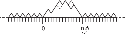
In this section we introduce and analyze a simple model of loop dynamics corresponding to $c=3/2$. Within the model, the loop is described by a fluctuating interface (or a string), interacting with an attractive substrate in $d=1+1$ dimensions. Here the interface height variable corresponds to the distance between complementary bases. The interface configurations are those of a restricted solid on solid (RSOS) model defined as follows (see Fig. (1)): Let $h_{i}=0,1,2\ldots$ be the height of the interface at site $i$. The heights satisfy $|h_{i}-h_{i+1}|=\pm 1$. Consider a loop between sites $0$ and $n$ (where $n$ is even) as shown in Fig. (1). Outside the loop the interface is bound to the substrate so that $h_{-2k}=h_{n+2k}=0$ and $h_{-2k-1}=h_{n+2k+1}=1$ for $k=0,1,\ldots$. Inside the loop the heights $h_{1}...h_{n-1}$ can take any non-negative value which is consistent with the RSOS conditions. For simplicity we allow only one end of the loop to fluctuate while the other is held fixed. This should not modify any of our results, since the dynamics of the two ends of long loops are uncorrelated with each other. We consider a random sequential dynamics in which the loop configuration and its length are free to fluctuate. Thus the dynamical moves are as follows:

as long as the resulting heights are non-negative and the RSOS condition is satisfied. For $i=n$ the loop length is changed according to the rules

where $n$ can decrease only if $h_{n-2}=0$. At the other end the height is fixed, $h_{0}=0$. It is straightforward to verify that the number of configurations of a loop of size $n$ is given by $2^{n}/n^{c}$ with $c=3/2$ for large $n$. This is a result of the fact that the number of walks of length $n$ in $d=1+1$ dimensions is $2^{n}$ and the probability of first return is $n^{-3/2}$. The ratio, $1/4$, between the two length changing processes in Eq. (12) is chosen such that in the large $n$ limit the loop is not biased to either grow or shrink. This corresponds to the model being at the denaturation transition point, which is determined by equating the free energies of the pinned segment and that of the open loop. Combining this with detailed balance yields the ratio between the rates. The parameter $\overline{\alpha}$ determines the rate of the length changing processes: $\overline{\alpha}=0$ corresponds to the dynamics of a loop of a fixed length. As $\overline{\alpha}$ is increased the length changing processes become faster. In the following subsection this model is generalized to include a power law potential between the interface and the substrate. This will allow us to study other values of $c$.

In a realization of this dynamics one of the $n+1$ attempts defined above, Eqs. (11) and (12), is chosen at any given time. Of these, $n-1$ are attempts to update the height at sites $1,2,\ldots,n-1$. The other two are attempts to update the position of the edge by a move either to the right or to the left. One attempted move of the edge defines a Monte Carlo sweep.

In order to test the validity of Eq. (2) we compare its predictions with results obtained from numerical simulations of the model above. In the numerical simulation we find good data collapse, when plotted against $t/n_{0}^{z}$ with $z\gtrsim 2$, depending on the value of $\overline{\alpha}$, rather than the expected Fokker-Planck value $z=2$. With these modified $z$ exponents the survival probability agrees well with the results obtained from the discrete version of the Fokker-Planck equation. The results are summarized in Fig. (2) where the survival probability is plotted as a function of the scaling variable $t/n_{0}^{2.2}$ and $t/n_{0}^{2.07}$ for $\overline{\alpha}=1$ and $\overline{\alpha}=0.1$ respectively, for several values of the loop size $n_{0}$. The question is whether the discrepancy in the value of $z$ is a result of a finite size effect or does it persist in the large $n_{0}$ limit. For the Fokker-Planck equation to properly describe the system it is essential to show that $z$ approaches $2$ in the large $n_{0}$ and $t$ limit.

In the following we argue that in fact the value $z=2.2$ in the case of $\overline{\alpha}=1$ (and $z=2.07$ for $\overline{\alpha}=0.1$) is a result of finite size effects. For large systems the value $z=2$ is expected to be recovered. To check this point we calculate numerically the variance of the loop size

where $\langle\cdot\rangle$ denotes an average over realizations of the dynamics. In order to evaluate the temporal growth of $w^{2}(t)$ we define a variable $\sigma_{+}(t)$ which takes the value $1$ if the length of the loop increases at time $t$ and $0$ otherwise. Similarly, we define $\sigma_{-}(t)$ and $\sigma_{0}(t)$ for steps which decrease the loop size and steps in which the loop size does not change, respectively. Clearly $\sigma_{+}(t)+\sigma_{-}(t)+\sigma_{0}(t)=1$. The dynamics of the chain, Eq. (12), implies that in the limit of large $n_{0}$ one has

where $\alpha=\overline{\alpha}/\max\{1,\overline{\alpha}\}$ in accordance with the random sequential dynamics. Denoting $U(t)\equiv\sigma_{+}(t)-\sigma_{-}(t)$, it is easy to see that

where

It is evident that a loop increasing step at time $t$, ($\sigma_{+}(t)=1$), is uncorrelated with steps which took place at time $\tau<t$. Thus $\langle\sigma_{+}(\tau)\sigma_{+}(t)\rangle=\langle\sigma_{-}(\tau)\sigma_{+}(t)\rangle=\alpha^{2}/64$. Numerically we find $\langle\sigma_{-}(\tau)\sigma_{-}(t)\rangle=\alpha^{2}/64$ (see Fig. (3)). Using these results we finally obtain

with $\langle\sigma_{+}(\tau)\sigma_{-}(t)\rangle_{c}\equiv\langle\sigma_{+}(\tau)\sigma_{-}(t)\rangle-\alpha^{2}/64$. Numerical simulations of the dynamics show strong correlation between $\sigma_{+}(\tau)$ and $\sigma_{-}(t)$ with an algebraic decay in $t-\tau$ (see Fig. (3)). It is interesting to note that the dynamics of the chain induces such long range temporal correlations between steps of the edge mediated by the loop dynamics.

By extrapolating the sum on the right hand side of Eq. (17) using the asymptotic form $B(t-\tau)^{-\gamma}$ with $B\approx 0.015$ and $\gamma\approx 1.2$, deduced from Fig. (3), we find that the sum converges to a non-zero value. This is demonstrated in Fig. (4) for $\overline{\alpha}=1$ and $\overline{\alpha}=0.1$. For example, in the case $\overline{\alpha}=1$ the sum converges to $\approx 0.84<\alpha=1$ indicating that $w^{2}(t)\approx 0.16t$ at large $t$, which in turn yields $z=2$. The slow power-law convergence towards the asymptotic value implies that it may require large systems to observe the long time behavior of Eq. (2.1).

In this section we generalize the model of the previous section to consider the case of arbitrary $c$. This can be done within a $d=1+1$ dimensional model by introducing a repulsive interaction between the substrate and the interface. Taking an interaction of the form $A/h^{2}$, where $h$ is the distance between the interface and the substrate and $A$ is a constant, results in an equilibrium weight of a loop of the form $1/n^{c}$. The exponent $c$ is related to the interaction strength $A$ [22, 23].

In order to derive the relation between $A$ and $c$ one notes that at the critical point the distribution of the distance between the interface and the substrate decays algebraically at large distances, $Q(h)\sim 1/h^{\kappa}$. It has been shown that for an interface model for which self-avoiding interactions play no role, the exponent $\kappa$ is related to the loop exponent $c$ by [24]

We proceed by introducing a specific model and evaluate $\kappa$ in terms of the interaction parameter $A$. One then obtains the loop exponent $c$ from Eq. (18). We consider an RSOS interface model with the Hamiltonian

where as before, $h_{i}=0,1,2...$, and $h_{i}-h_{i+1}=\pm 1$. In this Hamiltonian $\varepsilon>0$ represents the binding energy between the substrate and the interface. To evaluate $Q(h)$ we write down the eigenvalue equation of the transfer matrix corresponding to the Hamiltonian Eq. (19). For $h>1$ the equation is

Here $\lambda$ is the eigenvalue and $\Psi_{h}$ are the components of the eigenvector. The distance distribution is given by $Q(h)\propto\Psi_{h}^{2}$. At criticality the eigenvector component, at large $h$, has a form $\Psi(h)=1/h^{\kappa/2}$. By using this form in Eq. (20) we find the relation

Combining this with Eq. (18) yields

We now use the model, Eq. (19), to study numerically the dynamics of a loop with $c\neq 3/2$. The dynamics of the model is similar to that introduced in Sec. 2.2, but with the transition rates of Eq. (11) modified according to the Hamiltonian Eq. (19). Namely, the updating rates are given by

as long as the resulting heights are non-negative and the RSOS condition is satisfied. The presence of the long-range interactions also changes the ratio between the rates by which the loop grows ($R(n\to n+2)$) and shrinks ($R(n+2\to n)$). This ratio is given by

The critical temperature is found by equating the free energy of the loop with that of the bound segment. This yields

where $A-\varepsilon$ is the energy of a pair of sites in the bound segment and $4$ is the statistical weight of a pair of sites in the open loop. Combining this with Eq. (24) gives

We have simulated the dynamics of Eqs. (23) and (26) for $A=0.15$ and $A=0.5$. These values of $A$ correspond to $c\approx 1.74\;(<2)$ and $c\approx 2.12\;(>2)$ respectively. In Fig. (5) we present the loop size distribution for these two values of the parameter $A$. The resulting $c$ values fit well with the predictions.

In studying the survival probability of a loop we follow the same approach which was applied in the previous section for $c=3/2$. Similar results were obtained for the case of $c>3/2$. In Fig. (6) we present the survival probability as obtained from numerical simulations of the model. We find good data collapse, but again with a modified exponent $z=2.2$ for $\overline{\alpha}=1$. The scaling function fits well with that obtained from a numerical integration of a discrete version of Eq. (2).

We have also calculated the step-step autocorrelation function as for the case $c=3/2$ and found similar results. In particular, we find that the exponent $\gamma$ seems to have a weak dependence on $A$, with $\gamma\sim 1.4$ for both $A=0.15$ and $A=0.5$ (Figures not shown).

The DNA configurations can be represented by an alternating sequence of bound base-pairs and loops. We denote by $[k]$ a bound segment with length $k$ and $(l)$ a loop of length $l$, with $k,l>0$. A given configuration of the DNA is thus represented by $[k_{1}](l_{1})[k_{2}](l_{2})\ldots$. In terms of these variables the dynamics of the model is defined by the following rates:

• •

  Motion of a loop edge. This corresponds to the same processes which were considered in the dynamics of an isolated loop in the previous section.

  $$\begin{array}[]{lll}\;[k](l)\to[k-1](l+1)&&{\rm\;with\;rate}\;\;\;\left(\frac{l}{l+1}\right)^{c}\\ \;[k-1](l+1)\to[k](l)&&{\rm\;with\;rate}\;\;\;1\\ \;(l)[k]\to(l+1)[k-1]&&{\rm\;with\;rate}\;\;\;\left(\frac{l}{l+1}\right)^{c}\\ \;(l+1)[k-1]\to(l)[k]&&{\rm\;with\;rate}\;\;\;1\end{array}$$

These processes are executed as long as the lengths of the resulting loops and bound segments are non-zero.

• •

  Splitting and merging of loops

  $$\begin{array}[]{lll}\;(l_{1}+l_{2}+1)\to(l_{1})[1](l_{2})&&{\rm\;with\;rate}\;\;\;\frac{\sigma_{0}}{\zeta(c)}\left(\frac{l_{1}+l_{2}+1}{l_{1}l_{2}}\right)^{c}\\ \;(l_{1})[1](l_{2})\to(l_{1}+l_{2}+1)&&{\rm\;with\;rate}\;\;\;1\end{array}$$

  (27)

In addition we consider creation and annihilation of loops.

• •

  Creation and annihilation of loops

  $$\begin{array}[]{lll}\;[k_{1}+k_{2}+1]\to[k_{1}](1)[k_{2}]&&{\rm\;with\;rate}\;\;\;\frac{\sigma_{0}}{\zeta(c)(1-\sigma_{0})}\\ \;[k_{1}](1)[k_{2}]\to[k_{1}+k_{2}+1]&&{\rm\;with\;rate}\;\;\;1\end{array}$$

Here $\sigma_{0}$ is the cooperativity parameter, and $\zeta(c)=\sum_{n=1}^{\infty}n^{-c}$. It is straightforward to verify that the choice of rates satisfies detailed balance with respect to the equilibrium weight for the loop sizes at criticality $P(n)=\sigma_{0}\frac{n^{-c}}{\zeta(c)}$.

To check that indeed interactions between loops do not modify the asymptotic behavior of the autocorrelation function $C(t)$ we simulate the model Eq. (• ‣ 3.1)–(• ‣ 3.1). We use the experimental relevant value $\sigma_{0}=10^{-4}$ [19] and consider a DNA length of $100,000$ base-pairs. The autocorrelation is evaluated by monitoring the state of $1000$ base-pairs uniformly distributed within the DNA. Fig. (7) shows the results for various values of $c$ along with the theoretically expected slopes.

While the results for large values of $c$ agree well with the theory, there is a systematic deviation from the predicted slopes for smaller values of $c$ close to 2. These deviations could be attributed to the finite length of the simulated system. For example it is clear that for $c<2$ the autocorrelation function of a finite system decays to zero at long times rather than remaining constant. This is due to the fact that there is an upper cutoff on the loop size available. Only for an infinite system $C(t)$ is expected to remain constant ($=1$) at long times. In order to check this point we introduce an upper cutoff $N_{max}$ to the loop size in the equation for the autocorrelation function

The loop size $N_{max}$ is chosen so that it appears roughly one time during a run. For runs which are not too long this can be estimated using $\sigma_{0}LRP(N_{max})=1$, where L is the system size and R is the number of Monte-Carlo repetitions performed. In Fig. (8) the results of the simulations are compared with the theoretical expression, Eq. (28), which is summed numerically.

In summary, we find that our scaling predictions are generally confirmed by the numerical simulations of the many loops model. However, for values of $c$ close to $2$, deviations are found. These seems to be related to finite size effects.

References

- [1] For a review see R.M. Wartell, A.S. Benight, Phys. Rep. 126, 67 (1985); O. Gotoh, Adv. Biophys. 16, 1 (1983).
- [2] Y. Kafri, D. Mukamel and L. Peliti, Eur. Phys. J. B 27, 135 (2002).
- [3] M. Peyrard and A. R. Bishop, Phys. Rev. Lett. 62, 2755 (1989).
- [4] D. Poland, H.A. Scheraga, J. Chem. Phys. 45, 1456 (1966); J. Chem. Phys. 45, 1464 (1966).
- [5] M.E. Fisher, J. Chem. Phys. 45, 1469 (1966).
- [6] Y. Kafri, D. Mukamel, L. Peliti, Phys. Rev. Lett. 85, 4988 (2000).
- [7] U. Bockelmann, P. Thomen, B. Essevaz-Roulet, V. Viasnoff, F. Heslot, Biophys. J. 82, 1537 (2002).
- [8] B. EssevazRoulet, U. Bockelmann, F. Heslot, Proc. Natl. Acad. Sci. USA, 94, 11935 (1997).
- [9] C. Danilowicz, Y. Kafri, R.S. Conroy, V. W. Coljee, J. Weeks, M. Prentiss, Phys. Rev. Lett. 93, 078101 (2004).
- [10] C. Danilowicz, V. W. Coljee, C. Bouzigues, D. K. Lubensky, D. R. Nelson, M. Prentiss, Proc. Natl. Acad. Sci. USA, 100, 1694 (2003).
- [11] G. Altan-Bonnet, A. Libchaber, O. Krichevsky, Phys. Rev. Lett. 90, 138101 (2003).
- [12] T. Ambjornsson, S. K. Banik, O. Krichevsky, R. Metzler, Phys. Rev. Lett. 97, 128105 (2006).
- [13] T. Ambjornsson, S. K. Banik, O. Krichevsky O, R. Metzler R, Biophys. J. 92, 2674 (2007).
- [14] Y. Zeng, A. Montrichok, G. Zocchi, Phys. Rev. Lett. 91, 148101 (2003).
- [15] A. Hanke, R. Metzler, J. Phys. A: Math. Gen. 36, 473 (2003).
- [16] D.J. Bicout, E. Kats, Phys. Rev. E 70, 010902(R) (2004).
- [17] A. Bar, Y. Kafri and D. Mukamel, Phy. Rev. Lett. 98, 038103 (2007).
- [18] H. Kunz, R. Livi, A. Suto, J. Stat. Mech.: Theor. Exp., P06004 (2007).
- [19] R. Blossey, E. Carlon, Phys. Rev. E 68, 061911 (2003).
- [20] E.Carlon, E. Orlandini, A. L. Stella, Phys. Rev. Lett. 88, 198101 (2002).
- [21] M. S. Causo, B. Coluzzi and P. Grassberger,Phys. Rev. E 62, 3958 (2000).
- [22] R. K. P. Zia, R. Lipowsky, D. M. Kroll, Am. J. Phys. 56 160 (1988)
- [23] R. Lipowsky, Europhys. Lett. 15, 703 (1991).
- [24] M. Baiesi, E. Carlon, Y. Kafri, D. Mukamel, E. Orlandini, A. L. Stella, Phys. Rev. E.,67, (2003).
- [25] L. -H. Tang and H. Chaté, Phys. Rev. Lett. 86, 830 (2001).
- [26] G. Giacomin and F. L. Toninelli, Phys. Rev. Lett. 96, 070602 (2006).
- [27] S. Redner, A guide to first-passage processes, Cambridge University Press, Cambridge (UK) (2001)
- [28] D.K. Lubensky, D.R. Nelson, Phys. Rev. E 65, 031917 (2002)
- [29] P. Le Doussal, C. Monthus, D. S. Fisher, Phys. Rev. E. 59, 4795 (1999)
- [30] T. Garel, C. Monthus, Eur. Phys. J. B 46, 117 (2005)
- [31] M. Doi and S. F. Edwards, The Theory of Polymer Dynamics (Clarendon Press, Oxford, 1986).
- [32] R. Shusterman, S. Alon, T. Gavrinyov and O. Krichevsky, Phys. Rev. Lett. 92, 048303 (2004).
- [33] M. Abramowitz, and Stegun, I. A. (Eds.). Handbook of Mathematical Functions with Formulas, Graphs, and Mathematical Tables, 10th printing. New York: Dover (1972)