A Mathematical Theory of Stochastic Microlensing I.
Random Time-Delay Functions and Lensing Maps

A. O. Petters Email: petters@math.duke.edu Affiliation: Departments of Mathematics and Physics, Duke University, Science Drive, Durham, NC 27708, United States of America B. Rider Email: brider@euclid.colorado.edu Affiliation: Department of Mathematics, University of Colorado at Boulder, Campus Box 395 Boulder, CO 80309, United States of America A. M. Teguia Email: alberto@math.duke.edu Affiliation: Department of Mathematics, Duke University, Science Drive, Durham, NC 27708, United States of America

Abstract

Stochastic microlensing is a central tool in probing dark matter on galactic scales. From first principles, we initiate the development of a mathematical theory of stochastic microlensing. Beginning with the random time delay function and associated lensing map, we determine exact expressions for the mean and variance of these transformations. In addition, we derive the probability density function (p.d.f.) of a random point-mass potential, which form the constituent of a stochastic microlens potential. We characterize the exact p.d.f. of a normalized random time delay function at the origin, showing that it is a shifted gamma distribution, which also holds at leading order in the limit of a large number of point masses if the normalized time delay function was at a general point of the lens plane. For the large number of point masses limit, we also prove that the asymptotic p.d.f. of the random lensing map under a specified scaling converges to a bivariate normal distribution. We show analytically that the p.d.f. of the random scaled lensing map at leading order depends on the magnitude of the scaled bending angle due purely to point masses as well as demonstrate explicitly how this radial symmetry is broken at the next order. Interestingly, we found at leading order a formula linking the expectation and variance of the normalized random time delay function to the first Betti number of its domain. We also determine an asymptotic p.d.f. for the random bending angle vector and find an integral expression for the probability of a lens plane point being near a fixed point. Lastly, we show explicitly how the results are affected by location in the lens plane. The results of this paper are relevant to the theory of random fields and provide a platform for further generalizations as well as analytical limits for checking astrophysical studies of stochastic microlensing.

Keywords:

gravitational lensing, random mappings, probability, asymptotics

pacs

02.30.Nw, 98.62.Sb, 02.50.-r

I Introduction

Stochastic microlensing is the study of the deflection of light by a random collection of stars. In recent years, this subject has become a central tool in understanding the nature and distribution of dark matter on galactic scales (e.g., Schechter and Wambsganss [1]). This has raised the need for a rigorous framework for stochastic microlensing.

Research on stochastic microlensing has been mainly numerical, or at least semi-analytical, in flavor. Work in the early 1980’s included an analytical study of certain stochastic effects of microlensing by a single random lens (e.g., Vietri and Ostriker [2]). This was later extended to the case of multiple lenses using numerical simulations (e.g., Kayser, Refsdal, and Stabell [3]; Paczynski [4]). While successful in furthering our picture of stochastic microlensing, these simulations often cannot be checked analytically and are time-consuming. Some of the first analytical counterparts of the numerics were focused on the study of random surface brightnesses, bending angles, magnifications, and redshifts (e.g., Deguchi and Watson [5, 6]; Katz, Balbus, and Paczynski [7]; Schneider [8]; Turner, Ostriker, and Gott [9]; Vietri [10]). This was followed by numerical and semi-rigorous work characterizing the magnification probabilities and the expected number of microimages in a variety of lensing situations (e.g., Rauch et al. [11]; Wambsganss [12]; Wambsganss, Witt, and Schneider [13]). Recently, similar techniques were employed to study the distributions of microimages, magnifications, and time delay differences between images, with the last two applied directly to probe dark matter using flux-ratio anomalies (e.g., Granot, Schechter, and Wambsganss [14]; Keeton, and Moustakas [15]; Schechter, and Wambsganss [1]; Schechter, Wambsganss, and Lewis [16]; Tuntsov et al. [17]). In a more general context, Berry and collaborators also explored the statistical aspects of caustics in optical systems for the case of Gaussian random fields (see [18] and references therein).

This series aims to develop a mathematical theory of stochastic microlensing, starting from first principles. This fits in the general theory of random fields, namely, the study of random functions and their critical point structure (for more on random fields, see Adler and Taylor [19] and references therein). We derive new stochastic results, for a general point in the lens plane, about random time delay functions and lensing maps, which are transformations forming the core of microlensing theory. We determine the exact (as opposed to asymptotic) expectation and variance of both the lensing map and the point mass potential. Using the expected value of the components of the lensing map, we deduce, for a fixed image in the lens plane, the corresponding average position of the point it is mapped to in the light source plane. Furthermore, since point mass potentials form the density components of the time delay function, we use the exact formulas of their first and second moments to derive the asymptotic expectation and variance of the normalized time delay function in the large number of stars limit. We also reveal an interesting topological link, namely, at leading order we show that the expectation and variance of the normalized random microlensing time delay function is related to the first Betti number of the time delay functions’s domain.

Continuing our study of the normalized random time delay function, we establish that at the origin its exact p.d.f. is a shifted gamma distribution, and that this is asymptotically the case for an arbitrary point within the lens plane in the large number of stars limit. In the same limit, we prove that the p.d.f of a scaled lensing map converges to a bivariate Gaussian, with once again consistent asymptotic mean and variance. This analytical work shows that the p.d.f. of the random scaled lensing map at leading order term depends on the square of magnitude of the scaled bending angle due purely to point masses. It also illustrate how this radial symmetry is broken at the next order. Similarly, we note that the p.d.f. of the random time delay function at the origin depends only on the potential time delay due purely to point masses, a result also holding at leading order for an arbitrary point in the lens plane.

Taking our analysis further, we compute the probability that the image of a given point under the lensing map will be in a given disk in light the source plane, which provides information about the light source position. We deduce from these results the expectation, variance, and asymptotic p.d.f. of the bending angle vector at an arbitrary position in the lens plane. We also use these results to compute the probability that a point in the lens plane will be mapped in a certain neighborhood of “itself” in the light source plane. This study relates to the theory of fixed points, which was studied earlier by Petters and Wicklin [20] in the case of a deterministic lens system.

Overall, these first steps lay the foundation in terms of concepts, results, and tools for future analytical work on random time delay functions and lensing mappings, including lensing observables like magnification, arising from more complex stochastic mass distributions. The work can also help as a guide on tractable aspects of the general theory of random mappings.

We state the basic random microlensing framework in Section II. In Section III, we present the results of our study of the random time delay function, obtaining its expectation, variance, exact p.d.f. at the origin, and asymptotic p.d.f. at an arbitrary lens plane point. A similar presentation of results is done for the random lensing map in Section IV. In Section V, we apply our results about random lensing maps to random bending angle vectors and fixed points. The detailed proofs of these results are given in the Appendix.

Finally, the second paper in this program will explore the random shear and expected number of microimages produced by stochastic microlensing.

II Basic framework

Consider a microlensing situation where the light source is point-like and located at $y$ in ${\mathbb{R}}^{2}$ (the light source plane) and the gravitational lens is a collection of $g$ point masses (stars) that are randomly distributed over a region of the lens plane. This lensing scenario is modeled with the following gravitational lens potential, where all quantities are in dimensionless form (see [21, pp. 79, 104]):

\displaystyle\psi_{g}(x)=\frac{\kappa_{c}}{2}|x|^{2}-\frac{\gamma}{2}(x_{1}^{2}-x_{2}^{2})+\sum_{j=1}^{g}m_{j}\log|x-\xi_{j}|,

(1)

with $x=(x_{1},x_{2})$ in the lens plane $L=\{\xi_{1},\dots,\xi_{g}\}$ .

In a standard stochastic microlensing situation, the light source position $y$ is assumed to be a uniform random vector in ${\mathbb{R}}^{2}$ and the star positions $\xi_{j}=(U_{j},V_{j})$ are taken to be independent, identically distributed (i.i.d.) uniform random vectors in a region of the lens plane. The continuous matter density $\kappa_{c}$ , external shear $\gamma$ , masses $m_{j}$ , and number of stars $g$ are assumed fixed, unless stated to the contrary. The random lens potential (1) is widely used in studies of stochastic lensing due to stars (see [23, 21]).

Remark:

•

The constants $m_{j}$ are scalar multiples of the actual stars’ physical masses, but we shall continue to call them masses for simplicity (see [21, p. 102]).
•

A natural next step is to consider a lensing scenario where the masses are distributed isothermally in an elliptical galaxy. This is a work in progress.

Gravitational microlensing of a light source at position $y$ in ${\mathbb{R}}^{2}$ causes a change in a light ray’s arrival time that is captured analytically by the dimensionless random time delay function given as follows (see [21], p. 81):

T_{g,y}(x)=\frac{1}{2}|x-y|^{2}-\frac{\kappa_{c}}{2}|x|^{2}+\frac{\gamma}{2}(x_{1}^{2}-x_{2}^{2})-\sum_{j=1}^{g}m_{j}\log|x-\xi_{j}|.

(2)

Fermat’s Principle of stationary time states (see [21], p. 67): Light rays from the source at $y$ to the observer are characterized by critical points of the time delay function $T_{y}(x)$ , that is, the solutions $x$ in the lens plane $L$ , where $L={\mathbb{R}}^{2}-\{\xi_{1},\dots,\xi_{g}\}$ , of the equation

\displaystyle\nabla T_{y}(x)={\bf 0},

(3)

where the gradient $\nabla$ is with respect to the $x$ variable.

The corresponding dimensionless random lensing map $\eta_{g}:L\rightarrow{\mathbb{R}}^{2}$ , (the lens plane), is defined by (see [21], p. 81):

\eta_{g}(x)=x-\nabla\psi_{g}(x).

The advantage of the lensing map is that solutions $x$ of (3) are equivalent to solutions $x$ of the lens equation (see [21], p. 81):

\eta_{g}(x)=y,

which are preimages $x$ of $y$ under the lensing map $\eta_{g}$ . Solutions $x\in L$ of the lens equation are called lensed images.

Microlensing also causes light rays to bend. For a light ray passing through the point $x$ in the lens plane, the bending angle $\alpha_{g}(x)$ at $x$ is given by (see [21], p. 79):

\alpha_{g}(x)=\nabla\psi_{g}(x).

Assumptions and Notation

We shall abide by the following throughout the paper:

•

Rectangular coordinates $(u,v)$ are assumed in the lens plane $L$ .
•

All masses are equal, $m_{j}\equiv m\neq 0,$ for $j=1,\cdots,g$ .
•

The star positions $\xi_{i}=(U_{i},V_{i})$ are independent and uniformly distributed in the disk $B({\bf 0},R)$ of radius $R$ centered at ${\bf 0}$ , that is,

$(U_{i},V_{i})\sim{\rm Unif}\Bigl\{(u,v)\in L:|u|^{2}+|v|^{2}\leq R^{2}\Bigr\},\ \ \ \ \ i=1,\cdots,g.$
•

The quantities $R$ and $g$ are related by the following physical formula for the surface mass density $\kappa_{*}$ :

$\displaystyle\kappa_{*}$ $\displaystyle=$ $\displaystyle\frac{m~g}{R^{2}}.$ (4)

Unless otherwise stated assume that $\kappa_{*}$ is fixed.
•

Notation: For clarity, the statement

$\mbox{ ``}F(x)=G(x)+O(K(x))\quad\mbox{as}\ x\rightarrow\infty\mbox{''}$

means precisely that

$\lim_{x\rightarrow\infty}\frac{|F(x)-G(x)|}{K(x)}\leq C$

for some constant $C>0$ .
•

Notation: $\log^{\ell}A=(\log A)^{\ell}.$

III Results on The Random time delay function

We can write the time delay function as

T_{g,y}(x)=\frac{1}{2}|x-y|^{2}\ -\ \frac{\kappa_{c}}{2}|x|^{2}\ +\ \frac{\gamma}{2}(x_{1}^{2}-x_{2}^{2})\ +\ \sum_{j=1}^{g}W_{g,j}(x),

where

W_{g,j}(x)=-m\log|x-\xi_{j}|

is the point mass potential.

We define a “normalization” $T_{g,y}^{*}$ of $T_{g,y}$ as follows:

T_{g,y}^{*}(x)\equiv T_{g,y}(x)+g\,m\log R=\frac{1}{2}|x-y|^{2}-\frac{\kappa_{c}}{2}|x|^{2}+\frac{\gamma}{2}(x_{1}^{2}-x_{2}^{2})\ +\ \sum_{j=1}^{g}W_{g,j}^{*}(x),

where

W_{g,j}^{*}(x)=-m\log\frac{|x-\xi_{j}|}{R}

is the normalized point mass potential. Note that this normalization (of the time delay function) does not change the lensing map and relevant physical lensing quantities such as magnification, difference in arrival times between two images, etc.

III.1 Exact Moments and Probability Density Functions

The first and second moments of a random point mass potential are given by:

Proposition 1.

Let $x\in B({\bf 0},R)$ and $y\in{\mathbb{R}}^{2}$ (the light source plane). Then

E[W_{g,j}(x)]=\frac{\kappa_{*}(R-|x|)^{2}(1-2\log(R-|x|))}{2g}-\frac{2\kappa_{*}}{\pi g}\int_{R-|x|}^{R+|x|}rf(r,|x|)(\log r)dr,

and

\displaystyle E[W_{g,j}^{2}(x)]

\displaystyle=

\displaystyle\frac{m\kappa_{*}(R-|x|)^{2}\left[1+2(\log(R-|x|)-1)\log(R-|x|)\right]}{2g}+\frac{2m\kappa_{*}}{\pi g}\int_{R-|x|}^{R+|x|}rf(r,|x|)(\log^{2}r)dr,

where $f(r,|x|)={\rm Arccos}\Bigl(\frac{|x|^{2}+r^{2}-R^{2}}{2|x|r}\Bigr)$ for non-zero $x$ , and $f(r,0)=0$ .

Proof:

See Appendix. ∎

Both integrals in the above proposition are finite (and can be computed numerically). Hence, the expectation of $T_{g,y}(x)$ ,

E[T_{g,y}(x)]=\frac{1}{2}|x-y|^{2}-\frac{\kappa_{c}}{2}|x|^{2}+\frac{\gamma}{2}(x_{1}^{2}-x_{2}^{2})+gE[W_{g,j}(x)]

and its variance

{\rm Var}[T_{g,y}(x)]=gE[W_{g,j}^{2}(x)]-g(E[W_{g,j}(x)])^{2}

are also finite. Instead of pursuing exact expressions for the mean and the variance of $T_{g,y}^{*}(x)$ for general $x\in B\left({\bf 0},R\right)$ , we take an asymptotic approach:

Corollary 2.

Let $x\in B({\bf 0},R)$ and $y\in{\mathbb{R}}^{2}$ (the light source plane). In the large $g$ limit, we have

E[T_{g,y}^{*}(x)]=\frac{m}{2}\,g\ +\ O(g^{1/2}\log g)

and

{\rm Var}[T_{g,y}^{*}(x)]=\left(\frac{m}{2}\right)^{2}g\ +\ O(g^{1/2}\log^{2}g).

Proof:

See Appendix. ∎

Corollary 2 shows an interesting link that has a “stochastic Morse theoretic” flavor, namely, at leading order,

E[T_{g,y}^{*}(x)]=\frac{m}{2}B_{1}(D_{*}),\qquad{\rm Var}[T_{g,y}^{*}(x)]=\left(\frac{m}{2}\right)^{2}B_{1}(D_{*})

where $D_{*}=B\left({\bf 0},R\right)-\{\xi_{1},\cdots,\xi_{g}\}$ and $B_{1}(D_{*})$ is the first Betti number of $D_{*}$ . This is because $B_{1}(D_{*})=g$ , which is the number of “holes” in $D_{*}$ (e.g., [21, p. 399]).

We now derive the p.d.f.’s of the point mass potentials $W_{g,j}(x)$ and $W_{g,j}^{*}(x)$ :

Proposition 3.

For $x\in B({\bf 0},R)$ , the p.d.f. of $W_{g,j}(x)$ is given by:

\displaystyle f_{W_{g,j}(x)}(h)

\displaystyle=

\displaystyle\left\{\begin{array}[]{lr}\frac{2}{mR^{2}}\exp[-\frac{2h}{m}],&~~~~~-m\log(R-|x|)<h\\ A_{R,x}^{{}^{\prime}}(h),&~~~~-m\log(R+|x|)<h<-m\log(R-|x|)\\ 0,&~~~~h<-m\log(R+|x|),\end{array}\right.

where

$\displaystyle A_{R,x}(h)$	$\displaystyle=$	$\displaystyle 1-\Bigl(r_{h}\cos^{-1}\theta_{R,1}(h)+R^{2}\cos^{-1}\theta_{R,2}(h)-B_{R,x}(h)\Bigr)/(\pi R^{2}),$
$\displaystyle r_{h}$	$\displaystyle=$	$\displaystyle\exp[2h/m],$
$\displaystyle\theta_{R,1}(h)$	$\displaystyle=$	$\displaystyle(\|x\|^{2}+r_{h}^{2}-R^{2})/(2\|x\|r_{h}),$
$\displaystyle\theta_{R,2}(h)$	$\displaystyle=$	$\displaystyle(\|x\|^{2}+R^{2}-r_{h}^{2})/(2\|x\|R),$
$\displaystyle B_{R,x}(h)$	$\displaystyle=$	$\displaystyle\sqrt{(R+r_{h}-\|x\|)(d+r_{h}-R)(d+R-r_{h})(d+r_{h}+R)}/2.$

It then follows that the p.d.f. of $W_{g,j}^{*}(x)$ is:

\displaystyle f_{W_{g,j}^{*}(x)}(h)=\left\{\begin{array}[]{lr}\frac{2}{m}\exp[-\frac{2h}{m}],&~~~~~-m\log(1-\frac{|x|}{R})<h\\ A_{1,\frac{x}{R}}^{{}^{\prime}}(h),&~~~~-m\log(1+\frac{|x|}{R})<h<-m\log(1-\frac{|x|}{R})\\ 0,&~~~~h<-m\log(1+\frac{|x|}{R}).\end{array}\right.

Proof:

See Appendix. ∎

At the origin, we obtain the exact p.d.f. for the random time delay function:

Corollary 4.

The random variable $T_{g,y}^{*}({\bf 0})$ has a shifted gamma distribution with density

\displaystyle f_{T_{g,y}^{*}({\bf 0})}(h)

\displaystyle=

\displaystyle\left\{\begin{array}[]{lr}\Bigl(\frac{2}{m}\Bigr)^{g}\frac{(h-c)^{g-1}}{(g-1)!}\exp\left[-\frac{2(h-c)}{m}\right],&~~~~~h>c\\ ~~0,&~~~~~h<c,\end{array}\right.

where $c=|y|^{2}/2$ .

Proof:

From Proposition 3, we know that $W_{g,j}^{*}(0)$ is an exponential random variable with parameter $2/m$ . By independence, $\sum_{j=1}^{g}W_{g,j}^{*}(0)\sim\Gamma(g,2/m).$ ∎

A direct calculation using the result of Corollary 4 shows that the exact expectation and variance of the normalized random time delay function at the origin are given respectively as follows:

E[T_{g,y}^{*}({\bf 0})]=\frac{m}{2}\,g\ +\ c,\qquad{\rm Var}[T_{g,y}^{*}({\bf 0})]=\left(\frac{m}{2}\right)^{2}g,

which is consistent with Corollary 2.

Although Corollary 4 only gives the p.d.f. of $T_{g,y}^{*}({\bf 0})$ , it will play a central role in establishing the asymptotic p.d.f. of $T_{g,y}^{*}(x)$ for an arbitrary $x\in B({\bf 0},R)$ — see Theorem 5 below.

III.2 Asymptotic P.D.F. for the Time Delay Function

The expression of the p.d.f. $f_{T_{g,y}^{*}(x)}$ for arbitrary $x$ can be derived via convolution and equation (3), but is very cumbersome. As $g\rightarrow\infty$ though, the analysis simplifies.

Theorem 5.

For every $x\in B({\bf 0},R)$ , let $f_{T_{g,y}^{*}(x)}$ be the p.d.f. of $T_{g,y}^{*}(x)$ . In the large $g$ limit, we have:

	$\displaystyle f_{T_{g,y}^{*}(x)}(h)$	$\displaystyle=$	$\displaystyle f_{T_{g,y}^{*}({\bf 0})}(h-d_{1}(x,y))+O(g^{-3/2})$
		$\displaystyle=$	$\displaystyle\left\{\begin{array}[]{lr}\Bigl(\frac{2}{m}\Bigr)^{g}\frac{(h-d_{1}-c)^{g-1}}{(g-1)!}\exp\left[-\frac{2(h-d_{1}-c)}{m}\right],&~~~~~h>d_{1}+c\\ ~~0,&~~~~~h<d_{1}+c,\end{array}\right.\ \ \ \ \ \ O(g^{-3/2})$

where $d_{1}(x,y)=\frac{1}{2}|x-y|^{2}-\frac{\kappa_{c}}{2}|x|^{2}+\frac{\gamma}{2}(x_{1}^{2}-x_{2}^{2})$ .

Proof:

See Appendix. ∎

Theorem 5 shows that, at leading order, the p.d.f. $f_{T_{g,y}^{*}(x)}$ of the normalized time delay function $T_{g,y}^{*}(x)$ is a gamma distribution. Moreover, since

h-d_{1}(x,y)-c=\sum_{j=1}^{g}-m\log\left(\frac{|x-\xi_{j}|}{R}\right),

the p.d.f. $f_{T_{g,y}^{*}(x)}$ for any $x\in B({\bf 0},R)$ depends at leading order on the normalized potential time delay due purely to point masses.

IV Results on the Random lensing map

The lensing map $\eta_{g}:L\rightarrow{\mathbb{R}}^{2}$ is defined by

\eta_{g}(x)=x-\nabla\psi_{g}(x),

where $L={\mathbb{R}}^{2}-\{\xi_{1},\dots,\xi_{g}\}$ is the lens plane. The components of the lensing map are given by

\eta_{1,g}(x)=(1-\kappa_{c}+\gamma)x_{1}+\sum_{j=1}^{g}\frac{m(U_{j}-x_{1})}{R_{j}^{2}(x)},\qquad\eta_{2,g}(x)=(1-\kappa_{c}-\gamma)x_{2}+\sum_{j=1}^{g}\frac{m(V_{j}-x_{2})}{R_{j}^{2}(x)}

where $R_{j}^{2}(x)=(U_{j}-x_{1})^{2}+(V_{j}-x_{2})^{2}$ .

IV.1 Exact Expectation and Variance of the Lensing Map Components

The components $\eta_{1,g}(x)$ and $\eta_{2,g}(x)$ of the lensing map have the following basic statistics:

Proposition 6.

For $x=(x_{1},x_{2})\in L\cap B({\bf 0},R)$ , the exact expectations of the components of the lensing map are

E[\eta_{1,g}(x)]=\left[1-(\kappa_{c}+\kappa_{*})+\gamma\right]\,x_{1}~~~~~~~{\rm and}~~~~~~E[\eta_{2,g}(x)]=\left[1-(\kappa_{c}+\kappa_{*})-\gamma\right]\,x_{2}.

Both variables have infinite variance.

Proof:

See Appendix. ∎

Proposition 6 provides statistical information about the position values of the lensing map in the light source plane. In fact, suppose that an image position $x=(x_{1},x_{2})$ is given. The proposition gives:

E[\eta_{1,g}(x_{1})]=  \left[1-(\kappa_{c}+\kappa_{*})+\gamma\right]\,x_{1},\qquad E[\eta_{1,g}(x_{2})]=\left[1-(\kappa_{c}+\kappa_{*})-\gamma\right]\,x_{2}.

If $x={\bf 0}$ , then on average the values of $\eta_{g}({\bf 0})$ are isotropically distributed around the origin in the light source plane. More generally, we obtain the following:

•

Case I (“macro-minimum”): $1-(\kappa_{c}+\kappa_{*})+\gamma>0$ and $1-(\kappa_{c}+\kappa_{*})-\gamma>0$ . If $x$ lies in a given quadrant of the lens plane, then on average the random lensing map will send $x$ over to the same quadrant in the light source plane.
•

Case II (“macro-saddle”): $1-(\kappa_{c}+\kappa_{*})+\gamma>0$ and $1-(\kappa_{c}+\kappa_{*})-\gamma<0$ . If $x$ lies in quadrant I of the lens plane, then on average the random lensing map will send $x$ over to quadrant IV in the light source plane. Similarly, we obtain results for the other quadrants.
•

Case III (“macro-maximum”): $1-(\kappa_{c}+\kappa_{*})+\gamma<0$ and $1-(\kappa_{c}+\kappa_{*})-\gamma<0$ . If $x$ lies in given quadrant of the lens plane, then on average the random lensing map will send $x$ over in the light source plane to the quadrant symmetric with respect to the origin (e..g, quadrant I goes to III on average).

IV.2 Asymptotic P.D.F. of the Lensing Map

For the remainder of the paper, we shall assume that

R^{2}=g/\pi,\qquad g>1,

which gives $\kappa_{*}=\pi m$ and ignores the known case with $g=1$ (single star lens). Also, we suppose that the random lensing map has an absolutely continuous cumulative distribution function. Then:

Theorem 7.

Let $x=(x_{1},x_{2})\in L\cap B\left({\bf 0},R\right)$ be fixed. The p.d.f. of the scaled lensing map $\frac{\eta_{g}(x)}{\sqrt{\log g}}$ is given in the large $g$ limit by:

	$\displaystyle f_{\frac{\eta_{g}(x)}{\sqrt{\log g}}}(\tilde{h},\tilde{k})$	$\displaystyle=$	$\displaystyle\frac{e^{-\frac{(\tilde{h}-\tilde{a}_{1})^{2}+(\tilde{k}-\tilde{a}_{2})^{2}}{2\tilde{\sigma}_{g}^{2}}}}{(\sqrt{2\pi}\tilde{\sigma}_{g})^{2}}\left[1\ -\ \frac{\kappa_{*}}{\sqrt{\log g}}\ \frac{x_{1}(\tilde{h}-\tilde{a}_{1})+x_{2}(\tilde{k}-\tilde{a}_{2})}{\tilde{\sigma}_{g}^{2}}\right.~~~~~~~~~~~~~~~$		(19)
			$\displaystyle\left.~~~~~~~~~~~~~~~+\frac{\kappa_{*}^{2}}{4\pi}\ \frac{((\tilde{h}-\tilde{a}_{1})^{2}+(\tilde{k}-\tilde{a}_{2})^{2})-2\tilde{\sigma}_{g}^{2}}{\tilde{\sigma}_{g}^{4}}\ \frac{\log(\log g)}{\log g}\right]+O\Bigl(\frac{1}{\log g}\Bigr),$		(19)

where $(\tilde{h},\tilde{k})$ are the possible values of $\frac{\eta_{g}(x)}{\sqrt{\log g}}$ and

	$\displaystyle\tilde{a}_{1}=\frac{(1-\kappa_{c}+\gamma)x_{1}}{\sqrt{\log g}},$		$\displaystyle\qquad\tilde{a}_{2}=\frac{(1-\kappa_{c}-\gamma)x_{2}}{\sqrt{\log g}},$
	$\displaystyle\tilde{\sigma}_{g}=\frac{\sigma_{g}}{\sqrt{\log g}},$		$\displaystyle\qquad\sigma_{g}=\frac{\kappa_{}}{\sqrt{\pi}}\,\sqrt{\log(B\,g^{1/2})},\qquad B=\frac{2\sqrt{\pi}e^{1-\gamma_{e}}}{\kappa_{}}\,(\gamma_{e}\ \mbox{is the Euler constant}).$

The p.d.f.s of the components of the scaled lensing map are:

f_{\frac{\eta_{i,g}(x)}{\sqrt{\log g}}}(\tilde{c})=\frac{e^{-\frac{(\tilde{c}-\tilde{a}_{i})^{2}}{2\tilde{\sigma}_{g}^{2}}}}{\sqrt{2\pi}\,\tilde{\sigma}_{g}}\Bigl[1-\frac{\kappa_{*}}{\sqrt{\log g}}\frac{x_{i}(\tilde{c}-\tilde{a}_{i})}{\tilde{\sigma}_{g}^{2}}+\frac{\kappa_{*}^{2}}{4\pi}\frac{(\tilde{c}-\tilde{a}_{i})^{2}-\tilde{\sigma}_{g}^{2}}{\tilde{\sigma}_{g}^{4}}\,\frac{\log(\log g)}{\log g}\Bigr]+O\Bigl(\frac{1}{\log g}\Bigr)

for $i=1,2.$ For notational simplicity, we use $\tilde{c}$ to represent the possible values of both $\eta_{1,g}(x)$ and $\eta_{2,g}(x)$ .

Proof:

See Appendix. ∎

Observe that the p.d.f. of the scaled lensing map $f_{\frac{\eta_{g}(x)}{\sqrt{\log g}}}$ depends on $x$ in its leading order term. Furthermore, the fact that

{\rm Var}\left[\frac{\eta_{i,g}(x)}{\sqrt{\log g}}\right]=\infty,\qquad i=1,2,

makes applying a standard Central Limit Theorem unwieldy, thus the method of proof presented in the Appendix.

Theorem 7 shows that at leading order, the p.d.f. of the scaled lensing map is bivariate normal and illustrates how at the next order the p.d.f. deviates from normality. Moreover, since

(\tilde{h}-{\tilde{a}}_{1},\tilde{k}-{\tilde{a}}_{2})=\frac{\alpha_{g}(x)}{\sqrt{\log g}}\equiv\tilde{\alpha}_{g}^{*},

which is the scaled bending angle due purely to stars, the quantity $(\tilde{h}-{\tilde{a}}_{1})^{2}+(\tilde{k}-{\tilde{a}}_{2})^{2}$ in (19) is $|\tilde{\alpha}_{g}^{*}|^{2}$ . In other words, the leading factor of the p.d.f. of the scaled lensing map depends on the square of the magnification of the scale bending angle due to stars. This radial symmetry is broken at the next order term since there is a dependence on the individual components of the scaled bending angle.

We now discuss several consequences of Theorem 7.

Corollary 8.

As $g\rightarrow\infty$ with fixed $x\in{\mathbb{R}}^{2}$ , we have:

\Bigl(\frac{\eta_{1,g}(x)}{\sqrt{\log g}},\frac{\eta_{2,g}(x)}{\sqrt{\log g}}\Bigr)\Rightarrow(\eta_{1,\infty},\eta_{2,\infty}).

Here “ $\Rightarrow$ ” denotes distributional convergence and $(\eta_{1,\infty},\eta_{2,\infty})$ is a bivariant normal random vector with independent mean-zero normal random variables as components, each with variance $\kappa_{*}^{2}/(2\pi)$ .

Proof:

See Appendix. ∎

We can readily obtain the p.d.f. of the unscaled lensing map:

Corollary 9.

Let $x=(x_{1},x_{2})\in L$ be fixed. The p.d.f. of $\eta_{g}(x)$ is given in the large $g$ limit by:

	$\displaystyle f_{\eta_{g}(x)}(h,k)$	$\displaystyle=$	$\displaystyle\frac{e^{-\frac{(h-a_{1})^{2}+(k-a_{2})^{2}}{2\sigma_{g}^{2}}}}{\Bigl(\sqrt{2\pi}\sigma_{g}\Bigr)^{2}}\Bigl[1-\kappa_{*}\frac{x_{1}(h-a_{1})+x_{2}(k-a_{2})}{\sigma_{g}^{2}}$		(20)
			$\displaystyle~~~~~~~~+\frac{\kappa_{*}^{2}}{4\pi}\ \frac{\Bigl((h-a_{1})^{2}+(k-a_{2})^{2}-2\sigma_{g}^{2}\Bigr)}{\sigma_{g}^{4}}H(g)\Bigr]+O\Bigl(\frac{1}{\log^{2}g}\Bigr),$		(20)

with the possible values of the random vector $\eta_{g}(x)$ written as $(h,k)$ . Here $\sigma_{g}$ and $H(g)$ are as defined in Theorem 7, and

a_{1}=(1-\kappa_{c}+\gamma)x_{1},\qquad a_{2}=(1-\kappa_{c}-\gamma)x_{2},\qquad H(g)=\log(\log g).

Proof:

First, note that the possible values of $\eta_{g}(x)$ and $\frac{\eta_{g}(x)}{\sqrt{\log g}}$ are related by

\displaystyle\tilde{h}=\frac{h}{\sqrt{\log g}},

\displaystyle\qquad\tilde{k}=\frac{k}{\sqrt{\log g}}.

We know that

f_{\eta_{g}(x)}(h,k)~=~\frac{1}{\log g}f_{\frac{\eta_{g}(x)}{\sqrt{\log g}}}(\tilde{h},\tilde{k})~=~\frac{1}{\log g}f_{\frac{\eta_{g}(x)}{\sqrt{\log g}}}\left(\frac{h}{\sqrt{\log g}},\frac{k}{\sqrt{\log g}}\right).

The result then follows directly from equation (19). ∎

Let us consider the leading function in equation (20), namely,

{\cal F}_{g,x}(h,k)=\frac{e^{-\frac{(h-a_{1})^{2}+(k-a_{2})^{2}}{2\sigma_{g}^{2}}}}{\Bigl(\sqrt{2\pi}\sigma_{g}\Bigr)^{2}}\left[1-\kappa_{*}\frac{x_{1}(h-a_{1})+x_{2}(k-a_{2})}{\sigma_{g}^{2}}\ +\ \frac{\kappa_{*}^{2}}{4\pi}\ \frac{\Bigl((h-a_{1})^{2}+(k-a_{2})^{2}-2\sigma_{g}^{2}\Bigr)}{\sigma_{g}^{4}}H(g)\right],

where $x\in B({\bf 0},R)$ and $(h,k)\in{\mathbb{R}}^{2}$ . Note that $H(g)>0$ if $g\geq 3$ . The function ${\cal F}_{g,x}$ is actually a p.d.f. for $|x|$ sufficiently small and $g\geq 3$ . In fact, under the latter, we have ${\cal F}_{g,x}(h,k)\geq 0~$ for all $(h,k)\in{\mathbb{R}}^{2}$ . Moreover, integration-by-parts gives:

\int_{{\mathbb{R}}^{2}}{\cal F}_{g,x}(h,k)\,dhdk=1.

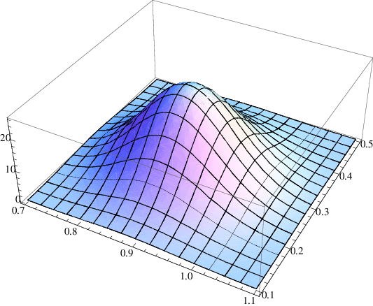
Hence, the function ${\cal F}_{g,x}$ is a p.d.f. on ${\mathbb{R}}^{2}$ for $|x|$ sufficiently small and $g\geq 3$ . Figure 1 depicts the graph of ${\cal F}_{g,x}$ with $x=(x_{1},x_{2})=(0.2,0)$ , $\kappa_{c}=0.405,~\gamma=0.3,~\kappa_{*}=0.045,$ and $g=10^{6}$ .

Refer to caption — Figure 1: Asymptotic p.d.f. of the random lensing map in the large number of stars limit.

Furthermore, there is enough control in the p.d.f. $f_{\eta_{g}(x)}$ to perform the expectation integrals to obtain:

Corollary 10.

Let $x\in L$ the lens plane. In limit $g\rightarrow\infty$ , the expectations of the components $\eta_{1,g}(x),\eta_{2,g}(x)$ of the lensing map are given by

E[\eta_{i,g}(x)]\simeq\left[1-(\kappa_{c}+\kappa_{*})+(-1)^{i+1}\gamma\right]\,x_{i},~~~~i=1,2.

Also, the variances of the lensing map components are infinite:

{\rm Var}[\eta_{i,g}(x)]\simeq\frac{\kappa_{*}^{2}}{\pi}[\log(B\,g^{1/2})+\frac{1}{2}\log\log g-\pi x_{i}^{2}]=\sigma_{g}^{2}\ +\ \frac{\kappa_{*}^{2}}{2\pi}\log\log g\ -\ \kappa_{*}^{2}\,x_{i}^{2},\ \ g\rightarrow\infty,~~~~~i=1,2.

Proof:

This result is obtained from Corollary 9 (see equation (20)) by computing the expected value and the variance of the random vector with density ${\cal F}_{g,x}(h,k)$ . ∎

Corollary 10 shows that the expectation from the asymptotic p.d.f. ${\cal F}_{g,x}$ is consistent with the findings in Proposition 6. We also have consistency for the variance as $g\,\rightarrow\,\infty$ . Note that in the leading order of Corollary 10 the divergent variance depends on the position $x$ .

Next, observe that given $g>1$ , the normal leading factor of the p.d.f. $f_{\eta_{g}(x)}$ is maximized at

{\bf a}=(a_{1},a_{2})=((1-\kappa_{c}+\gamma)x_{1},(1-\kappa_{c}-\gamma)x_{2}).

The following explores the probability that $\eta_{g}(x)$ is located in a neighborhood of the maximum:

Corollary 11.

Let $x=(x_{1},x_{2})\in L$ , fix $r_{0}\in{\mathbb{R}}$ , and let $n$ be a positive integer. The probability that the distance between $\eta_{g}(x)$ and the point ${\bf a}=(a_{1},a_{2})$ is between $(n-1)r_{0}$ and $nr_{0}$ , is given in the large $g$ limit by

	$\displaystyle P\Bigl[(n-1)r_{0}\leq\left\|\eta_{g}(x)-{\bf a}\right\|\leq nr_{0}\Bigr]$	$\displaystyle=$	$\displaystyle\frac{\exp[-\frac{(n^{2}+1)r_{0}^{2}}{2\sigma_{g}^{2}}]}{4\pi\sigma_{g}^{4}}\Bigl[e^{\frac{nr_{0}^{2}}{\sigma_{g}^{2}}}(4\pi\sigma_{g}^{4}+(n-1)^{2}r_{0}^{2}\kappa_{*}^{2}\log\log g)$		(21)
			$\displaystyle~~~~~~~~~~~~~~~~~~~~~~~~~-e^{\frac{r_{0}^{2}}{2\sigma_{g}^{2}}}(4\pi\sigma_{g}^{4}+n^{2}r_{0}^{2}\kappa_{*}^{2}\log\log g)\Bigr]+O\left(\frac{1}{\log^{2}g}\right).$		(21)

Proof:

See Appendix. ∎

Notice that the displayed leading terms in equation (21) are independent of the position $x$ , continuous matter density $\kappa_{c}$ , and external shear $\gamma$ .

Corollary 11, combined with the lens equation, provides probabilistic information about the angular position of the light source. Indeed, for $n=1$ the corollary gives the probability of $\eta_{g}(x)$ lying in a disk of angular radius $r_{0}$ centered at ${\bf a}$ , while for $n\geq 1$ we obtain the probability of $\eta_{g}(x)$ lying in an annular region between radii $(n-1)r_{0}$ and $nr_{0}$ centered at ${\bf a}$ . For illustration, we compute these probabilities in some specific cases:

p_{0.1}(n)=P\Bigl[(n-1)/10\leq\left|\eta_{g}(x)-{\bf a}\right|\leq n/10\Bigr]

and

\tilde{p}_{0.1}(n)=P\Bigl[0\leq|\eta_{g}(x)-{\bf a}|\leq n/10\Bigr]=\sum_{\ell=1}^{n}p_{0.1}(\ell),

for $n=1,2,3$ with the constants $r_{0}=0.1$ , $\kappa_{*}=0.045$ , and $g=10^{6}$ . The probabilities are given in Table I.

$n$	$1$	2	3
$p_{0.1}(n)$	$0.5595$	$0.4063$	$0.0337$
$\tilde{p}_{0.1}(n)$	$0.5595$	$0.9658$	$0.9995$

Table I: Probabilities of a lensing map’s value lying in various annuli (second row) and disks (third row).

The second row of Table I shows that the lensing map value $\eta_{g}(x)$ has a $56\%$ probability of lying inside the disk of angular radius $r_{0}=0.1$ centered at ${\bf a}$ , but a $97\%$ probability of lying within radius $2r_{0}$ . The probability of being in the outermost annulus $2\,r_{0}\leq\left|\eta_{g}(x)-{\bf a}\right|\leq 3\,r_{0}$ drops dramatically to $3\%$ .

V Results of the Random bending angle and fixed points

We now use our study of the lensing map to obtain probabilistic information about the bending angle vector and lensing fixed points.

V.1 Asymptotic P.D.F. of the Bending Angle

Recall that the bending angle vector $\alpha_{g}(x)$ is given by $\alpha_{g}(x)=\nabla\psi_{g}(x).$ Its asymptotic behavior is given below:

Corollary 12.

Let $x=(x_{1},x_{2})\in L$ . The p.d.f. of the bending angle vector is given in the large $g$ limit by

	$\displaystyle f_{\alpha_{g}(x)}(h^{},k^{})$	$\displaystyle=$	$\displaystyle\frac{e^{-\frac{(h^{}-a_{1}^{})^{2}+(k^{}-a_{2}^{})^{2}}{2\sigma_{g}^{2}}}}{\Bigl(\sqrt{2\pi}\sigma_{g}\Bigr)^{2}}\Bigr[1-\kappa_{}\frac{x_{1}(h^{}-a_{1}^{})+x_{2}(k^{}-a_{2}^{*})}{\sigma_{g}^{2}}$		(22)
			$\displaystyle\hskip 93.95122pt+\ \frac{\kappa_{}^{2}}{4\pi}\ \frac{\Bigl((h^{}-a_{1}^{})^{2}+(k^{}-a_{2}^{*})^{2}-2\sigma_{g}^{2}\Bigr)}{\sigma_{g}^{4}}\,\log(\log g)\Bigr]+O\Bigl(\frac{1}{\log^{2}g}\Bigr),$		(22)

where $(h^{*},k^{*})$ denotes the possible values of the random vector $\alpha_{g}(x)$ and $(a_{1}^{*},a_{2}^{*})=((\kappa_{c}-\gamma)x_{1},(\kappa_{c}+\gamma)x_{2}$ , while $\sigma_{g}$ is defined in Theorem 7. In other words, for sufficiently large $g$ , the bending angle is approximately a bivariate normal whose components $\alpha_{1,g}(x)$ and $\alpha_{2,g}(x)$ are normal random variables with respective means

\left[-(\kappa_{c}+\kappa_{*})+\gamma\right]\,x_{1}~~~{\rm and}~~~\left[-(\kappa_{c}+\kappa_{*})-\gamma\right]\,x_{2},

and variances diverging at leading order as

\frac{\kappa_{*}^{2}}{\pi}[\log(B\,g^{1/2})+\frac{1}{2}\log\log g-\pi x_{1}^{2}]~~~{\rm and}~~~\frac{\kappa_{*}^{2}}{\pi}[\log(B\,g^{1/2})+\frac{1}{2}\log\log g-\pi x_{2}^{2}],

respectively.

Proof:

By definition, we have $\alpha_{g}(x)=x-\eta_{g}(x)=\tilde{x}+{\mathbb{N}}_{g}(x)$ , where $\tilde{x}=((-\kappa_{c}+\gamma)x_{1},(-\kappa_{c}-\gamma)x_{2})$ . The corollary then follows from properties of independent random variables, Theorem 7, and some of its corollaries. ∎

When $x={\bf 0}$ , the second part of Corollary 12 recovers, in leading order, earlier results by Katz, Balbus, and Paczynski [7] and Schneider, Ehlers, and Falco (see [23], p. 325). Also note that from the discussion after Theorem 7, we have that the leading order term depends only on the squared magnitude of the bending angle due purely to point masses, and the next term breaks this radial symmetry.

V.2 Fixed Points

Lensed images of a light source usually do not appear at the same angular position of the light source. In the case where they do, they are called fixed points, which is a notion introduced in gravitational lensing by Petters and Wicklin [20]. More precisely, fixed points of the lensing map $\eta_{g}$ are points $x\in L$ such that

\eta_{g}(x)=x

or equivalently, points where the bending angle vector vanishes. $\alpha_{g}(x)={\bf 0}.$ Since $\alpha_{g}$ is a continuous random vector, we have $P[\alpha_{g}(x)={\bf 0}]=0.$ Nevertheless, we can study how close $\eta_{g}(x)$ is to $x$ .

Corollary 13.

Let $x\in B({\bf 0},R)\subset L$ and $\epsilon>0$ . The probability that $\eta_{g}(x)$ is within $\epsilon$ from $x$ in the light source plane is given by

P\left[\left|\eta_{g}(x)-x\right|\leq\epsilon\right]=\int_{B({\bf 0},\epsilon)}\,f_{\alpha_{g}(x)}(h^{*},k^{*})\,dh^{*}dk^{*}.

Proof:

This follows directly from Corollary 12 and the above discussion. ∎

VI Conclusion

We presented first steps in the development of a mathematical theory of stochastic microlensing that focused on the building blocks of the theory, namely, the random time delay function and random lensing map. We derived exact analytical formulas for the expectation and variance of the random time delay function and random lensing map about any point. In the large limit of stars, we found a simple asymptotic expression for the expectation and variance of a normalized time delay function at an arbitrary point. For the same limit, we highlighted an interesting link between the leading order term of the expectation and variance of our normalized random time delay function and the first Betti number of its domain. In addition, the asymptotic p.d.f.s of both the normalized time delay function and the scaled lensing map were characterized in the large number of stars limit: The asymptotic p.d.f. of the former is a shifted gamma density at leading order, while for the latter the p.d.f. is a bivariate Gaussian distribution. The p.d.f. of the random scaled lensing map is also shown to depend on the magnitude of the scaled bending angle due purely to point masses at leading order and we illustrated explicitly how this radial symmetry fails at the next order. We also derived the asymptotic p.d.f. of the random bending angle vector and gave an estimate of the probability of a lens plane point being close to a fixed point. Overall, the paper determined and illustrated new analytical results about the microlensing behavior of random time delay functions and random lensing maps about an arbitrary point of the lens plane.

In Paper II of this series, we shall explore the microlensing random shear and expected number of microimages.

VII Acknowledgments

AMT would like to thank Robert Adler, Jonathan Mattingly, and Andrea Watkins for useful discussions. AOP acknowledges the support of NSF Grants DMS-0707003 and AST-0434277-02.

Appendix A Proofs—The Random Time Delay Function

Proposition 1. Let $x\in B({\bf 0},R)$ and $y\in{\mathbb{R}}^{2}$ (the light source plane). Then

E[W_{g,j}(x)]=-\frac{\kappa_{*}(R-|x|)^{2}(-1+2\log(R-|x|))}{2g}-\frac{2\kappa_{*}}{\pi g}\int_{R-|x|}^{R+|x|}rf(r,|x|)(\log r)dr,

and

	$\displaystyle E[W_{g,j}^{2}(x)]$	$\displaystyle=$	$\displaystyle\frac{m\kappa_{*}(R-\|x\|)^{2}\left[1+2(\log(R-\|x\|)-1)\log(R-\|x\|)\right]}{2g}$
			$\displaystyle~~~~~~~~~~~~~~~~~~~~~~~+\frac{2m\kappa_{*}}{\pi g}\int_{R-\|x\|}^{R+\|x\|}rf(r,\|x\|)(\log^{2}r)dr,$

where $f(r,|x|)={\rm Arccos}\Bigl(\frac{|x|^{2}+r^{2}-R^{2}}{2|x|r}\Bigr)$ for non-zero $x$ , and $f(r,0)=0$ .

Proof of Proposition 1:

Let $x=(x_{1},x_{2})\in B({\bf 0},R)\cap L$ and $y\in{\mathbb{R}}^{2}$ . Translate the rectangular coordinates $(u,v)$ so that its origin ${\bf 0}$ moves to position $x$ . Denote the resulting new coordinates by $(u^{\prime},v^{\prime})$ and its origin by ${\bf 0}^{{}^{\prime}}$ . In the system $(u^{\prime},v^{\prime})$ , the old origin ${\bf 0}$ now has coordinates $(u^{\prime},v^{\prime})=-x$ . Define $\omega_{0}$ to be the unique principal angle with $\cos\omega_{0}=x_{1}/|x|$ , $\sin\omega_{0}=x_{2}/|x|$ , and let $\omega\equiv\omega_{0}+\pi$ . Rotate the rectangular coordinates $(u^{\prime},v^{\prime})$ counterclockwise by angle $\omega$ to obtain new coordinates $(u^{\prime\prime},v^{\prime\prime})$ with origin ${\bf 0}^{\prime\prime}={\bf 0}^{\prime}$ . Note that the old origin $\bf 0$ now lies at position $(u^{\prime\prime},v^{\prime\prime})=(|x|,0)\equiv x^{\prime\prime}$ on the positive $u^{\prime\prime}$ -axis. Finally, let $(\theta,r)$ denote polar coordinates in the frame $(u^{\prime\prime},v^{\prime\prime})$ . The figure below illustrate some of these change of variables.

We have

E[W_{g,j}(x)]=-mE[\log|x-\xi_{j}|]

and

$\displaystyle E[\log\|x-\xi_{j}\|]$	$\displaystyle=$	$\displaystyle\frac{1}{2\pi R^{2}}\int_{B({\bf 0},R)}\log[(u-x_{1})^{2}+(v-x_{2})^{2}]dudv$
	$\displaystyle=$	$\displaystyle\frac{1}{2\pi R^{2}}\Bigl[\int_{B({\bf 0}^{{}^{\prime}},R-\|x\|)}\,\log\left[(u^{\prime})^{2}+(v^{\prime})^{2}\right]\,du^{\prime}dv^{\prime}$
		$\displaystyle~~~~~~~~~+\int_{B(-x,R)\backslash B({\bf 0}^{{}^{\prime}},R-\|x\|)}\,\log\left[(u^{\prime})^{2}+(v^{\prime})^{2}\right]\,du^{\prime}dv^{\prime}\Bigr].$

For $x={\bf 0}$ , the result follows. Suppose $x\neq{\bf 0}$ . Then

$\displaystyle E[\log\|x-\xi_{j}\|]$	$\displaystyle=$	$\displaystyle\frac{1}{2\pi R^{2}}\Bigl[\int_{B({\bf 0}^{\prime\prime},R-\|x\|)}\,\log\left[(u^{\prime\prime})^{2}+(v^{\prime\prime})^{2}\right]\,du^{\prime\prime}dv^{\prime\prime}$
		$\displaystyle~~~~~~~~~+\int_{B(x^{\prime\prime},R)\backslash B({\bf 0}^{\prime\prime},R-\|x\|)}\,\log\left[(u^{\prime\prime})^{2}+(v^{\prime\prime})^{2}\right]\,du^{\prime\prime}dv^{\prime\prime}\Bigr]$
	$\displaystyle=$	$\displaystyle\frac{1}{\pi R^{2}}\int_{0}^{R-\|x\|}r(\log r)\Bigl(\int_{0}^{2\pi}d\theta\Bigr)dr+\frac{1}{\pi R^{2}}\int_{R-\|x\|}^{R+\|x\|}r(\log r)\Bigl(\int_{-f(r,\|x\|)}^{f(r,\|x\|)}d\theta\Bigr)dr$
	$\displaystyle=$	$\displaystyle\frac{2}{R^{2}}\int_{0}^{R-\|x\|}r\log rdr+\frac{2}{\pi R^{2}}\int_{R-\|x\|}^{R+\|x\|}rf(r,\|x\|)\log rdr$
	$\displaystyle=$	$\displaystyle\frac{(R-\|x\|)^{2}(-1+2\log(R-\|x\|))}{2R^{2}}+\frac{2}{\pi R^{2}}\int_{R-\|x\|}^{R+\|x\|}rf(r,\|x\|)(\log r)dr,$

which gives the mean. The second moment is obtained similarly. ∎

Corollary 2. Let $x\in B({\bf 0},R)$ and $y\in{\mathbb{R}}^{2}$ (the light source plane). In the large $g$ limit, we have

E[T_{g,y}^{*}(x)]=\frac{m}{2}g+O(g^{1/2}\log g)

and

{\rm Var}[T_{g,y}^{*}(x)]=\frac{m^{2}}{4}g+O(g^{1/2}\log^{2}g).

Proof of Corollary 2:

Let $d_{n}(x,y)=\Bigl(\frac{1}{2}|x-y|^{2}-\frac{\kappa_{c}}{2}|x|^{2}+\frac{\gamma}{2}(x_{1}^{2}-x_{2}^{2})\Bigr)/n,\ \ n\in\mathbb{N}$ for arbitrary $x$ .

$\displaystyle E[T_{g,y}^{*}(x)]$	$\displaystyle=$	$\displaystyle d_{1}(x,y)+gE[W_{g,y}(x)]+mg\log R$
	$\displaystyle=$	$\displaystyle\frac{\kappa_{}R^{2}}{2}\Bigl[\frac{2}{\kappa_{}R^{2}}d_{1}(x,y)\ +\ (1-\|x\|/R)^{2}-2\frac{\|x\|^{2}-2\|x\|R}{R}\frac{\log R}{R}$
		$\displaystyle~~~~~~~~-2(1-\|x\|/R)^{2}\log(1-\|x\|/R)-\frac{4}{\pi R^{2}}\int_{R-\|x\|}^{R+\|x\|}rf(r,\|x\|)(\log r)dr\Bigr].$

But

$\displaystyle\left\|\int_{R-\|x\|}^{R+\|x\|}rf(r,\|x\|)(\log r)dr\right\|$	$\displaystyle\leq$	$\displaystyle\int_{R-\|x\|}^{R+\|x\|}\left\|rf(r,\|x\|)\log r\right\|dr$
	$\displaystyle\leq$	$\displaystyle 2\pi\int_{R-\|x\|}^{R+\|x\|}r(\log r)dr~~\mbox{for sufficiently large}~R$
	$\displaystyle\rightarrow$	$\displaystyle 2\pi R\log R,$

\int_{R-|x|}^{R+|x|}rf(r,|x|)(\log r)dr=O(R\log R)=O(g^{1/2}\log g).

The first result then follows using the relation $\kappa_{*}=mg/R^{2}$ . For the second:

$\displaystyle{\rm Var}[T_{g,y}^{*}(x)]$	$\displaystyle=$	$\displaystyle g{\rm Var}[W_{g,y}(x)]$
	$\displaystyle=$	$\displaystyle gE[W_{g,y}^{2}(x)]-g(E[W_{g,y}(x)])^{2}$
	$\displaystyle=$	$\displaystyle m\kappa_{*}\Bigl[\frac{(R-\|x\|)^{2}[1+2(\log(R-\|x\|)-1)\log(R-\|x\|)]}{2}+O(R\log^{2}R)\Bigr]$
		$\displaystyle-~~~~~g\frac{\kappa_{*}^{2}}{g^{2}}\Bigl[\frac{(R-\|x\|)^{2}(-1+2\log(R-\|x\|))}{2}+O(R\log R)\Bigr]^{2}$
	$\displaystyle=$	$\displaystyle m\kappa_{*}(R-\|x\|)^{2}\Bigl[\frac{1}{2}-\frac{(R-\|x\|)^{2}}{4R^{2}}$
		$\displaystyle~+\Bigl(\log^{2}(R-\|x\|)-\log(R-\|x\|)\Bigr)\Bigl(1-\frac{(R-\|x\|)^{2}}{R^{2}}\Bigr)\Bigr]+O(R\log^{2}R)$
	$\displaystyle=$	$\displaystyle\frac{m\kappa_{*}R^{2}}{4}+O(R\log^{2}R).$

This completes the proof. ∎

Proposition 3. For $x\in B({\bf 0},R)$ , the p.d.f. of $W_{g,j}(x)$ is given by:

\displaystyle f_{W_{g,j}(x)}(h)

\displaystyle=

\displaystyle\left\{\begin{array}[]{lr}\frac{2}{mR^{2}}\exp[-\frac{2h}{m}],&~~~~~-m\log(R-|x|)<h\\ A_{R,x}^{{}^{\prime}}(h),&~~~~-m\log(R+|x|)<h<-m\log(R-|x|)\\ 0,&~~~~h<-m\log(R+|x|),\end{array}\right.

where

$\displaystyle A_{R,x}(h)$	$\displaystyle=$	$\displaystyle 1-\Bigl(r_{h}\cos^{-1}\theta_{R,1}(h)+R^{2}\cos^{-1}\theta_{R,2}(h)-B_{R,x}(h)\Bigr)/(\pi R^{2}),$
$\displaystyle r_{h}$	$\displaystyle=$	$\displaystyle\exp[2h/m],$
$\displaystyle\theta_{R,1}(h)$	$\displaystyle=$	$\displaystyle(\|x\|^{2}+r_{h}^{2}-R^{2})/(2\|x\|r_{h}),$
$\displaystyle\theta_{R,2}(h)$	$\displaystyle=$	$\displaystyle(\|x\|^{2}+R^{2}-r_{h}^{2})/(2\|x\|R),$
$\displaystyle B_{R,x}(h)$	$\displaystyle=$	$\displaystyle\sqrt{(R+r_{h}-\|x\|)(d+r_{h}-R)(d+R-r_{h})(d+r_{h}+R)}/2.$

It then follows that the p.d.f. of $W_{g,j}^{*}(x)$ is:

\displaystyle f_{W_{g,j}^{*}(x)}(h)=\left\{\begin{array}[]{lr}\frac{2}{m}\exp[-\frac{2h}{m}],&~~~~~-m\log(1-\frac{|x|}{R})<h\\ A_{1,\frac{x}{R}}^{{}^{\prime}}(h),&~~~~-m\log(1+\frac{|x|}{R})<h<-m\log(1-\frac{|x|}{R})\\ 0,&~~~~h<-m\log(1+\frac{|x|}{R}).\end{array}\right.

Proof of Proposition 3:

Given $x\in B({\bf 0},R)$ , consider the point mass potential

W_{g,j}(x)=-m\log|x-\xi_{j}|.

Then

$\displaystyle P(W_{g,j}(x)<h)$	$\displaystyle=$	$\displaystyle 1-P[\|x-\xi\|\leq\exp(-h/m)]$	(25)
	$\displaystyle=$	$\displaystyle 1-\frac{\operatorname{area}{\left(B({\bf 0},R)\cap B(x,R)\right)}}{\pi R^{2}}$
	$\displaystyle=$	$\displaystyle\left\{\begin{array}[]{lr}1-\frac{\exp(-2h/m)}{R^{2}},&~~~~~0<\exp(-h/m)<R-\|x\|\\ A_{R,\|x\|}(h),&~~~~R-\|x\|<\exp(-h/m)<R+\|x\|\\ 0,&~~~~R+\|x\|<\exp(-h/m),\end{array}\right.$

(see [22] for the derivation of the middle entry). Thus, the function $P(W_{g,j}(x)<h)$ is piecewise smooth in $h$ , and therefore, for almost all $h$ we obtain:

f_{W_{g,j}(x)}(h)=\frac{\partial}{\partial h}P[W_{g,j}(x)<h],

which yields (3) and (3). ∎

Theorem 5. For every $x\in B({\bf 0},R)$ , let $f_{\frac{T_{g,y}^{*}(x)}{g}}$ be the p.d.f. of $T_{g,y}^{*}(x)/g$ . In the large $g$ limit, we have:

\displaystyle f_{\frac{T_{g,y}^{*}(x)}{g}}(h)=f_{\frac{T_{g,y}^{*}({\bf 0})}{g}}(h-d_{g}(x,y))+O(g^{-1/2}).

Proof of Theorem 5:

Let $h_{1}=-m\log(1+|x|/R)$ , $h_{2}=-m\log(1-|x|/R)$ , and $\varphi_{\frac{T_{g,y}^{*}(x)}{g}}$ be the characteristic function of $\frac{T_{g,y}^{*}(x)}{g}$ . It follows that:

$\displaystyle\Bigl(e^{-itd_{g}(x,y)}\varphi_{\frac{T_{g,y}^{*}(x)}{g}}(t)\Bigr)^{1/g}$	$\displaystyle=$	$\displaystyle\frac{2}{m}\int_{h_{2}}^{\infty}e^{ith/g}e^{-2h/m}dh+\int_{h_{1}}^{h_{2}}e^{ith/g}f_{W_{g,j}^{*}(x)}(h)dh$
	$\displaystyle=$	$\displaystyle(1-\frac{m}{2g}it)^{-1}-\frac{2}{m}\int_{0}^{h_{2}}e^{(it/g-\frac{2}{m})h}dh$
		$\displaystyle\hskip 126.47249pt+\int_{h_{1}}^{h_{2}}e^{ith/g}f_{W_{g,j}^{*}(x)}(h)dh$
	$\displaystyle=$	$\displaystyle\varphi_{\frac{T_{g,y}^{*}({\bf 0})}{g}}^{1/g}(t)+O(g^{-3/2}),$

where we used the following facts:

$\displaystyle\int_{h_{1}}^{h_{2}}f_{W_{g,j}^{*}(x)}(h)dh$	$\displaystyle=$	$\displaystyle P[W_{g,j}^{*}(x)<h_{2}]=1-(1-\frac{\|x\|}{R})^{2},$
$\displaystyle-\frac{2}{m}\int_{0}^{h_{2}}e^{-\frac{2}{m}h}dh$	$\displaystyle=$	$\displaystyle(1-\frac{\|x\|}{R})^{2}-1.$
$\displaystyle-\frac{2it}{mg}\int_{0}^{h_{2}}he^{-\frac{2}{m}h}dh$	$\displaystyle=$	$\displaystyle\frac{it}{g}\Bigl[h_{2}(1-P[W_{g,j}^{}(x)<h_{2}])-\frac{m}{2}P[W_{g,j}^{}(x)<h_{2}]\Bigr].$
$\displaystyle\frac{it}{g}\int_{h_{1}}^{h_{2}}hf_{W_{g,j}^{*}(x)}(h)dh$	$\displaystyle=$	$\displaystyle\frac{it}{g}\Bigl[h_{2}P[W_{g,j}^{*}(x)<h_{2}]+O(g^{-1/2})\Bigr],$
$\displaystyle h_{2}-\frac{m}{2}P[W_{g,j}^{*}(x)<h_{2}]$	$\displaystyle=$	$\displaystyle O(g^{-1}).$

Therefore,

	$\displaystyle e^{-itd_{g}(x,y)}\varphi_{\frac{T_{g,y}^{*}(x)}{g}}(t)$	$\displaystyle=$	$\displaystyle\varphi_{\frac{T_{g,y}^{*}({\bf 0})}{g}}(t)\left[1+O(g^{-3/2})\right]^{g}$
		$\displaystyle=$	$\displaystyle\varphi_{\frac{T_{g,y}^{*}({\bf 0})}{g}}(t)\left[1+O(g^{-1/2})\right]$

where the expansion series (sums of terms of order less than $g^{1/2}$ ) is the sums of terms of the form $g^{q}\times t^{n}$ with $q\in\mathbb{Q}\cap(-\infty,-1/2)$ and $n\in\mathbb{N}$ .

By Proposition 3, the distribution function of $T_{g,y}^{*}(x)$ is absolutely continuous. Therefore, using Inverse Fourier transform, we obtain

\displaystyle f_{\frac{T_{g,y}^{*}(x)}{g}}(h)=f_{\frac{T_{g,y}^{*}({\bf 0})}{g}}(h-d_{g}(x,y))+O(g^{-1/2}).

(30)

We can now use the following fact to complete the proof:

\displaystyle f_{cX}(h)

\displaystyle=

\displaystyle\frac{1}{c}f_{X}\left(\frac{h}{c}\right),

where $c>0$ and $X$ is a real-valued random variable. ∎

Appendix B Proofs—The Random Lensing Map

Proposition 6. For $x=(x_{1},x_{2})\in L\cap B({\bf 0},R)$ , the expectations of the components of the lensing map are

E[\eta_{1,g}(x)]=\left[1-(\kappa_{c}+\kappa_{*})+\gamma\right]\,x_{1}~~~~~~~{\rm and}~~~~~~E[\eta_{2,g}(x)]=\left[1-(\kappa_{c}+\kappa_{*})-\gamma\right]\,x_{2}.

Both variables have infinite variance.

Proof of Proposition 6:

Let $x=(x_{1},x_{2})\in B({\bf 0},R)\cap L$ and $y\in{\mathbb{R}}^{2}$ . Let $f(r,|x|)$ be defined as in the statement of Proposition 1 and employ the coordinates $(u^{\prime},v^{\prime})$ and $(u^{\prime\prime},v^{\prime\prime})$ defined at the start of the proof of that proposition.

	$\displaystyle E[\eta_{1,g}(x)]$	$\displaystyle=$	$\displaystyle(1-\kappa_{c}+\gamma)x_{1}+\frac{gm}{\pi R^{2}}\int_{B({\bf 0},R)}\frac{(u-x_{1})}{(u-x_{1})^{2}+(v-x_{2})^{2}}dudv$
		$\displaystyle=$	$\displaystyle(1-\kappa_{c}+\gamma)x_{1}+\frac{\kappa_{*}}{\pi}\int_{B({\bf 0},R)\backslash B({\bf 0}^{{}^{\prime}},R-\|x\|)}\,\frac{u^{\prime}}{(u^{\prime})^{2}+(v^{\prime})^{2}}\,du^{\prime}dv^{\prime}.$

If $x={\bf 0}$ , the result follows. For $x\neq{\bf 0}$ , we have:

$\displaystyle\int_{B({\bf 0},R)\backslash B({\bf 0}^{{}^{\prime}},R-\|x\|)}\,\frac{u^{\prime}}{(u^{\prime})^{2}+(v^{\prime})^{2}}\,du^{\prime}dv^{\prime}$	$\displaystyle=$	$\displaystyle\int_{B({\bf 0},R)\backslash B({\bf 0}^{\prime\prime},R-\|x\|)}\,\frac{u^{\prime\prime}\cos\omega+v^{\prime\prime}\sin\omega}{(u^{\prime\prime})^{2}-(v^{\prime\prime})^{2}}\,du^{\prime\prime}dv^{\prime\prime}$
	$\displaystyle=$	$\displaystyle\int_{R-\|x\|}^{R+\|x\|}\int_{-f(r,\|x\|)}^{f(r,\|x\|)}(\cos\theta\cos\omega-\sin\theta\sin\omega)d\theta dr$
	$\displaystyle=$	$\displaystyle 2(\cos\omega)\,\int_{R-\|x\|}^{R+\|x\|}\sin[f(r,\|x\|)]dr$
	$\displaystyle=$	$\displaystyle 2(\cos\omega)\,\int_{R-\|x\|}^{R+\|x\|}\sqrt{1-\Bigl(\frac{\|x\|^{2}+r^{2}-R^{2}}{2r\|x\|}\Bigr)^{2}}dr$
	$\displaystyle=$	$\displaystyle\pi\|x\|\cos\omega$
	$\displaystyle=$	$\displaystyle-\pi x_{1}.$

Therefore, $E[\eta_{1,g}(x)]=(1-\kappa_{c}-\kappa_{*}+\gamma)x_{1}.$ Similarly, $E[\eta_{2,g}(x)]=(1-\kappa_{c}-\kappa_{*}-\gamma)x_{2}.$

Next, we establish only the divergence of the variance of $\eta_{1,g}(x)$ since the proof for the case of $\eta_{2,g}(x)$ is similar:

$\displaystyle{\rm Var}[\eta_{1,g}(x)]$	$\displaystyle=$	$\displaystyle\sum_{j=1}^{g}{\rm Var}\bigl[\frac{m(U_{j}-x_{1})}{(U_{j}-x_{1})^{2}+(V_{j}-x_{2})^{2}}\bigr]$
	$\displaystyle\geq$	$\displaystyle\frac{gm^{2}}{\pi R^{2}}\int_{B({\bf 0},R-\|x\|)}\frac{u^{2}}{(u^{2}+v^{2})^{2}}dudv-\frac{gm^{2}}{\pi^{2}R^{4}}(\pi x_{1})^{2}$
	$\displaystyle=$	$\displaystyle\frac{m\kappa_{}}{\pi}\lim_{\varepsilon\rightarrow 0}\int_{\varepsilon}^{R-\|x\|}r\int_{0}^{2\pi}\frac{\sin^{2}\theta}{r^{2}}d\theta dr-\frac{m\kappa_{}x_{1}^{2}}{R^{2}}$
	$\displaystyle=$	$\displaystyle\infty.$

∎

Theorem 7. Let $x=(x_{1},x_{2})\in L$ be fixed. The p.d.f. of the scaled lensing map $\frac{\eta_{g}(x)}{\sqrt{\log g}}$ is given in the large $g$ limit by:

	$\displaystyle f_{\frac{\eta_{g}(x)}{\sqrt{\log g}}}(\tilde{h},\tilde{k})$	$\displaystyle=$	$\displaystyle\frac{e^{-\frac{(\tilde{h}-\tilde{a}_{1})^{2}+(\tilde{k}-\tilde{a}_{2})^{2}}{2\tilde{\sigma}_{g}^{2}}}}{(\sqrt{2\pi}\tilde{\sigma}_{g}^{2})}\left[1\ -\ \frac{\kappa_{*}}{\sqrt{\log g}}\ \frac{x_{1}(\tilde{h}-\tilde{a}_{1})+x_{2}(\tilde{k}-\tilde{a}_{2})}{\tilde{\sigma}_{g}^{2}}\right.~~~~~~~~~~~~~~~$
			$\displaystyle\left.~~~~~~~~~~~~~~~+\frac{\kappa_{*}^{2}}{4\pi}\ \frac{((\tilde{h}-\tilde{a}_{1})^{2}+(\tilde{k}-\tilde{a}_{2})^{2})-2\tilde{\sigma}_{g}^{2}}{\tilde{\sigma}_{g}^{4}}\ \frac{\log(\log g)}{\log g}\right]+O\Bigl(\frac{1}{\log g}\Bigr),$

with the constants as previously defined. The p.d.f.s of the components of the lensing map are:

f_{\frac{\eta_{i,g}(x)}{\sqrt{\log g}}}(\tilde{c})=\frac{e^{-\frac{(\tilde{c}-\tilde{a}_{i})^{2}}{2\tilde{\sigma}_{g}^{2}}}}{\sqrt{2\pi}\,\tilde{\sigma}_{g}}\Bigl[1-\frac{\kappa_{*}}{\sqrt{\log g}}\frac{x_{i}(\tilde{c}-\tilde{a}_{i})}{\tilde{\sigma}_{g}^{2}}+\frac{\kappa_{*}^{2}}{4\pi}\frac{(\tilde{c}-\tilde{a}_{i})^{2}-\tilde{\sigma}_{g}^{2}}{\tilde{\sigma}_{g}^{4}}\,\frac{\log(\log g)}{\log g}\Bigr]+O\Bigl(\frac{1}{\log g}\Bigr)

for $i=1,2.$

Proof of Theorem 7:

The scaled lensing map can be written as:

\displaystyle\frac{\eta_{g}(x)}{\sqrt{\log g}}=\frac{{\mathbb{N}}_{g}(x)}{\sqrt{\log g}}+\left(\frac{(1-\kappa_{c}+\gamma)x_{1}}{\sqrt{\log g}},\frac{(1-\kappa_{c}-\gamma)x_{2}}{\sqrt{\log g}}\right),

(31)

where $\frac{{\mathbb{N}}_{g}(x)}{\sqrt{\log g}}=\left(\frac{{\mathbb{N}}_{1,g}(x)}{\sqrt{\log g}},\frac{{\mathbb{N}}_{2,g}(x))}{\sqrt{\log g}}\right)$ with

{\mathbb{N}}_{1,g}(x)=\sum_{j=1}^{g}\frac{m(U_{j}-x_{1})}{R_{j}^{2}(x)},\qquad{\mathbb{N}}_{2,g}(x)=\sum_{j=1}^{g}\frac{m(V_{j}-x_{2})}{R_{j}^{2}(x)}.

The possible values of the random vector $\frac{\eta_{g}(x)}{\sqrt{\log g}}$ will be written $(\tilde{h},\tilde{k})$ , while those of $\frac{{\mathbb{N}}_{g}(x)}{\sqrt{\log g}}$ will be denoted by $(\tilde{\tilde{h}},\tilde{\tilde{k}})$ .

We begin by determining the asymptotic p.d.f. of $\frac{{\mathbb{N}}_{g}(x)}{\sqrt{\log g}}$ . Consider an arbitrary $x=(x_{1},x_{2})\in B({\bf 0},R)$ . For the random vectors $(U_{i},V_{i})$ , set $u_{x}=u-x_{1}$ , $v_{x}=v-x_{2}$ , and ${\mathfrak{r}}_{x}^{2}=u_{x_{1}}^{2}+v_{x_{2}}^{2}$ . The joint characteristic function $\varphi_{\frac{{\mathbb{N}}_{g}(x)}{\sqrt{\log g}}}(t_{1},t_{2})$ of $\frac{{\mathbb{N}}_{g}(x)}{\sqrt{\log g}}$ satisfies

$\displaystyle\left(\varphi_{\frac{{\mathbb{N}}_{g}(x)}{\sqrt{\log g}}}(t_{1},t_{2})\right)^{1/g}$	$\displaystyle=$	$\displaystyle\frac{1}{\pi R^{2}}\int_{B({\bf 0},R)}\exp\Bigl[\frac{im}{\sqrt{\log g}}\left(\frac{t_{1}u_{x}+t_{2}v_{x}}{{\mathfrak{r}_{x}}^{2}}\right)\Bigr]\,dudv$	(32)
	$\displaystyle=$	$\displaystyle\frac{2}{R^{2}}\int_{0}^{R-\|x\|}rJ_{0}\Bigl(\frac{m\sqrt{t_{1}^{2}+t_{2}^{2}}}{\sqrt{\log g}}r^{-1}\Bigr)\,dr$
		$\displaystyle~~~~~~~~~~~~~~~~~~+\frac{1}{\pi R^{2}}\int_{B({\bf 0},R)\backslash B(x,R-\|x\|)}\exp\Bigl[\frac{im}{\sqrt{\log g}}\left(\frac{t_{1}u_{x}+t_{2}v_{x}}{{\mathfrak{r}_{x}}^{2}}\right)\Bigr]\,dudv,$

where $J_{0}$ is the zeroth Bessel function.

Adding and subtracting $\frac{2}{R^{2}}\int_{0}^{R-|x|}rdr$ to the first term in (32) yields:

$\displaystyle\frac{2}{R^{2}}\int_{0}^{R-\|x\|}rJ_{0}\Bigl(\frac{m\sqrt{t_{1}^{2}+t_{2}^{2}}}{\sqrt{\log g}}r^{-1}\Bigr)\,dr$	$\displaystyle=$	$\displaystyle 1-\frac{2\|x\|}{R}+\frac{\|x\|^{2}}{R^{2}}-\frac{2}{R^{2}}\int_{0}^{R-\|x\|}r\left[1-J_{0}\Bigl(\frac{m\sqrt{t_{1}^{2}+t_{2}^{2}}}{r\sqrt{\log g}}\Bigr)\right]\,dr$	(33)
	$\displaystyle=$	$\displaystyle 1-\frac{2\|x\|}{R}+\frac{\|x\|^{2}}{R^{2}}-\frac{\kappa_{*}^{2}(t_{1}^{2}+t_{2}^{2})}{4\pi}\frac{\log(B^{2}g)+\log\log g}{g\log g}$
		$\displaystyle~~~~~~~~~~~~~+O(g^{-1}(\log g)^{-1}),$

where $B=\frac{2e^{1-\gamma_{e}}}{\kappa_{*}/\sqrt{\pi}}$ and we used $\kappa_{*}=\pi m$ .

For the second integral in (32), we get:

$\displaystyle\frac{1}{\pi R^{2}}\int_{B({\bf 0},R)\backslash B(x,R-\|x\|)}\exp\Bigl[\frac{im}{\sqrt{\log g}}\left(\frac{t_{1}u_{x}+t_{2}v_{x}}{{\mathfrak{r}_{x}}^{2}}\right)\Bigr]\,dudv$			(34)
	$\displaystyle=$	$\displaystyle\frac{1}{\pi R^{2}}\int_{B({\bf 0},R)\backslash B(x,R-\|x\|)}\left[1+\frac{im}{\sqrt{\log g}}\left(\frac{t_{1}u_{x}+t_{2}v_{x}}{{\mathfrak{r}_{x}}^{2}}\right)\right]dudv\,+O(g^{-3/2}(\log g)^{-1})$
	$\displaystyle=$	$\displaystyle\frac{2\|x\|}{R}-\frac{\|x\|^{2}}{R^{2}}+\frac{i\|x\|\kappa_{*}}{g\sqrt{\log g}}E(t_{1},t_{2})+O(g^{-3/2}(\log g)^{-1})$

where $E(t_{1},t_{2})=t_{1}\cos\omega+t_{2}\sin\omega$ with $\omega$ as defined in the proof Proposition 6 and $\kappa_{*}=\pi m$ .

Combining (33) and (34), equation (32) becomes,

\displaystyle\left(\varphi_{\frac{{\mathbb{N}}_{g}(x)}{\sqrt{\log g}}}(t_{1},t_{2})\right)^{1/g}

\displaystyle=

\displaystyle 1-\frac{\kappa_{*}^{2}(t_{1}^{2}+t_{2}^{2})}{4\pi}\frac{\log(B^{2}g)}{g\log g}+\frac{i|x|\kappa_{*}}{g\sqrt{\log g}}E(t_{1},t_{2})-\frac{\kappa_{*}^{2}(t_{1}^{2}+t_{2}^{2})}{4\pi}\frac{\log\log g}{g\log g}+\ O(g^{-1}(\log g)^{-1}).

Therefore,

$\displaystyle\varphi_{\frac{{\mathbb{N}}_{g}(x)}{\sqrt{\log g}}}(t_{1},t_{2})$	$\displaystyle=$	$\displaystyle\Bigl[1-\frac{1}{g}\Bigl(\frac{\kappa_{}^{2}(t_{1}^{2}+t_{2}^{2})}{4\pi}\frac{\log(B^{2}g)}{\log g}\Bigr)\Bigr]^{g}\Bigl[1+\frac{i\|x\|\kappa_{}}{g\sqrt{\log g}}E(t_{1},t_{2})-\frac{\kappa_{*}^{2}(t_{1}^{2}+t_{2}^{2})}{4\pi}\frac{\log\log g}{g\log g}$	(35)
		$\displaystyle~~~~~~~~~~~~~~~~~~~~~~~~~~~~~~~~~~~~~~~~~~~~~~~~~~~~~~~~~~+O\left(g^{-1}(\log g)^{-1}\right)\Bigr]^{g}$
	$\displaystyle=$	$\displaystyle\Bigl[1-\frac{1}{g}\Bigl(\frac{\kappa_{}^{2}(t_{1}^{2}+t_{2}^{2})}{4\pi}\frac{\log(B^{2}g)}{\log g}\Bigr)\Bigr]^{g}\Bigl[1+\frac{i\|x\|\kappa_{}}{\sqrt{\log g}}E(t_{1},t_{2})-\frac{\kappa_{*}^{2}(t_{1}^{2}+t_{2}^{2})}{4\pi}\frac{\log\log g}{\log g}$
		$\displaystyle~~~~~~~~~~~~~~~~~~~~~~~~~~~~~~~~~~~~~~~~~~~~~~~~~~~~~~~~~~+O\left((\log g)^{-1}\right)\Bigr]$
	$\displaystyle=$	$\displaystyle\exp\Bigl[-\frac{(t_{1}^{2}+t_{2}^{2})\sigma_{g}^{2}}{2\log g}\Bigr]\Bigl[1+\frac{i\|x\|\kappa_{}}{\sqrt{\log g}}E(t_{1},t_{2})-\frac{\kappa_{}^{2}(t_{1}^{2}+t_{2}^{2})}{4\pi}\frac{\log(\log g)}{\log g}\Bigr]+O\left(\frac{1}{\log g}\right).$

The term remainder term in equation (35) is a sum of term of the form $p(g)\times q(t_{1},t_{2})$ where $p(g)$ has order $1/\log g$ or less and $q(t_{1},t_{2})$ is independent of $g$ and integrable. We can, therefore, take the Inverse Fourier transform (I.F.T.) of (35) to obtain the joint p.d.f of $\frac{{\mathbb{N}}_{g}(x)}{\sqrt{\log g}}$ . Since the I.F.T. of the L.H.S. is well defined due to $\eta_{g}(x)$ having an absolutely continuous cumulative distribution function, the I.F.T. of the R.H.S. of equation (35) carries through, and can be computed term by term. The I.F.T. of the first term in (35) is a standard integral, and gives

\displaystyle\frac{1}{(2\pi)^{2}}\int_{{\mathbb{R}}^{2}}\exp\left[-i(t_{1}\tilde{\tilde{h}}+t_{2}\tilde{\tilde{k}})\right]\,\exp\left[-\frac{(t_{1}^{2}+t_{2}^{2})\sigma_{g}^{2}}{2\log g}\right]dt_{1}dt_{2}

\displaystyle=

\displaystyle\frac{e^{-\frac{\tilde{\tilde{h}}^{2}+\tilde{\tilde{k}}^{2}}{2(\sigma_{g}^{2}/\log g)}}}{2\pi(\sigma_{g}/\sqrt{\log g}))^{2}}.

For the second term in (35), we obtain

$\displaystyle\frac{1}{(2\pi)^{2}}\int_{{\mathbb{R}}^{2}}\exp\left[-i(t_{1}\tilde{\tilde{h}}+t_{2}\tilde{\tilde{k}})\right]\,\exp\left[-\frac{(t_{1}^{2}+t_{2}^{2})\sigma_{g}^{2}}{2\log g}\right]\frac{i\|x\|\kappa_{*}}{\sqrt{\log g}}t_{1}\cos\omega dt_{1}dt_{2}$
	$\displaystyle=$	$\displaystyle\frac{i\|x\|\kappa_{*}\cos\omega}{(2\pi)^{2}\sqrt{\log g}}\int_{0}^{\infty}\,r\,\int_{0}^{2\pi}r\cos\theta\exp\left[-\frac{r^{2}\sigma_{g}^{2}}{2\log g}\right]\exp\left[-ir\sqrt{h^{2}+k^{2}}\cos(\theta+\phi)\right]\,d\theta dr$
	$\displaystyle=$	$\displaystyle\frac{i\|x\|\kappa_{*}\cos\omega}{(2\pi)^{2}\sqrt{\log g}}\int_{0}^{\infty}\,r^{2}\,\exp\left[-\frac{r^{2}\sigma_{g}^{2}}{2\log g}\right]\,\int_{\phi}^{2\pi+\phi}\sin(\theta+\frac{\pi}{2}-\phi)\exp\left[-ir\sqrt{h^{2}+k^{2}}\cos\theta\right]\,d\theta dr$
	$\displaystyle=$	$\displaystyle\frac{\|x\|\kappa_{*}\cos\omega\cos\phi}{2\pi\sqrt{\log g}}\int_{0}^{\infty}\,r^{2}\,\exp\left[-\frac{r^{2}\sigma_{g}^{2}}{2\log g}\right]\,J_{1}\left(r\sqrt{h^{2}+k^{2}}\right)\,dr,$

where $\tilde{\tilde{h}}\cos\nu+\tilde{\tilde{k}}\sin\nu=\sqrt{\tilde{\tilde{h}}^{2}+\tilde{\tilde{k}}^{2}}\cos(\nu+\phi),\,\,\,\forall\,\nu$ .

Similarly,

	$\displaystyle\frac{1}{(2\pi)^{2}}\int_{{\mathbb{R}}^{2}}\exp\left[-i(t_{1}\tilde{\tilde{h}}+t_{2}\tilde{\tilde{k}})\right]\,\exp\left[-\frac{(t_{1}^{2}+t_{2}^{2})\sigma_{g}^{2}}{2\log g}\right]\frac{i\|x\|\kappa_{*}}{\sqrt{\log g}}t_{1}\cos\omega dt_{1}dt_{2}$
		$\displaystyle=$	$\displaystyle\frac{-\|x\|\kappa_{*}\sin\omega\sin\phi}{2\pi\sqrt{\log g}}\int_{0}^{\infty}\,r^{2}\,\exp\left[-\frac{r^{2}\sigma_{g}^{2}}{2\log g}\right]\,J_{1}\left(r\sqrt{h^{2}+k^{2}}\right)\,dr.$

The sums gives

$\displaystyle\frac{1}{(2\pi)^{2}}\int_{{\mathbb{R}}^{2}}\exp\left[-i(t_{1}\tilde{\tilde{h}}+t_{2}\tilde{\tilde{k}})\right]\,\exp\left[-\frac{(t_{1}^{2}+t_{2}^{2})\sigma_{g}^{2}}{2\log g}\right]\frac{i\|x\|\kappa_{*}}{\sqrt{\log g}}(t_{1}\cos\omega+t_{2}\sin\omega)\ dt_{1}dt_{2}$
	$\displaystyle=$	$\displaystyle\frac{\|x\|\kappa_{*}\cos(\omega+\phi)}{2\pi\sqrt{\log g}}\int_{0}^{\infty}\,r^{2}\,\exp\left[-\frac{r^{2}\sigma_{g}^{2}}{2\log g}\right]\,J_{1}\left(r\sqrt{\tilde{\tilde{h}}^{2}+\tilde{\tilde{k}}^{2}}\right)\,dr.$
	$\displaystyle=$	$\displaystyle\frac{\|x\|\kappa_{*}}{2\pi\sqrt{\log g}}\sqrt{\tilde{\tilde{h}}^{2}+\tilde{\tilde{k}}^{2}}\cos(\omega+\phi)\frac{e^{-\frac{\tilde{\tilde{h}}^{2}+\tilde{\tilde{k}}^{2}}{2(\sigma_{g}^{2}/\log g)}}}{(\sigma_{g}^{2}/\log g)^{2}}$
	$\displaystyle=$	$\displaystyle\frac{\|x\|\kappa_{*}}{2\pi\sqrt{\log g}}\tilde{\tilde{h}}\cos\omega+\tilde{\tilde{k}}\sin\omega)\frac{e^{-\frac{\tilde{\tilde{h}}^{2}+\tilde{\tilde{k}}^{2}}{2(\sigma_{g}^{2}/\log g)}}}{(\sigma_{g}^{2}/\log g)^{2}}.$

The I.F.T. of the third term in (35) yields:

$\displaystyle\frac{1}{(2\pi)^{2}}\int_{{\mathbb{R}}^{2}}(t_{1}^{2}+t_{2}^{2})\exp\left[-i(t_{1}\tilde{\tilde{h}}+t_{2}\tilde{\tilde{k}})\right]\,\exp\left[-\frac{(t_{1}^{2}+t_{2}^{2})\sigma_{g}^{2}}{2\log g}\right]dt_{1}dt_{2}$
	$\displaystyle=$	$\displaystyle\frac{1}{(2\pi)^{2}}\int_{0}^{\infty}r^{3}e^{-\frac{r^{2}\sigma_{g}^{2}}{2\log g}}\left(\int_{0}^{2\pi}e^{-ir\sqrt{\tilde{\tilde{h}}^{2}+\tilde{\tilde{k}}^{2}}\cos(\theta+\phi)}d\theta\right)dr$
	$\displaystyle=$	$\displaystyle\frac{1}{2\pi}\int_{0}^{\infty}r^{3}e^{-\frac{r^{2}\sigma_{g}^{2}}{2\log g}}J_{0}\left(r\sqrt{\tilde{\tilde{h}}^{2}+\tilde{\tilde{k}}^{2}}\right)dr$
	$\displaystyle=$	$\displaystyle-\frac{e^{-\frac{\tilde{\tilde{h}}^{2}+\tilde{\tilde{k}}^{2}}{2(\sigma_{g}^{2}/\log g)}}}{2\pi(\sigma_{g}/\sqrt{\log g}))^{6}}\left(\tilde{\tilde{h}}^{2}+\tilde{\tilde{k}}^{2}-2(\sigma_{g}/\sqrt{\log g})^{2}\right).$

Finally, we combine these results to get:

	$\displaystyle f_{\frac{{\mathbb{N}}_{1,g}(x)}{\sqrt{\log g}},\frac{{\mathbb{N}}_{2,g}(x)}{\sqrt{\log g}}}(\tilde{\tilde{h}},\tilde{\tilde{k}})$	$\displaystyle=$	$\displaystyle\frac{e^{-\frac{\tilde{\tilde{h}}^{2}+\tilde{\tilde{k}}^{2}}{2(\sigma_{g}^{2}/\log g)}}}{(\sqrt{2\pi}(\sigma_{g}/\sqrt{\log g}))^{2}}\left[1\ -\ \frac{\kappa_{*}}{\sqrt{\log g}}\ \frac{x_{1}\tilde{\tilde{h}}+x_{2}\tilde{\tilde{k}}}{(\sigma_{g}^{2}/\log g)}\right.~~~~~~~~~~~~~~~$
			$\displaystyle\left.~~~~~~~~~~~~~~~+\frac{\kappa_{*}^{2}}{4\pi}\ \frac{(\tilde{\tilde{h}}^{2}+\tilde{\tilde{k}}^{2})-2(\sigma_{g}^{2}/\log g)}{(\sigma_{g}^{2}/\log g)^{2}}\ \frac{\log(\log g)}{\log g}\right]+O\Bigl(\frac{1}{\log g}\Bigr).$

Returning to $\frac{\eta_{g}(x)}{\sqrt{\log g}}$ in equation (31), we note that

\displaystyle f_{\frac{\eta_{g}(x)}{\sqrt{\log g}}}(\tilde{h},\tilde{k})

\displaystyle=

\displaystyle f_{\frac{{\mathbb{N}}_{g}(x)}{\sqrt{\log g}}}\Bigl(\tilde{h}-\frac{(1-\kappa_{c}+\gamma)x_{1}}{\sqrt{\log g}},\tilde{k}-\frac{(1-\kappa_{c}-\gamma)x_{2}}{\sqrt{\log g}}\Bigr).

The first part of the theorem now follows; the second part is a consequence of the first by integration. ∎

Corollary 8. As $g\rightarrow\infty$ with fixed $x\in{\mathbb{R}}^{2}$ , we have

\Bigl(\frac{\eta_{1,g}(x)}{\sqrt{\log g}},\frac{\eta_{2,g}(x)}{\sqrt{\log g}}\Bigr)\Rightarrow(\eta_{1,\infty},\eta_{2,\infty}).

Here “ $\Rightarrow$ ” denotes distributional convergence and $(\eta_{1,\infty},\eta_{2,\infty})$ is bivariant normal random vector with independent mean-zero normal random variables as components, each with variance $\kappa_{*}^{2}/(2\pi)$ .

Proof of Corollary 8:

This result follows directly from equation (35) in the proof of Theorem 7. ∎

Corollary 11. Let $x=(x_{1},x_{2})\in L$ , fix $r_{0}\in{\mathbb{R}}$ , and let $n$ be a positive integer. The probability that the distance between $\eta_{g}(x)$ and the point ${\bf a}=(a_{1},a_{2})$ is between $(n-1)r_{0}$ and $nr_{0}$ , is given in the large $g$ limit by

	$\displaystyle P\Bigl[(n-1)r_{0}\leq\left\|\eta_{g}(x)-{\bf a}\right\|\leq nr_{0}\Bigr]$	$\displaystyle=$	$\displaystyle\frac{\exp[-\frac{(n^{2}+1)r_{0}^{2}}{2\sigma_{g}^{2}}]}{4\pi\sigma_{g}^{4}}\Bigl[e^{\frac{nr_{0}^{2}}{\sigma_{g}^{2}}}(4\pi\sigma_{g}^{4}+(n-1)^{2}r_{0}^{2}\kappa_{*}^{2})$
			$\displaystyle~~~~~~~~~~~~~~~~~~~-e^{\frac{r_{0}^{2}}{2\sigma_{g}^{2}}}(4\pi\sigma_{g}^{4}+n^{2}r_{0}^{2}\kappa_{*}^{2})H(g)\Bigr]+O\left(\frac{1}{\log^{2}g}\right).$

Proof of Corollary 11:

Set $p_{r_{0}}(n)=P\Bigl[(n-1)r_{0}\leq\left|\eta_{g}(x)-{\bf a}\right|\leq nr_{0}\Bigr]$ .

$\displaystyle p_{r_{0}}(n)$	$\displaystyle=$	$\displaystyle P\Bigl[\eta_{g}(x)\in A((a_{1},a_{2}),(n-1)\cdot r_{0},n\cdot r_{0})\Bigr]$
	$\displaystyle=$	$\displaystyle\int_{A\left({\bf a},(n-1)r_{0},nr_{0}\right)}\ {\cal F}_{g,x}(h,k)\ dhdk\ +O\left(\frac{1}{\log^{2}g}\right)$
	$\displaystyle=$	$\displaystyle\int_{(n-1)r_{0}}^{nr_{0}}\frac{re^{-\frac{r^{2}}{2\sigma_{g}^{2}}}}{\sigma_{g}^{2}}\Bigl[1+\frac{\kappa_{*}^{2}}{4\pi}\ \frac{r^{2}-2\sigma_{g}^{2}}{\sigma_{g}^{4}}H(g)\Bigr]dr+O\left(\frac{1}{\log^{2}g}\right)$
	$\displaystyle=$	$\displaystyle\frac{\exp[-\frac{(n^{2}+1)r_{0}^{2}}{2\sigma_{g}^{2}}]}{4\pi\sigma_{g}^{4}}\left[e^{\frac{nr_{0}^{2}}{\sigma_{g}^{2}}}(4\pi\sigma_{g}^{4}+(n-1)^{2}r_{0}^{2}\kappa_{}^{2}\log\log g)-e^{\frac{r_{0}^{2}}{2\sigma_{g}^{2}}}(4\pi\sigma_{g}^{4}+n^{2}r_{0}^{2}\kappa_{}^{2}\log\log g)\right]+O\left(\frac{1}{\log^{2}g}\right).$

∎

References

[1] P. L. Schechter, and J. Wambsganss, Astrophysics J., 580 685 (2002).
[2] M. Vietri, and J. P. Ostriker, Astrophysics J., 267, 488 (1983).
[3] R. Kayser, S. Refsdal, and R. Stabell, Astron. Astrophys., 166, 36 (1986).
[4] B. Paczynski, Astrophysics J.., 301, 503 (1986).
[5] S. Deguchi, and W. D. Watson, Astrophysics J., 335, 67 (1988).
[6] , Phys. Rev. Letters, 59, 2814, (1987).
[7] N. Katz, S. Balbus, and B. Paczynski, Ajp, 306, 2, (1986).
[8] P. Schneider, Astrophysics J., 319 9 (1987).
[9] E. L. Turner, J. P. Ostriker, and J. R. Gott, Astrophysics J.., 284, 1 (1984).
[10] M. Vietri, Astrophysics J., 293, 343 (1985).
[11] K. P. Rauch, S. Mao, J. Wambsganss, and B. Paczynski, Astrophysics J., 386, 30 (1992).
[12] J. Wambsganss, Astrophysics J.. 386, 19, (1992).
[13] J. Wambsganss, H. J. Witt, and P. Schneider, Astron. Astrophys., 258 591 (1992).
[14] J. Granot, P. L. Schrechter, and J. Wambsganss, Ajp, 583, 575, (2003).
[15] R. C. Keeton, and L. A. Moustakas, e-print arXiv:0805.0309.
[16] P. L. Schechter, J. Wambsganss, and G. F. Lewis, Astrophysics J. 613, 77 (2004).
[17] A. V. Tuntsov, G. F. Lewis,R. A. Ibata, and J. P. Kneib, Mon.Not. R. Astron. Soc. 000, 1 15 (2004).
[18] M. V. Berry, and C. Upstill, in Progress in Optics, E. Wolf, ed. (North Holland, Amsterdam, Vol. XVIII, 1980).
[19] R. Adler and J. Taylor, Random Fields and Geometry (Wiley, London, 1981).
[20] A. O. Petters, and F. J. Wicklin, J. Math. Phys., 39, 1011 (1998).
[21] A. O. Petters, H. Levine, and J. Wambsganss, Singularity Theory and Gravitational Lensing (Birkhäuser, 2001).
[22] E. W. Weistein; “Circle-Circle Intersection.” From MathWorld–A Wolfram Web Resource.
http://mathworld.wolfram.com/Circle-CircleIntersection.html
[23] P. Schneider, J. Ehlers, and E. E. Falco, Gravitational Lenses (Springer, Berlin, 1992).

$\displaystyle E[\log\|x-\xi_{j}\|]$	$\displaystyle=$	$\displaystyle\frac{1}{2\pi R^{2}}\Bigl[\int_{B({\bf 0}^{\prime\prime},R-\|x\|)}\,\log\left[(u^{\prime\prime})^{2}+(v^{\prime\prime})^{2}\right]\,du^{\prime\prime}dv^{\prime\prime}$
		$\displaystyle~~~~~~~~~+\int_{B(x^{\prime\prime},R)\backslash B({\bf 0}^{\prime\prime},R-\|x\|)}\,\log\left[(u^{\prime\prime})^{2}+(v^{\prime\prime})^{2}\right]\,du^{\prime\prime}dv^{\prime\prime}\Bigr]$
	$\displaystyle=$	$\displaystyle\frac{1}{\pi R^{2}}\int_{0}^{R-\|x\|}r(\log r)\Bigl(\int_{0}^{2\pi}d\theta\Bigr)dr+\frac{1}{\pi R^{2}}\int_{R-\|x\|}^{R+\|x\|}r(\log r)\Bigl(\int_{-f(r,\|x\|)}^{f(r,\|x\|)}d\theta\Bigr)dr$
	$\displaystyle=$	$\displaystyle\frac{2}{R^{2}}\int_{0}^{R-\|x\|}r\log rdr+\frac{2}{\pi R^{2}}\int_{R-\|x\|}^{R+\|x\|}rf(r,\|x\|)\log rdr$
	$\displaystyle=$	$\displaystyle\frac{(R-\|x\|)^{2}(-1+2\log(R-\|x\|))}{2R^{2}}+\frac{2}{\pi R^{2}}\int_{R-\|x\|}^{R+\|x\|}rf(r,\|x\|)(\log r)dr,$

$\displaystyle\frac{1}{(2\pi)^{2}}\int_{{\mathbb{R}}^{2}}\exp\left[-i(t_{1}\tilde{\tilde{h}}+t_{2}\tilde{\tilde{k}})\right]\,\exp\left[-\frac{(t_{1}^{2}+t_{2}^{2})\sigma_{g}^{2}}{2\log g}\right]\frac{i\|x\|\kappa_{*}}{\sqrt{\log g}}t_{1}\cos\omega dt_{1}dt_{2}$
	$\displaystyle=$	$\displaystyle\frac{i\|x\|\kappa_{*}\cos\omega}{(2\pi)^{2}\sqrt{\log g}}\int_{0}^{\infty}\,r\,\int_{0}^{2\pi}r\cos\theta\exp\left[-\frac{r^{2}\sigma_{g}^{2}}{2\log g}\right]\exp\left[-ir\sqrt{h^{2}+k^{2}}\cos(\theta+\phi)\right]\,d\theta dr$
	$\displaystyle=$	$\displaystyle\frac{i\|x\|\kappa_{*}\cos\omega}{(2\pi)^{2}\sqrt{\log g}}\int_{0}^{\infty}\,r^{2}\,\exp\left[-\frac{r^{2}\sigma_{g}^{2}}{2\log g}\right]\,\int_{\phi}^{2\pi+\phi}\sin(\theta+\frac{\pi}{2}-\phi)\exp\left[-ir\sqrt{h^{2}+k^{2}}\cos\theta\right]\,d\theta dr$
	$\displaystyle=$	$\displaystyle\frac{\|x\|\kappa_{*}\cos\omega\cos\phi}{2\pi\sqrt{\log g}}\int_{0}^{\infty}\,r^{2}\,\exp\left[-\frac{r^{2}\sigma_{g}^{2}}{2\log g}\right]\,J_{1}\left(r\sqrt{h^{2}+k^{2}}\right)\,dr,$

$\displaystyle\frac{1}{(2\pi)^{2}}\int_{{\mathbb{R}}^{2}}\exp\left[-i(t_{1}\tilde{\tilde{h}}+t_{2}\tilde{\tilde{k}})\right]\,\exp\left[-\frac{(t_{1}^{2}+t_{2}^{2})\sigma_{g}^{2}}{2\log g}\right]\frac{i\|x\|\kappa_{*}}{\sqrt{\log g}}(t_{1}\cos\omega+t_{2}\sin\omega)\ dt_{1}dt_{2}$
	$\displaystyle=$	$\displaystyle\frac{\|x\|\kappa_{*}\cos(\omega+\phi)}{2\pi\sqrt{\log g}}\int_{0}^{\infty}\,r^{2}\,\exp\left[-\frac{r^{2}\sigma_{g}^{2}}{2\log g}\right]\,J_{1}\left(r\sqrt{\tilde{\tilde{h}}^{2}+\tilde{\tilde{k}}^{2}}\right)\,dr.$
	$\displaystyle=$	$\displaystyle\frac{\|x\|\kappa_{*}}{2\pi\sqrt{\log g}}\sqrt{\tilde{\tilde{h}}^{2}+\tilde{\tilde{k}}^{2}}\cos(\omega+\phi)\frac{e^{-\frac{\tilde{\tilde{h}}^{2}+\tilde{\tilde{k}}^{2}}{2(\sigma_{g}^{2}/\log g)}}}{(\sigma_{g}^{2}/\log g)^{2}}$
	$\displaystyle=$	$\displaystyle\frac{\|x\|\kappa_{*}}{2\pi\sqrt{\log g}}\tilde{\tilde{h}}\cos\omega+\tilde{\tilde{k}}\sin\omega)\frac{e^{-\frac{\tilde{\tilde{h}}^{2}+\tilde{\tilde{k}}^{2}}{2(\sigma_{g}^{2}/\log g)}}}{(\sigma_{g}^{2}/\log g)^{2}}.$

A Mathematical Theory of Stochastic Microlensing I. Random Time-Delay Functions and Lensing Maps

Abstract

Keywords:

pacs

I Introduction

II Basic framework

Assumptions and Notation

III Results on The Random time delay function

III.1 Exact Moments and Probability Density Functions

Proposition 1.

Proof:

Corollary 2.

Proof:

Proposition 3.

Proof:

Corollary 4.

Proof:

III.2 Asymptotic P.D.F. for the Time Delay Function

Theorem 5.

Proof:

IV Results on the Random lensing map

IV.1 Exact Expectation and Variance of the Lensing Map Components

Proposition 6.

Proof:

IV.2 Asymptotic P.D.F. of the Lensing Map

Theorem 7.

Proof:

Corollary 8.

Proof:

Corollary 9.

Proof:

Corollary 10.

Proof:

Corollary 11.

Proof:

V Results of the Random bending angle and fixed points

V.1 Asymptotic P.D.F. of the Bending Angle

Corollary 12.

Proof:

V.2 Fixed Points

Corollary 13.

Proof:

VI Conclusion

VII Acknowledgments

Appendix A Proofs—The Random Time Delay Function

Proof of Proposition 1:

Proof of Corollary 2:

Proof of Proposition 3:

Proof of Theorem 5:

Appendix B Proofs—The Random Lensing Map

Proof of Proposition 6:

Proof of Theorem 7:

Proof of Corollary 8:

Proof of Corollary 11:

References

A Mathematical Theory of Stochastic Microlensing I.
Random Time-Delay Functions and Lensing Maps