A Microscopic Three-Cluster Model with Nuclear Polarization applied to the Resonances of ${}^{7}Be$ and the Reaction ${}^{6}Li(p,^{3}He)^{4}He$.

We introduce our approach for the general case of $s$-shell clusters, but it can in principle be extended to cover clusters with an arbitrary number of nucleons. It is analogous to the one formulated in [31] and [32]. However, in those contributions a bi-oscillator basis was used to study the three-cluster interaction, while we will include both Gaussian and oscillator basis states.

A Gaussian basis is a multi-parameter variational basis that can reproduce complicated and intricate inter-cluster wave functions with few terms, thus achieving high numerical precision with low computational complexity. It has been considered on different occasions in microscopic calculations, and found to be very efficient for bound states, even for loosely bound nuclei with proton and neutron excess [33, 34, 35, 36, 37, 38]. Its drawback is the non-orthogonality of the basis functions that can lead to numerical instabilities. We will adopt this basis to represent the (weakly) bound two-cluster subsystems in the three-cluster description.

The oscillator basis is suitable for the description of bound as well as scattering boundary conditions [39, 40, 41, 42, 43], and the corresponding matrix form of the Schrödinger equation [44, 45] is similar to the $R$-matrix theory for nuclear reactions. Due to the orthogonality of the basis functions it does not suffer from numerical instabilities but it converges more slowly than the Gaussian basis. It was shown that an acceptable precision for light $p$-shell nuclei can be achieved with 30 to 50 oscillator functions [10, 13, 46]. In some model situations this number can be further reduced, even down to 3 or 5 functions, as was shown in [47]. The calculation of matrix elements of different operators between oscillator functions can be done with the technique of the Generalized Coherent States [48, 10, 49], which leads to recurrence relations for the matrix elements. We will consider this basis to describe the scattering component in the three-cluster system.

The wave function for $s$-shell clusters can be written as

where $\Phi_{\alpha}\left(A_{\alpha}\right)$ is a shell-model wave function for the internal motion of cluster $\alpha$ ($\alpha=1,2,3$) and $f_{\alpha}^{L}\left(\mathbf{x}_{\alpha},\mathbf{y}_{\alpha}\right)$ is a Faddeev component. The first factor describes the internal cluster motion and has total orbital angular momentum $L=0$ because of the $s$-shell clusters, and only its total spin quantum number is indicated. The second factor represents the relative inter-cluster motion, and is responsible for the total orbital angular momentum $L$. We consider an $LS$ coupling scheme so that $L$ and $S$ couple to the total angular momentum $J$.

It is well know that Faddeev components are very suitable for implementing the necessary boundary conditions for binary as well as for three-cluster channels [50].

In the Faddeev component $f_{\alpha}^{L}\left(\mathbf{x}_{\alpha},\mathbf{y}_{\alpha}\right)$, $\mathbf{x}_{\alpha}$ is the Jacobi vector proportional to the distance between the $\beta$ and $\gamma$ clusters ($\alpha,\beta$ and $\gamma$ form a cyclic permutation of 1, 2 and 3), while $\mathbf{y}_{\alpha}$ is the Jacobi vector connecting the $\alpha$ cluster to the center of mass of the $\beta$ and $\gamma$ clusters:

For each Faddeev component we use bi-spherical harmonics

which lead to the four quantum numbers $\lambda_{\alpha},l_{\alpha},LM$. The parity of the three-cluster states is then determined by the partial angular momenta: $\pi=\left(-\right)^{\lambda_{\alpha}+l_{\alpha}}$.

The radial part of the Faddeev components $f_{\alpha}^{\left(\lambda_{\alpha},l_{\alpha};L\right)}$ is obtained by using products of Gaussian basis functions $\left\{G_{\lambda_{\alpha}}(\mathbf{x}_{\alpha},b_{\nu_{\alpha}})\right\}$ and oscillator basis functions $\left\{\Phi_{n_{\alpha}l_{\alpha}}(\mathbf{y}_{\alpha},b)\right\}$, where

represents an oscillator function and

stands for a Gaussian function. One then immediately obtains the radial part

Introducing the Gaussian-Oscillator bi-spherical expansion in the total wave function $\Psi^{J}$ in (1) leads to the form

and will subsequently be referred to using the acronym GOB.

The microscopic hamiltonian for a three-cluster configuration can be written as

i.e. a sum of three single-cluster hamiltonians $\widehat{H}_{\alpha}^{\left(1\right)}$ describing the internal structure of each cluster, and a term responsible for the inter-cluster dynamics. The latter consists of the kinetic energy operator for relative motion of clusters $\widehat{T}_{r}$ and the potential energy of the interaction between clusters. This hamiltonian can be also expressed as a sum of one two-cluster hamiltonian, and terms representing the interaction of the third cluster with the two-cluster subsystem:

The terms appearing in (9) and (10) are easily expanded in terms of the particle operators:

The wave function of a two-cluster subsystem

is expanded in Gaussian cluster functions

where

The bound states $E_{\sigma}^{\left(\alpha\right)}$ of this subsystem ($\sigma=0$ is the ground state, $\sigma>0$ are excited or pseudo-bound states), and their corresponding eigenstates $\phi_{\lambda_{\alpha}}^{\left(\alpha,\sigma\right)}$ are defined by $\left\{D^{(\alpha,\sigma)}_{\lambda_{\alpha},\nu}\right\}$ and can be obtained by solving the corresponding generalized eigenvalue problem

The number of terms in (18), and correspondingly the number of eigenstates, is chosen for sufficient convergence of the ground state, and depends on the two-cluster subsystem labeled by $\alpha$. The corresponding wave functions for the two-cluster relative motion are

Because of the Pauli principle between nucleons, it is hard to unambiguously derive a set of Faddeev type equations for the Faddeev three-cluster amplitudes $f_{\alpha}(\mathbf{x}_{\alpha},\mathbf{y}_{\alpha})$ in a fully microscopic three-cluster description. An attempt to achieve this has recently been proposed in [51]. In the current paper we solve the Schrödinger equation through the traditional coupled channels formalism [52, 53] to obtain the $f_{\alpha}(\mathbf{x}_{\alpha},\mathbf{y}_{\alpha})$ amplitudes.

The dynamic equations for the three-cluster system are easily obtained by substituting (8) in the the Schrödinger equation containing the Hamiltonian (9), and in order to solve for the expansion coefficients $C_{\nu_{\alpha}\lambda_{\alpha};n_{\alpha}l_{\alpha}}^{\left(\alpha\right)}$, appropriate boundary conditions have to be expressed in terms of the expansion basis. This is done in the next section, exploiting the physical relevance of the two-cluster eigenstates discussed above.

In this paper we focus on the energy range between the ground state of ${}^{7}Be$ and the three-cluster threshold for ${}^{4}He+d+p$ disintegration. We therefore only have to consider binary scattering and reaction channels, and can neglect three-cluster decay. Thus only two-cluster asymptotics need to be included in the boundary conditions. In this case $x_{\alpha}\ll y_{\alpha}$, i.e. one cluster is at a large distance of the other two clusters, and the latter will constitute a bound two-cluster subsystem.

For large values of the Jacobi vector $y_{\alpha}$, the function $f_{\alpha}^{\left(\lambda_{\alpha},l_{\alpha};L\right)}\left(x_{\alpha},y_{\alpha}\right)$ asymptotically factorizes as

for continuum states and

for bound states. The entrance channel is denoted by $c_{0}$, and $c_{\alpha}$ refers to the current channel where $\alpha$ stands short for all necessary ($\lambda_{\alpha},l_{\alpha},\ldots$) quantum numbers. The momentum $p_{\alpha}$ is defined by

and the bound state energy $E_{\sigma}^{\left(\alpha\right)}$ of the two-cluster subsystem determines the threshold energy of the $c_{\alpha}$ channel.

This factorization of the wave function (8) also occurs in the expansion coefficients $\left\{C_{\nu_{\alpha}\lambda_{\alpha};n_{\alpha}l_{\alpha}}^{\left(\alpha\right)}\right\}$. The asymptotic region in this representation is connected to large values of $n_{\alpha}$ (for more details see [39, 40, 47, 10]), and there the coefficients factorize as:

where

is the classical oscillator turning point corresponding to the oscillator length $b$, and $\psi_{l_{\alpha}}^{\left(-\right)}\left(p_{\alpha}r_{n_{\alpha}}\right)$ (respectively $\psi_{l_{\alpha}}^{\left(+\right)}\left(p_{\alpha}r_{n_{\alpha}}\right)$) are the familiar radial Coulomb modified incoming (respectively outgoing) wave functions, normalized to unit flux (see for instance [54]).

The equations (24) and (25) represent the boundary condition for the expansion coefficients $\left\{C_{\nu_{\alpha}\lambda_{\alpha};n_{\alpha}l_{\alpha}}^{\left(\alpha\right)}\right\}$ for scattering and bound states in the $c_{\alpha}$ binary channel.

The many-channel equations of the GOB model can be solved in three stages.

In the first step the Schrödinger equation for all two-cluster subsystems is solved. This is done by diagonalizing the $N_{\nu}\times N_{\nu}$ matrix of the two-cluster hamiltonian

between the cluster Gaussian functions of (18). The discrete set of eigenvalues $E_{\sigma}^{\left(\alpha\right)}$ correspond to bound states, or to pseudo-bound states above the threshold that are artifacts of the diagonalization in a finite basis. The eigenstate wave function is $\left\{D_{\lambda_{\alpha},\nu_{\alpha}}^{\left(\sigma_{\alpha},\alpha\right)}\right\}$. This step has to be repeated for every value of the partial angular momentum $\lambda_{\alpha}$ considered in the full calculation.

In the second step the block matrix of the total three-cluster hamiltonian

is transformed to the representation of two interacting clusters using the aforementioned eigenfunctions. One obtains

where

This new representation exhibits the correct asymptotic behavior for large values of $n_{\alpha}$ and $n_{\tilde{\alpha}}$, in the sense that off-diagonal matrix elements coupling different channels, decrease to zero as $n_{\alpha}$ and $n_{\tilde{\alpha}}$ tend to infinity.

Asymptotically the matrix has a tri-diagonal form from the kinetic energy of the relative motion of the clusters. The diagonal matrix elements represent the interaction within a given channel.

The third step in our approach consists of solving the set of equations

taking into account the appropriate boundary conditions to obtain either scattering or bound state solutions. This means that the solutions have to match the conditions (24) or (25) respectively, beyond some matching point $N_{i}$ that separates the internal and asymptotic parts of the wave function. Thus e.g. for scattering we look for solutions fo the form

where only the internal coefficients need to be determined. For simplicity we assume that $N_{i}$ is identical for all channels. Inserting (32) into (31) then leads to

where e.g.

The solution of (33) then provides the explicit many-channel scattering wave function. If the total number of binary channels is $N_{c}$, there are $N_{c}\cdot N_{i}+N_{c}\cdot N_{c}$ equations for $N_{c}\cdot N_{i}$ expansion coefficients of the internal part of the wave function, and $N_{c}\cdot N_{c}$ equations for the determination of the $S$-matrix.

In the current calculations we consider a Minnesota nucleon-nucleon potential (MP) for which we take the central part from [55], and the spin-orbital part from [56] (data set IV). The exchange parameter $u$ is fixed at $u=0.956$ to reproduce the relative positions of the ${}^{6}Li+p$ and ${}^{4}He+^{3}He$ thresholds.

To fix the oscillator bases we use a the same oscillator radius for both the ${}^{4}He$ and deuteron clusters. We determine it by minimizing the energy of the three-cluster threshold ${}^{4}He+d+p$, and obtain a value of $b=1.311$ fm. Table 1 shows a good agreement of the computed threshold energies of ${}^{6}Li+p$ and ${}^{4}He+d+p$ compared to experiment.

To fix the set of Gaussian wave functions we follow the procedure of [34, 58], and parametrize a set of widths $b_{\nu}$ with two variational and parameters $a_{0}$ and $q$ as

This has been used in [34] and [58] to obtain the ground state energy of ${}^{6}He$.

We first elaborate on the merits of the Gaussian basis for the two-cluster subsystems. To confirm its rapid convergence rate, we compare in Fig. 1 the ground state energy of ${}^{6}Li$ for both the Gaussian basis ($a_{0}=1.0$ fm and $q=1.8$) and the oscillator basis ($b=1.311$ fm). We have taken the latter value considered in this paper, although it is not necessarily the optimal choice for this particular system. One notices that convergence is reached with only 4 Gaussian functions, compared to more than 20 oscillator functions.

For the ground state of ${}^{3}He$ in the two-cluster $d+p$ model, a similar situation occurs, and 4 Gaussian functions are sufficient with the $a_{0}=0.9$ fm, $q=1.8$ parametrization.

In Table 2 we reproduce the energies of bound and pseudo-bound states of ${}^{6}Li$ and ${}^{3}He$ obtained with four Gaussian functions.

A standard Resonating Group Method (RGM) description takes one cluster function, i.e. a single (oscillator) shell-model many-particle wave function, to describe the internal structure of the interacting clusters. In this approximation the bound state energy of ${}^{6}Li$ is 8.800 MeV, and -3.018 MeV for ${}^{3}He$, which is way above the values obtained in Table 2, as was to be expected from Fig. 1.

To obtain stable results in the three-cluster model of ${}^{7}Be$ for its weakly bound state, as well as for the elastic and inelastic scattering parameters, about 100 oscillator states must be considered in the calculation. This guarantees the unitarity of the calculated $S$-matrix with high precision better than 0.1%.

In a previous ${}^{4}He+^{3}He$ two-cluster model for ${}^{7}Be$ within a standard RGM approach [10], [14] stable bound and continuous results were obtained with 30 to 50 oscillator states.

By taking into account cluster polarization, the GOB model allows for more spatially dispersed clusters. This is confirmed by calculating the root-mean-square-radius $R_{m}$ of the two interacting clusters. For ${}^{3}He$, a one cluster function approach yields $R_{m}=1.311$ fm, while $R_{m}=1.696$ fm with four Gaussian functions. For ${}^{6}Li$, these values are respectively $R_{m}=1.650$ fm and $R_{m}=2.288$. It is therefore natural that more oscillator states are necessary to properly reach the asymptotic region, because of the relatively large distances between the clusters compared to their sizes.

In Table 3 we display the energy of the 3/2^- (bound) ground state, and the energies and widths of the resonance states of ${}^{7}Be$ obtained with the MP interaction. All the energies are relative to the ${}^{4}He+^{3}He$ threshold.

There is good agreement between theory and experiment for the $3/2^{-}$ ground state. It is however slightly overbound by 0.115 MeV, and the spin-orbital splitting energy is 0.16 MeV less than the experimental value. The energies and widths of the lowest two resonances ($7/2^{-}$ and $5/2^{-}$) are very close to the experimental value. The positions of the ground state and resonances of ${}^{7}Be$ are displayed in Fig. 2.

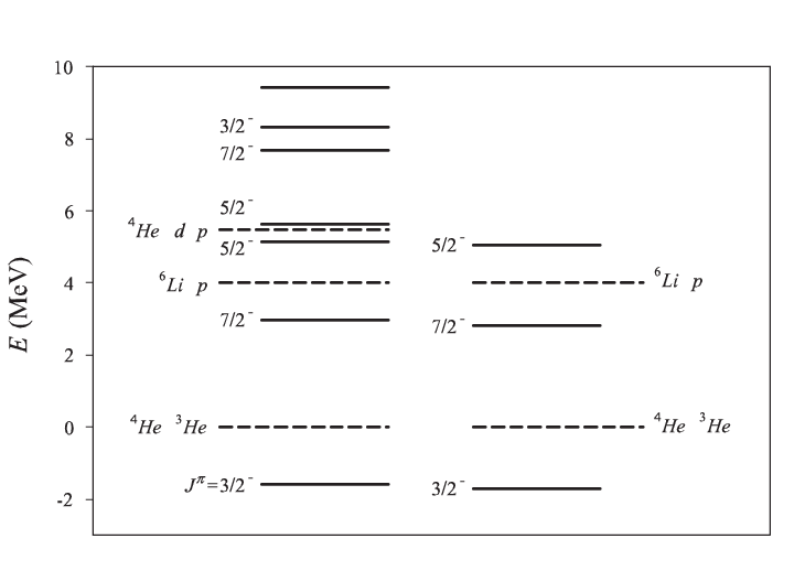
We now turn to the effect of the polarization of the two-cluster subsystems ${}^{6}Li$ and ${}^{3}He$ on the ground state energy of ${}^{7}Be$. We do so comparing results with ( marked ”Y”) and without (marked ”N”) polarization of the subsystem in Table 4. We suppress the polarization by using only a single function instead of all eigenfunctions of the corresponding two-cluster hamiltonian in the calculations. This corresponds to a rigid cluster throughout the calculation, whereas using the full set of eigenfunctions allows for adapting the size and shape of the subsystem to the presence of the third cluster. One notices that the polarization of ${}^{6}Li$ has a stronger impact than that of ${}^{3}He$.

Using the same (Y,N) approach we look at the effect of cluster polarization on the phase shift of ${}^{4}He+^{3}He$ elastic scattering with total momentum $J^{\pi}=7/2^{-}$ ($L=3$) in Fig. 3.

Similarly, in table 5 we look at the effect on the parameters for the 7/2^- and 5/2^- resonance states.

The cluster polarization substantially decreases the resonance energy and width, which points to an increase in the effective interaction between the clusters. The same observation has been made in [7, 8, 9, 10, 11, 13, 14, 48] for collective monopole and quadrupole polarizations. One again notices that the polarization of the ${}^{6}Li$ cluster is more important than that of the of ${}^{3}He$ cluster. The resonance properties, obtained with ${}^{6}Li$ polarization are only marginally different from those calculated with both ${}^{6}Li$ and ${}^{3}He$ polarizations.

The electromagnetic observables can calculated using the explicit ground state wave function. In Table 6 we list root-mean-square radii (proton ($R_{p}$), neutron ($R_{n}$) and mass ($R_{m}$)) and the quadrupole moments (proton ($Q_{p}$), neutron ($Q_{n}$) and mass ($Q_{m}$)) for the 3/2^- ground state. As one expects, the proton radius is larger than the neutron one. The quadrupole moment is an indicator of the deformation of the nucleus, and a negative value corresponds to a prolate deformation. The differences in these moments reflect the pronounced cluster structure of the ${}^{7}Be$ ground state.

In Table 6 we compare our GOB results with those of the multi-channel RGM of Arai et al (MCRGM) [16]), of the single-channel RGM of Kajino et al. (SCRGM) [25]), of the Stochastic Variational Method (SVM) [36] and of the Shell Model (SM) calculations [59].

The GOB results are close to those of SVM [36], and of the multi-channel RGM [16]. These results have also obtained with the MP interaction.

The single-channel SCRGM results of [25] have been obtained with the modified Hasegawa-Nagata potential. The ground state quadrupole moment is comparable, whereas the charge radius is much larger in the SCRGM.

The Shell Model calculation of [59] has been performed with the Bonn nucleon-nucleon potential. Its results for the charge radius and quadrupole moments are smaller than in the cluster models (MCRGM, SCRGM, SVM,GOB). This can be attributed to the fact that the Shell Model, involving a $10\hbar\Omega$ or $12\hbar\Omega$ state space, confines the inter-cluster distances in the ${}^{7}Be$ nucleus. In comparison, the GOB model uses a model space of $200\hbar\Omega$ for the inter-cluster behavior of the dominant ${}^{4}He+^{3}He$ cluster configuration.

As discussed in the introduction, one can distinguish collective polarization (quadrupole and monopole) for the compound nucleus as a whole (QM), RGM models with monopole excitations of the individual clusters (MRGM), and cluster polarization as described in the GOB model. It is interesting to compare these different polarization methods to gauge their impact on the ground state energy.

A detailed study in MRGM is only available for ${}^{7}Li$ [61], so we investigate the three methods applied to this nucleus, as it should have deformation properties comparable to ${}^{7}Be$.

To make the comparison consistent, we use the MP interaction parameters of [61], i.e. $u=1.0174$ and a spin-orbital strength of 0.821 (it is 1.0 for the other calculations in this paper, as suggested in [56]). With this interaction, we have performed the QM calculations along the lines reported in [15] and [14], a GOB calculations for a single $\alpha+t$ channel (SGOB) and a full GOB calculation as outlined in this paper. A standard RGM calculation without cluster polarization (SRGM) has been included as a benchmark.

In Table 7 the results for the different polarization models are displayed. One notices that the collective QM and SGOB models, which are comparable in terms of model space, improve with respect to the MRGM that includes only monopole cluster polarization. Clearly the full GOB calculation (including cluster polarization of ${}^{6}Li$ in the ${}^{6}Li+n$ channel) provides the best results. This was to be expected from the above ${}^{7}Be$ results.

We notice that in the MRGM calculation, the monopole polarization of ${}^{3}He$ is obtained by using four Gaussian functions resulting in -5.906 MeV of binding energy. In the SGOB model four Gaussian cluster functions are used to describe cluster polarization of ${}^{3}He$, and yields a binding energy of -5.953 MeV. This confirms the above results.

We can thus state that the cluster polarization of the channel subsystems described in the GOB model indeed plays an important role in seven-nucleon systems, and currently represents most prominent polarization type.

The expansion coefficients $\left\{C_{\nu_{\alpha}\lambda_{\alpha};n_{\alpha}l_{\alpha}}^{\left(\alpha\right)}\right\}$ determine the three-cluster wave function $\Psi^{J}$ (8) and also the Faddeev components $f_{\alpha}\left(\mathbf{x}_{\alpha},\mathbf{y}_{\alpha}\right)$ ($\alpha=1,2,3$) (4). We use the latter representation to analyze the wave function.

The correlation function for the ground state is

where the integration runs over the unit vectors $\widehat{\mathbf{x}}_{\alpha}$ and $\widehat{\mathbf{y}}_{\alpha}$.

To interpret the the polarizability in terms of the three-cluster structure, we introduce the root-mean-square radii $R_{\alpha}$:

and

They represent the root-mean-square radius of a two-cluster subsystem as a function of its distance to the third cluster (i.e. the distance of the centre-of-mass of the two-cluster system to the centre-of-mass of the third cluster).

We introduce new coordinates $\mathbf{r}_{\alpha}$ and $\mathbf{S}_{\alpha}$ whose norms ($r_{\alpha}$ and $S_{\alpha}$ correspond to the distances between the centers of mass of the clusters, that allow for a proper interpretation of the quantities (36) and (37). They relate to the original Jacobi coordinates as:

Fig. 4 displays the correlation function for the ${}^{4}He+^{3}He$ channel and Fig. 5 for the ${}^{6}Li+p$ channel. One notices from Fig. 4 that the distance between ${}^{4}He$ and ${}^{3}He$ is approximately 8 fm, and much larger than the separation of $d$ and $p$. From Fig. 5 one observes that the binary cluster configuration ${}^{6}Li+p$ is surprisingly compact. Both the distance between ${}^{4}He$ and $d$ and between ${}^{6}Li$ and $p$ are around 1 fm. These different geometric configurations can be related to the ground state energy relative to the thresholds of the corresponding binary channel. Indeed, the ground state is positioned at -$1.702$ MeV from the ${}^{4}He+^{3}He$ threshold and at -$5.722$ MeV with from the ${}^{6}Li+p$ threshold. This agrees with a very dispersed ${}^{4}He+^{3}He$ and a compact ${}^{6}Li+p$ configuration.

In Fig. 6 we show the dependence of the root-mean-square radius of the two-cluster subsystems on the distance from the third cluster. One notices how ${}^{6}Li$ strongly adapts its size when the proton is at large distances (more than 15 fm) from ${}^{6}Li$. When the ${}^{6}Li$ and the proton are near,the ${}^{6}Li$ $0^{+}$ ground state gets compressed approximately 1.5 times, and the $2^{+}$ excited state approximately two times. The ${}^{3}He$ nucleus, in a two-cluster configuration $d+p$, is strongly affected when the $\alpha$-particle is closer than 6 to 7 fm. Note that without polarization all three curves in Fig. 6 would be horizontal lines, as the two-cluster subsystems then have a constant size. The figure illustrates the impact of cluster polarization of ${}^{6}Li$ and ${}^{3}He$ in the description of ${}^{7}Be$.

The astrophysical $S$-factor of the reaction ${}^{6}Li\left(p,^{3}He\right)^{4}He$ is obtained from the total cross section, which has been computed with four total angular momentum $L=0$, $1$, $2$ and $3$. We have observed that zero angular momentum contribution dominates the low energy range $0\leq E\leq 1$ MeV of the cross section.

Fig. 7 displays the $S$-factor of the ${}^{6}Li\left(p,^{3}He\right)^{4}He$ reaction calculated for $L=0$. In contrast to the analysis of the ground state and resonance energies, the effects of cluster polarization are less evident here. In Fig. 7 it is seen that ${}^{3}He$ polarization increases the $S$-factor, thus increasing the coupling between the channels. The ${}^{6}Li$ polarization only has a small effect on the $S$-factor.

References

- [1] D. J. Stubeda, Y. Fujiwara, and Y. C. Tang, Phys. Rev. C 26 (1982) 2410.
- [2] H. Kanada, T. Kaneko, and Y. C. Tang, Phys. Rev. C 38 (1988) 2013.
- [3] H. Kanada, T. Kaneko, and Y. C. Tang, Nucl. Phys. A 380 (1982) 87.
- [4] H. Kanada, T. Kaneko, and Y. C. Tang, Nucl. Phys. A 389 (1982) 285.
- [5] H. Kanada, T. Kaneko, M. Nomoto, and Y. C. Tang, Prog. Theor. Phys. 72 (1984) 369.
- [6] H. Kanada, T. Kaneko, P. N. Shen, and Y. C. Tang, Nucl. Phys. A 457 (1986) 93.
- [7] G.F. Filippov, V.S. Vasilevsky, and A.V. Nesterov, Sov. J. Nucl. Phys. 40 (1984) 901.
- [8] E. Deumens, Nucl. Phys. A 423 (1984) 52.
- [9] G.F. Fillipov, V.S. Vasilevsky, and A.V. Nesterov, Bull. Acad. Sci. USSR, Phys. Ser. 48 (1984) 91.
- [10] G. F. Filippov, V. S. Vasilevsky, and L. L. Chopovsky, Sov. J. Part. and Nucl. 16 (1985) 153.
- [11] G.F. Filippov, V.S. Vasilevsky, M. Bruno, F. Cannata, M. D’Agostino, and F. Ortolani, Sov. J. Nucl. Phys. 51 (1990) 978.
- [12] G. F. Filippov, V. S. Vasilevsky, and A. V. Nesterov, Nucl. Phys. A 426 (1984) 327.
- [13] G.F. Filippov, V.S. Vasilevsky, S.P. Kruchinin, and L.L. Chopovsky, Sov. J. Nucl. Phys. 43 (1986) 536.
- [14] A. Sytcheva, F. Arickx, J. Broeckhove, and V. S. Vasilevsky, Phys. Rev. C 71 (2005) 044322.
- [15] A. Sytcheva, J. Broeckhove, F. Arickx, and V. S. Vasilevsky, J. Phys. G: Nucl. Part. Phys. 32 (2006) 2137.
- [16] K. Arai, D. Baye, and P. Descouvemont, Nucl. Phys. A 699 (2002) 963.
- [17] K. Arai, P. Descouvemont, and D. Baye, Phys. Rev. C 63 (2001) 44611.
- [18] Y. Fujiwara, Q. K. K. Liu, and Y. C. Tang, Phys. Rev. C 38 (1988) 1531.
- [19] Y. Fujiwara and Y. C. Tang, Phys. Rev. C 31 (1985) 342.
- [20] H. Walliser, H. Kanada, and Y. C. Tang, Nucl. Phys. A 419 (1984) 133.
- [21] T. Mertelmeier and H. M. Hofmann, Nucl. Phys. A 459 (1986) 387.
- [22] H. M. Hofmann, T. Mertelmeier, and W. Zahn, Nucl. Phys. A 410 (1983) 208.
- [23] H. Walliser, Q. K. K. Liu, H. Kanada, and Y. C. Tang, Phys. Rev. C 28 (1983) 57.
- [24] T. Kajino, Nucl. Phys. A 460 (1986) 559.
- [25] T. Kajino, T. Matsuse, and A. Arima, Nucl. Phys. A 413 (1984) 323.
- [26] E.G. Adelberger et al., Rev. Mod. Phys. 70 (1998) 1265.
- [27] A. Coc, C. Angulo, E. Vangioni-Flam, P. Descouvemont, and A. Adahchour, Nucl. Phys. A 752 (2005) 522.
- [28] A. Csótó, and K. Langanke Few-Body Syst. 29 (2000) 121.
- [29] P. Mohr, H. Abele, R. Zwiebel, G. Staudt, H. Krauss, H. Oberhummer, A. Denker, J. W. Hammer, and G. Wolf, Phys. Rev. C 48 (1993) 1420.
- [30] B. Buck, and A. C. Merchant, J. Phys. G: Nucl. Phys. 14 (1988) 211.
- [31] V. Vasilevsky, F. Arickx, J. Broeckhove, and V.N. Romanov, Proc. of 10th Int. Conference on Nuclear Reaction Mechanisms, Varenna, Italy, June 9 - 13 2003, (E.Gadioli, ed.), Milano, University of Milano, Ricerca Scientifica ed Educazione Permanente, Suppl. No. 122 (2003) 73.
- [32] V. Vasilevsky, F. Arickx, J. Broeckhove, and V. Romanov, Ukr. J. Phys. 49 (2004) 1053.
- [33] V. I. Kukulin and V. M. Krasnopolsky, J. Phys. G3 (1977) 795.
- [34] K. Varga, Y. Suzuki, and R. G. Lovas, Nucl. Phys. A 571 (1994) 447.
- [35] K. Varga and Y. Suzuki, Phys. Rev. A 53 (1996) 1907.
- [36] K. Varga, Y. Suzuki, K. Arai, and Y. Ogawa, Nucl. Phys. A 616 (1997) 383.
- [37] K. Varga and Y. Suzuki, Phys. Rev. C 52 (1995) 2885.
- [38] E. Hiyama, Y. Kino, and M. Kamimura, Progr. Part. Nucl. Phys. 51 (2003) 223.
- [39] G. F. Filippov and I. P. Okhrimenko, Sov. J. Nucl. Phys. 32 (1981) 480.
- [40] G. F. Filippov, Sov. J. Nucl. Phys. 33 (1981) 488.
- [41] E. J. Heller and H. A. Yamani, Phys. Rev. A 9 (1974) 1201.
- [42] E. J. Heller and H. A. Yamani, Phys. Rev. A 9 (1974) 1209.
- [43] H. A. Yamani and L. Fishman, J. Math. Phys. 16 (1975) 410.
- [44] H. A. Yamani, J. Math. Phys. 23 (1982) 83.
- [45] J. M. Bang, A. I. Mazur, A. M. Shirokov, Y. F.Smirnov, and S. A. Zaytsev, Ann. Phys. 280 (2000) 299.
- [46] V. S. Vasilevsky, and I. Yu. Rybkin, Sov. J. Nucl. Phys. 50 (1989) 411.
- [47] V. S. Vasilevsky and F. Arickx, Phys. Rev. A 55 (1997) 265.
- [48] G. F. Filippov, V. S. Vasilevsky, , and L. L. Chopovsky, Sov. J. Part. and Nucl. 15 (1984) 600.
- [49] V. Vasilevsky, A. V. Nesterov, F. Arickx, and J. Broeckhove, Phys. Rev. C 63 (2001) 034606.
- [50] L. D. Faddeev and S. P. Merkuriev, Quantum Scattering Theory for Several Particle Systems. Dordrecht, Boston, London: Kluwer Academic Publishers, 1993.
- [51] V. Vasilevsky, F. Arickx, and J. Broeckhove, J. Phys. Conf. Ser. 111 (2008) 2055.
- [52] W. Tobocman, Theory of direct nuclear reactions. Oxford University Press, London, 1961.
- [53] N. Austern, Direct Nuclear Reaction Theories. Wiley-Interscience, New York, 1970.
- [54] R. F. Barrett, B. A. Robson, and W. Tobocman, Rev. Mod. Phys. 55 (1983) 155.
- [55] D. R. Thompson, M. LeMere, and Y. C. Tang, Nucl. Phys. A 268 (1977) 53.
- [56] I. Reichstein, and Y. C. Tang, Nucl. Phys. A 158 (1970) 529.
- [57] D. R. Tilley, C. M. Cheves, J. L. Godwin, G. M. Hale, H. M. Hofmann, J. H. Kelley, C. G. Sheu, and H. R. Weller, Nucl. Phys. A 708 (2002) 3.
- [58] K. Varga, Y. Suzuki, and Y. Ohbayasi, Phys. Rev. C 50 (1994) 189.
- [59] P. Navratil, C. A. Bertulani, and E. Caurier, Phys. Lett. B 634 (2006) 191.
- [60] I. Tanihata, H. Hamagaki, O. Hashimoto, Y. Shida, N. Yoshikawa, K. Sugimoto, O. Yamakawa, T. Kobayashi, and N. Takahashi, Phys. Rev. Lett. 55 (1985) 2676.
- [61] T. Kaneko, M. Shirata, H. Kanada, and Y. C. Tang, Phys. Rev. C 34 (1986) 771.
- [62] J. B. Marion, G. Weber, and F. S. Mozer, Phys. Rev. 104 (1956) 1402.
- [63] U. Fasoli, D. Toniolo, and G. Zag, Phys. Lett. 8 (1964) 127.
- [64] W. Gemeinhardt, D. Kamke, and C. von Rh�neck, Z. Phys. 97, p. 58, (1966).
- [65] O. Fiedler and P. Kunze, Nucl. Phys. A 96 (1967) 513.
- [66] H. Spinka, T. Tombrello, and H. Winkler, Nucl. Phys. A 164 (1971) 1.
- [67] C. R. Gould, R. O. Nelson, J. R. Williams, and J. R. Boyce, Nucl. Sci. Eng. 55 (1974) 267.
- [68] C.-S. Lin, W.-S. Hou, M. Wen, and J.-C. Chou, Nucl. Phys. A 275 (1977) 93.
- [69] A. J. Elwyn, R. E. Holland, C. N. Davids, L. Meyer-Schutzmeister, F. Mooring, and W. R. Jr, Phys. Rev. C 20 (1979) 1984.
- [70] S. Engstler, G. Raimann, C. Angulo, U. Greife, C. Rolfs, U. Schröder, E. Somorjai, B. Kirch, and K. Langanke, Phys. Lett. B 279 (1992) 20.
- [71] C. Angulo, M. Arnould, M. Rayet, P. Descouvemont, D. Baye, C. Leclercq-Willain, A. Coc, S. Barhoumi, P. Aguer, C. Rolfs, R. Kunz, J. W. Hammer, A. Mayer, T. Paradellis, S. Kossionides, C. Chronidou, K. Spyrou, S. degl’Innocenti, G. Fiorentini, B. Ricci, S. Zavatarelli, C. Providencia, H. Wolters, J. Soares, C. Grama, J. Rahighi, A. Shotter, and M. Lamehi Rachti, Nucl. Phys. A 656 (1999) 3.