$A$ dependence of the enhancement factor in energy-weighted sums for isovector giant resonances

A microscopic description of the isovector excitations within the nuclear Fermi-liquid theory requires the use of two Landau amplitudes $F_{0}^{\prime}$ and $F_{1}^{\prime}$ to model the nucleon-nucleon interaction. The amplitude $F_{0}^{\prime}$ provides the isospin symmetry energy, whereas the inclusion of the velocity-dependent force $\sim F_{1}^{\prime}$ leads to the renormalization of the isovector energy weighted sums (EWS) $m_{k}$ [1, 2]. In particular, the isovector EWS $m_{1}$ becomes dependent on the nucleon-nucleon interaction. This is opposite to the case of the isoscalar excitations where the corresponding sum $m_{1}$ is model independent. Moreover, the presence of the velocity dependent force gives rise to an exceed of the $100\%$ exhaustion of Thomas-Reiche-Khun (TRK) sum rule for the isovector giant dipole resonances (IVGDR). The origin of the corresponding enhancement factor of the IVGDR sum $m_{1}$ was intensively investigated for both the nuclear matter and the finite nuclei, see Refs. [1, 3] and references therein. The RPA calculations of the enhancement factor for the symmetric nuclear matter were recently performed for a representative set of Skyrme forces in Ref. [4]. As shown in [4], the value of the enhancement factor is changed in almost 2 times depending on the choice of the Skyrme force parametrization. The high sensitivity of the enhancement factor to the choice of the Skyrme forces was also demonstrated in Ref. [5] for the nucleus ²⁰⁸Pb.

In finite nuclei, both the IVGDR eigenenergy $E_{\mathrm{IVGDR}}$ and the EWS $m_{1}$ are rather complicated functions of the mass number $A$. In contrast to the classical Steinwedel-Jensen model [6], the value $E_{\mathrm{IVGDR}}\cdot A^{1/3}$ is not a constant but increases with $A$. The theoretical approaches to microscopic description of IVGDR are mainly based on the Random Phase Approximation (RPA) [7]. The RPA analysis of the enhancement factor for some spherical nuclei (but not its $A$-dependence) has been recently done in Ref. [8]. Note, however, that the RPA calculations [1, 3, 8, 9] overestimate the magnitude of the enhancement factor, see below Figure 3. Note also, that within the RPA, the highly excited IVGDR is strongly fragmented over a wide energy interval and a special averaging procedure has to be applied to pick up a smooth $A$-dependence of the IVGDR characteristics. Furthermore, the RPA calculations of the EWS $m_{k}$ are restricted due to taking into account $1p-1h$ excitations only and, thereby, one can expect an underestimation of the contribution to $m_{1}$ from more complicated states [1, 10, 9, 11].

In this work, we study the IVGDR within the Landau kinetic theory [12], that is extended to the finite two-component Fermi-liquid drop. The $A$-dependence of both the IVGDR eigenenergy and the corresponding EWS occurs due to the boundary conditions on the moving nuclear surface. Our approach is more general than the scaling model [13] or the fluid dynamic approaches [14] due to the fact that it takes into consideration all multipolarities of the Fermi surface distortions.

In Sect. II, we start from the response theory based on the collisionless kinetic Landau-Vlasov approach to the isovector excitations. We derive the main characteristics of the IVGDR, taking into account the velocity dependent part of the Landau isovector interaction. In Sect. III, we obtain the boundary condition for the isovector sound mode on the free nuclear surface. In Sect. IV, the numerical calculations for the IVGDR eigenenergy and the corresponding EWS sum $m_{1}$ are presented. Conclusions are given in Sect. V.

We consider the response of the nucleus to an external periodic in time field $U_{\mathrm{ext}}(t)$:

where $\hat{q}$ is the Hermitian one-particle operator, which depends on both spatial and isospin coordinates. If we assume $\lambda_{0}\ll 1$, the quantum mechanical expectation of the operator $\hat{q}$ is given by the following form [15]

where $\chi(\omega)$ is the linear response function. We will evaluate the isovector density-density response function $\chi(\omega)$ by using

where $\tau_{j}=1$ for the neutron and $\tau_{j}=-1$ for the proton.

To evaluate the response function $\chi(\omega)$, we use the collisionless kinetic Landau-Vlasov equation for the isovector excitations

Here, $\delta{f}$ is the isovector variation of the Wigner distribution function, $\vec{v}$ is the nucleon velocity, $f_{\mathrm{eq}}$ is the equilibrium distribution function and $\delta{U}_{\mathrm{self}}$ describes the dynamical component of the selfconsistent mean field.

The solution to Eq. (3) can be written in terms of a plane wave [12]

where $\varepsilon_{p}=p^{2}/2m^{\ast}$, $m^{\ast}$ is the nucleon effective mass and $\nu_{\vec{q}}(\vec{p})$ is an unknown amplitude. The variation of the self-consistent field $\delta U_{\mathrm{self}}$ in Eq. (3) is obtained through the isovector interaction amplitude $F^{\prime}(\vec{p},\vec{p}^{\prime})$ as

The interaction amplitude $F^{\prime}(\vec{p},\vec{p}^{\prime})$ is usually parametrized in terms of the Landau constants $F_{k}^{\prime}$ as [16]

where $P_{k}(x)$ is the Legendre polynomial, $N_{F}$ is the averaged density of states at the Fermi surface, given by

and $p_{F}$ is the Fermi momentum.

The parameter ${F}_{0}^{\prime}$ is related to the isotopic symmetry energy $C_{\mathrm{sym}}$ in the Weizsäcker mass formula [6, 16]

with the Fermi energy $\varepsilon_{F}=p_{F}^{2}/2m^{\ast}$. In the following, we will assume that

By using Eq. (3) to get the amplitudes $\nu_{\vec{q}}(\vec{p})$, we obtain the isovector response function in the form [17]

Here, $s=\omega m^{\ast}/qp_{F}$,

and

The frequencies of isovector eigenvibrations [the poles of the response function (10)] can be derived from the dispersion relation

The response function in Eq. (10) allows us to evaluate the isovector EWS

Using the dispersion relation between $\mathrm{{Im}{\chi}(\omega)}$ and $\mathrm{{Re}{\chi}(\omega)}$, and the asymptotic behavior of $\mathrm{{Re}{\chi}(\omega)}$ at $\omega\rightarrow 0$ and $\omega\rightarrow\infty$ limits, one obtains (see also Ref. [1])

Here, we introduced the renormalized (because of the Fermi surface distortion effect) isotopic symmetry energy $C_{\mathrm{sym}}^{\prime}=C_{\mathrm{sym}}+8\varepsilon_{F}/15$ and the effective mass $m^{\prime}=m/(1+\kappa_{NM})$ for the isovector channel, where $\kappa_{NM}$ is the enhancement factor of the sum rule (for nuclear matter), which is defined by the relation

where $F_{k}$ is the Landau amplitude for the isoscalar channel. In contrast to the isoscalar excitations, the isovector EWS sum ${m}_{1}$ in Eq. (15) is not model independent in the sense that it depends on the effective mass ${m}^{\prime}$ and, thereby, on the interaction amplitudes $F_{1}$ and ${F}_{1}^{\prime}$. We also point out that the EWS ${m}_{k}$ of Eq. (15) allows us to evaluate the constrained energy, $E_{\mathrm{constr}}$, and the scaling energy, $E_{\mathrm{sc}}$, for the IVGDR. Namely,

For finite nuclei, the dispersion relation [Eq. (13)] has to be supplemented by a corresponding boundary condition. The boundary condition can be viewed as a condition for a balance of the forces acting on the free nuclear surface

where $\vec{n}$ is the unit vector normal to the nuclear surface $S$, the internal force $\vec{F}$ is associated with the isovector sound wave and $\vec{F}_{S}$ is the isovector surface tension force. The internal force $\vec{F}$ is defined by the momentum flux tensor $\delta P_{\alpha\beta}$ inside the nuclear volume. Thus, $F_{\alpha}=n_{\beta}\delta P_{\alpha\beta}$ where $\delta P_{\alpha\beta}$ is given by [18, 19]

Here, $\vec{\xi}$ is the displacement field, $\bar{\rho}_{\mathrm{eq}}=(\rho_{n,\mathrm{eq}}+\rho_{p,\mathrm{eq}})/2$, and

The surface force $\vec{F}_{S}$ in Eq. (18) is defined as $F_{\nu,S}=n_{\nu}\delta P_{S}$, where $\delta P_{S}$ is the pressure caused by the isovector polarizations at the nuclear surface [13, 17], given by

Here, $r_{0}$ is the mean distance between nucleons, $Q$ is related to the surface symmetry energy in the Weizsäcker mass formula [20] and $\delta R_{1}=R_{0}\alpha_{S}(t)Y_{10}(\hat{r})$. The amplitude $\alpha_{S}(t)$ of the isovector vibrations of the nuclear surface is connected to the corresponding amplitude $\vec{\xi}$ of the displacement field in a sound wave.

Finally, from Eqs. (18), (19) and (21) we derive the following secular equation for the wave number $q$

where $x=qR_{0}$ and $R_{0}=r_{0}A^{1/3}$. In the limit $Q\rightarrow\infty$, the boundary condition [Eq. (22)] gives rise to the boundary condition $j_{1}^{\prime}(x)=0$ of the Steinwedel-Jensen model [6]. We point out that the secular equation (22) for $q$ has to be solved consistently with the dispersion equation (13) for $s$.

Numerical calculations were carried out by using the following set of nuclear parameters: $r_{0}=1.2$ fm, $F_{1}=-0.3$ and $F_{0}^{\prime}=1.41$. According to Eq. (8), the bulk symmetry energy $C_{\mathrm{sym}}$ is equal to $60$ MeV [6]. The value of the Landau amplitude $F_{1}^{\prime}$ will be discussed in the following.

In Figure 1, the solid curve 1 shows the $A$ dependence of the value $x$ obtained from the secular equation (22); it is consistent with the dispersion relation [Eq. (13)] including all multipolarities $l$ of the Fermi surface distortions. Curve 3 represents the analogous result but for the velocity-independent nuclear forces (i.e., for $F_{1}=0$ and $F_{1}^{\prime}=0$). Curve 2 shows a solution to the secular equation (22), when one takes into account the Fermi surface distortions up to quadrupole order (scaling approximation with $l\leq 2$) [13]. In the last case, instead of solving the dispersion equation (13), we have used the expression $s^{2}=(9/5+F_{0}^{\prime})/3$, which gives the dimensionless sound velocity $s$ for $l\leq 2$ [19]. As seen from Figure 1, the value of $x$ is significantly smaller than the corresponding one obtained within the Steinwedel-Jensen model (dashed line in Figure 1).

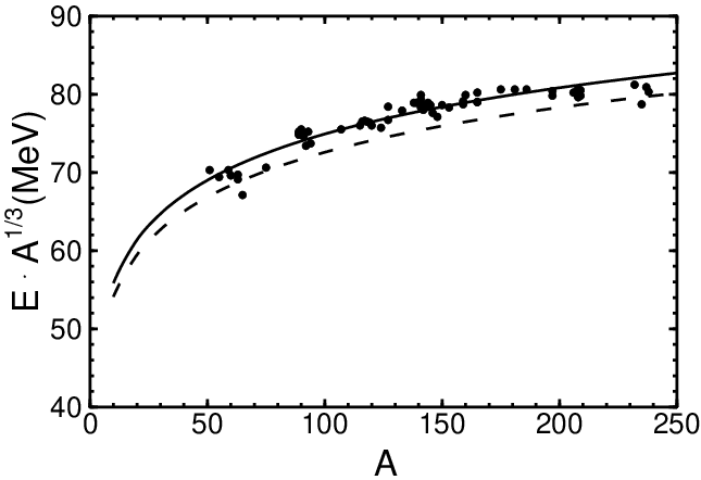
In Figure 2 we show a dependence of the IVGDR energy (multiplied by the factor $A^{1/3}$) on the mass number $A$. The calculations have been performed at $Q=10.5$ MeV and $F_{1}^{\prime}=1.1$. The solid line is the eigenenergy obtained from the dispersion equation (13) supplemented by the boundary condition [Eq. (22)]. The dashed line in Figure 2 was obtained from the EWS definition of the scaling energy, $E_{\mathrm{sc}}$, of Eq. (17). A significant upward shift of the exact eigenenergy (solid line) with respect to the scaling one, $E_{\mathrm{sc}}$, is due to the Fermi surface distortions of the higher multipolarities ($l>2$) contributed to the dispersion equation (13). The values of the Landau amplitude $F_{1}^{\prime}=1.1$ and the parameter $Q=10.5$ MeV have been chosen such that the best fit of the $A$ dependence of the eigenenergies to the experimental data is obtained.

Let us now consider the enhancement factor $\kappa$ of the isovector EWS $m_{1}$. For infinite nuclear matter, it is given by the value of $\kappa_{NM}$ in Eq. (16). The experimental determination of the enhancement factor $\kappa$ is connected to the investigation of the photoabsorption cross section $\sigma_{\mathrm{abs}}(\omega)$ of $\gamma$ quanta. For the velocity-independent forces, the isovector EWS $m_{1}$ is model independent and reads (TRK sum rule) [7]

The photoabsorption cross section $\sigma_{\mathrm{abs}}(\omega)$ can be expressed in terms of the strength function $S(\omega)=\mathrm{{Im}{\chi}(\omega)/\pi}$ as follows [21]:

where the wave number $q_{0}(A)$ has to be found from Eq. (22) in the limit of velocity-independent forces, i.e., at $F_{1}=0$ and $F_{1}^{\prime}=0$.

In a general case of velocity-dependent nuclear forces, by using Eq. (15) for $m_{1}$ and Eqs. (23) and (24), we generalize the TRK sum rule in the form

where $q_{1}(A)$ is derived by Eq. (22) at $F_{1}\neq 0$ and $F_{1}^{\prime}\neq 0$.

In Figure 3, the EWS enhancement factor $1+\kappa(A)$ is plotted as a function of the mass number $A$:

The exceedance of the $100{\%}$ sum rule for $\widetilde{m}_{1}(A)$, which is observed for the IVGDR, is caused by the dependence of the effective nucleon-nucleon interaction on the nucleon velocity. For the value of the isovector amplitude $F_{1}^{\prime}=1.1$, one can fit (on average) the results of our calculations of $1+\kappa(A)$ (solid curve in Figure 3) to the experimental data of the Livermore group [22]. Our estimate to the enhancement factor $\kappa(A)$ is about $10\%$ for light nuclei and increases to $20\%$ for heavy nuclei. This result is consistent with the general conclusion of Ref. [22]; that is, for $A>100$, the experimental data center is at about $1.2$ TRK sum-rule units. For the mass region $A<70$, the TRK sum rule is not exhausted. As noted in Ref. [22], this no doubt results from the neglect of the $(\gamma,p)$ channel contribution for these nuclei. It was reported recently that inclusion of the contribution from the $(\gamma,p)$ cross section increases the EWS exhaustion from $0.87$ to $1.15$ for ⁶⁰Ni and from $0.64$ to $0.92$ for ⁶³Cu [23]. The corresponding new data are shown in Figure 3 by the symbol $\star$. The result of a microscopic RPA calculation of the enhancement factor is shown in Figure 3 as a dashed line (see Refs. [1, 10]). We point out that both our Fermi-liquid approach and the RPA prediction give very similar $A$ dependence of the enhancement factor $1+\kappa(A)$. However, it is seen from Figure 3 that the RPA calculation overestimates the magnitude of $\kappa(A)$ (see also Refs. [3, 9, 8]). The RPA result for $\kappa(A)$ can be improved by a fit of the relevant parameters $t_{1}$ and $t_{2}$ in the Skyrme forces.

The corresponding study has been recently performed within the microscopic Hartree-Fock plus RPA approach in Ref. [5], where a best value for $\kappa(A)$ of $0.22\pm 0.04$ was deduced from a fit to the experimental data for the nucleus ²⁰⁸Pb. However, reducing the enhancement factor by the variation of the Skyrme force parameters, one can expect a significant change of the $A$ behavior (slope) of the corresponding curve $\kappa(A)$ (dashed line in Figure 3). Unfortunately, in the nuclear literature, this kind of analysis has not yet been carried out. We also note that the latest microscopic RPA calculations presented in Refs. [4, 5] are related to nuclear matter and the nucleus ²⁰⁸Pb only. They do not show an $A$ dependence of the enhancement factor, but they do give a demonstration of significant variation of the dependence of the enhancement factor on the choice of the Skyrme force parametrization (see the last column in Table I of Ref. [5]).

In conclusion, we wish to comment that it was conceptually important for us to achieve a description of the $A$ dependence of both the IVGDR energy and the enhancement factor simultaneously (see FIGs. 2 and 3). In our approach, we used appropriate boundary conditions that allowed us to combine both the Steinwedel-Jensen and Goldhaber-Teller models. A similar problem was considered earlier in Ref. [13] but within the scaling approximation only. Thus, an inclusion of the effective isovector surface stiffness $Q$ into the boundary condition [Eq. (22)] leads to the $A$ dependence of the value $qR_{0}$, which becomes significantly smaller than the Steinwedel-Jensen’s estimate $qR_{0}=2.08$ [6]. Using the obtained value of $qR_{0}$, we have described the IVGDR energies within the Landau kinetic theory quite well. Fitting the slope of the energy dependence on the mass number $A$ to the experimental data, we have estimated the value of the effective isovector surface stiffness as $Q\simeq 11$ MeV.

The dependence of the effective nucleon-nucleon interaction on the nucleon velocity causes the $100{\%}$ exhaustion of the TRK sum rule to be exceeded for the IVGDR. Within Landau kinetic theory, the EWS enhancement factor $\kappa_{NM}$ in infinite nuclear matter depends on the interaction amplitudes $F_{1}$ and $F_{1}^{\prime}$. In finite nuclei, the $A$ dependence of the EWS enhancement factor $\kappa(A)$ occurs because of the boundary condition [Eq. (22)]. The value of $\kappa(A)$ increases with $A$. A fit of the enhancement factor to the proper experimental data leads to a value for the isovector Landau amplitude of $F_{1}^{\prime}\simeq 1.1$. The obtained value of $F_{1}^{\prime}$ exceeds the estimate $F_{1}^{\prime}=0.5-0.7$ derived earlier from Skyrme forces for infinite nuclear matter [9, 11, 16]. This exceedance appears since our derivation of $F_{1}^{\prime}$ is related to the interior of the finite nucleus. For finite nuclei, the Landau amplitudes $F_{k}$ and $F_{k}^{\prime}$ are $r$-dependent ones with a bump within the nuclear surface [11, 16]. This effectively increases the bulk values of $F_{k}$ and $F_{k}^{\prime}$ in the limit of the sharp nuclear surface assumed in this paper.

We show that the value of the enhancement factor is about $10\%$ for light nuclei and reaches approximately $20\%$ for heavy nuclei. For nuclei with $A>100$, our results are close to the experimental data from Livermore discussed in Ref. [22] and they are in agreement with the best value for the enhancement factor obtained for the nucleus ²⁰⁸Pb in Ref. [5]. We note also that the $A$ behavior of the enhancement factor obtained in our Fermi-liquid approach is similar to the one derived from the microscopic RPA calculations (see dashed line in FIG. 3), but, as was previously mentioned, the RPA results show a strong variation of the enhancement factor with the choice of the Skyrme force parametrization [5].

References

- [1] E. Lipparini and S. Stringari, Phys. Rep. 175, 103 (1989).
- [2] I. Hamamoto, H. Sagawa and X. Z. Zhang, Nucl. Phys. A649, 319 (1999).
- [3] M. Traini, G. Orlandini and R. Leonardi, Riv. Nuovo Cimento 10, 1 (1987).
- [4] V. O. Nesterenko, W. Kleinig, J. Kvasil, P. Vesely, and P.-G. Reinhard, Int. J. Mod. Phys. E 17, 89 (2008).
- [5] L. Trippa, G. Coló, and E. Vigezzi, Phys. Rev. C 77, 061304(R) (2008).
- [6] A. Bohr and B. Mottelson, Nuclear Structure, Vol. 2 (Benjamin, New York, 1975).
- [7] P. Ring and P. Schuck, The Nuclear Many-Body Problem (Springer-Verlag, New York, 1980).
- [8] D. Sarchi, P. F. Bortignon, and G. Coló, Phys. Lett. B601, 27 (2004).
- [9] H. Krivine, J. Treiner and O. Bohigas, Nucl. Phys. A336, 155 (1980).
- [10] M. Beiner, H. Flocard, Nguen van Giai and P. Quentin, Nucl. Phys. A238, 29 (1975).
- [11] K. -F. Liu, H. Luo, Z. Ma, Q. Shen and S. A. Moszkowski, Nucl. Phys. A534, 1 (1991).
- [12] A. A. Abrikosov and I. M. Khalatnikov, Rep. Prog. Phys. 22, 329 (1959).
- [13] S. Stringari, Ann. Phys. 151, 35 (1983).
- [14] G. Holzwarth and G. Eckart, Nucl. Phys. A325, 1 (1979); H. Koch, G. Eckart, B. Schwesinger and G. Holzwarth, Nucl. Phys. A373, 173 (1982).
- [15] E. M. Lifshitz and L. P. Pitaevsky, Statistical Physics, Part 1 (Nauka, Moscow, 1976).
- [16] A. B. Migdal, Theory of Finite Fermi Systems and Applications to Atomic Nuclei (Interscience, London, 1967).
- [17] V. M. Kolomietz, S. V. Lukyanov, and O.O. Khudenko, Ukr. Phys. J. 52, 546 (2007).
- [18] V. M. Kolomietz and S. Shlomo, Phys. Rep. 390, 133 (2004).
- [19] A. Kolomiets, V. M. Kolomietz, and S. Shlomo, Phys. Rev. C 59, 3139 (1999).
- [20] W. D. Myers and W. J. Swiatecki, Ann. Phys. 84, 186 (1974).
- [21] M. Di Toro, V. M. Kolomietz, and A. B. Larionov, Phys. Rev. C 59, 3099 (1999).
- [22] B. L. Berman and S. C. Fultz, Rev. Mod. Phys. 47, 713 (1975).
- [23] O. A. Bezshyyko, L. O. Golinka-Bezshyyko, I. M. Kadenko, O. O. Kochergina, and O. S. Shashko, Nucl. Phys. and Atom. Energ. 4, 72 (2007).