GeV Emission from Prompt and Afterglow Phases of Gamma-Ray BurstsNote: August 6, 2007; revised June 30, 2008; accepted August 11, 2008
Abstract
We investigate the GeV emission from gamma-ray bursts (GRBs), using the results from the Energetic Gamma Ray Experimental Telescope (EGRET), and in view of the Gamma-ray Large Area Space Telescope (GLAST). Assuming that the conventional prompt and afterglow photons originate from synchrotron radiation, we compare an accompanying inverse-Compton component with EGRET measurements and upper limits on GeV fluence, taking Klein-Nishina feedback into account. We find that EGRET constraints are consistent with the theoretical framework of the synchrotron self-Compton model for both prompt and afterglow phases, and discuss constraints on microphysical parameters in both phases. Based on the inverse-Compton model and using EGRET results, we predict that GLAST would detect GRBs with GeV photons at a rate yr-1 from each of the prompt and afterglow phases. This rate applies to the high-energy tail of the prompt synchrotron emission and to the inverse-Compton component of the afterglow. Theory predicts that in a large fraction of the cases where synchrotron GeV prompt emission would be detected by GLAST, inverse-Compton photons should be detected as well at high energies ( GeV). Therefore GLAST will enable a more precise test of the high-energy emission mechanism. Finally, we show that the contribution of GRBs to the flux of the extragalactic gamma-ray background measured with EGRET is at least 0.01% and likely around 0.1%.
Subject headings
gamma-rays: bursts — radiation mechanisms: non-thermalI. Introduction
Cosmological gamma-ray bursts (GRBs) have released a tremendous amount of energy in the past and present Universe. Their emission covers very wide range of frequencies: a highly variable prompt phase radiates 100 keV gamma rays, while a subsequent afterglow radiates radio to X-ray photons. It is likely that the bulk of these photons are emitted by gyration of relativistic electrons in magnetic fields—e.g., synchrotron radiation. The relativistic electrons are accelerated in either internal dissipation (for prompt emission) or external shocks (for afterglows). For reviews, see, Piran [41], Mészáros [28], Nakar [33].
GeV photons were detected as well from several GRBs by the Energetic Gamma Ray Experimental Telescope (EGRET) on board the Compton Gamma Ray Observatory (CGRO) [48, 50, 19, 49, 13]. The data are still not sufficient for us to firmly infer emission mechanisms of these GeV gamma rays, but the most promising mechanism is synchrotron self-Compton (SSC) scattering [27, 53, 54, 7, 34, 56, 47, 17, e.g.,]. This is because the relevant emission parameters such as the energy fraction of the GRB jets going to electrons () and magnetic fields () are relatively well measured from the afterglow spectra as well as light curves; the typical values are and [35, 55, e.g.,]. In the prompt emission, is similar or even higher, as evident from the high efficiency of this phase, while is not well constrained. Thus, there should be a significant inverse-Compton (IC) component accompanying the synchrotron radiation in both the afterglow and prompt emission. The luminosities of the synchrotron and IC are expected to be comparable as IC-to-synchrotron luminosity ratio is roughly given by , according to theory [47, e.g.,].
In this paper, we explore the GeV gamma-ray emission of GRBs in the context of SSC mechanism.11 1 Our analysis and conclusions are applicable also if the MeV and/or radio-X-ray afterglow emission mechanism is not synchrotron but another type of emission from relativistic electrons that gyrate in a magnetic field, such as jitter radiation [26]. Besides the several GRBs detected by EGRET, there are many others for which upper bounds on the fluence were obtained [14]. These 100 GRBs should also be compared with the predictions of SSC model, because the fluence upper limits in the EGRET energy band are comparable to the fluence of prompt emission collected by Burst And Transient Source Experiment (BATSE) instrument onboard CGRO. As the experimental bound is already strong, while theoretical models of SSC process predict a large fluence for the EGRET energy range, we derive meaningful constraints from EGRET data analysis on the physics of the high-energy emission mechanisms of GRBs. This approach is different from (and therefore complementary with) that in previous studies [e.g., 9, 3, 20, 15, 12, 32, 36, and references therein], where the prediction of gamma-ray flux relies only on theoretical models and sub-GeV observations. We instead use EGRET data in order to infer the GeV emission and constrain the theoretical models.
We use our results to predict the expected number of GRBs that would be detected by the Gamma-ray Large Area Space Telescope (GLAST). The GLAST satellite is equipped with the Large Area Telescope (LAT), which is an upgraded version of EGRET. Since revealing the high-energy emission mechanisms of GRBs are one of the important objectives of GLAST, our prediction should give a useful guideline. Finally, we apply our results to estimate the contribution of GRBs to the diffuse extragalactic gamma-ray background (EGB), which was also measured by EGRET [51, 52, see, however, Keshet, Waxman, & Loeb 22 for a subtle issue of Galactic foreground subtraction].
This paper is organized as follows. In § II, we summarize the predictions of SSC model for the prompt (§ II.1) and afterglow (§ II.2) phases. Section III is devoted for analysis of the GRB fluence data by EGRET, from which distributions of fluence in the GeV band are derived. We then use these distributions to argue prospects for GRB detection with GLAST in § IV, and implications for EGB from GRB emissions in § V. In § VI, we give a summary of the present paper.
II. Inverse-Compton model of high-energy emission
If the prompt and/or afterglow emission is due to synchrotron radiation from relativistic electrons (with Lorentz factor ), then there must be an accompanying IC component from the same electrons scattering off the synchrotron photons. The spectral shape of the IC emission is almost the same as the synchrotron radiation (shifted by ), and is expected to fall around the GeV range during both the prompt and afterglow phases. For , and assuming that there is no “Klein-Nishina suppression” and that the emitting electrons are fast cooling, the IC fluence is related to the synchrotron fluence simply through . Thus, assuming that the microphysics do not vary much from burst to burst, it is natural to assume proportionality between the synchrotron MeV fluence (observed by BATSE) and the GeV synchrotron plus IC fluence (observed by EGRET and in the future by GLAST):
| (1) |
where and are coefficients for the proportionality due to synchrotron and IC processes. Note that the synchrotron fluence in the GeV range can be extrapolated relatively easily, if we assume that the spectrum extends up to such high energies. Thus, we here focus on theoretical evaluation of the IC component. At first approximation, the coefficient is roughly from considerations above, and thus we define
| (2) |
where for the prompt emission while for the afterglow is the afterglow fluence within the radio to X-ray energy bands. Correction factors and represent the effect of Klein-Nishina suppression and detector energy window, respectively, which are given below.
We define typical frequencies for both synchrotron () and IC () as the frequencies where most of the energies are radiated in case that the Klein-Nishina cross section does not play an important role; i.e., where for each component is peaked in this case. From relativistic kinematics, these two typical frequencies are related through
| (3) |
where is a characteristic Lorentz factor of the electrons that dominate the synchrotron power [46]; this is true in the fast cooling regime, which is the case in the most of our discussions [47]. The Klein-Nishina effect is relevant if a photon energy in the electron rest frame exceeds the electron rest mass energy, and this condition is formulated as
| (4) |
where is the bulk Lorentz factor of the ejecta, which is on the order of 100 in the prompt phase of GRBs and their early afterglows. Upscattering synchrotron photons to energies above is highly suppressed, which results in IC cutoff at .
Besides producing a spectral cutoff, the Klein-Nishina effect also modifies the way electrons cool, which is relevant for the GeV emission and is also included in . Electrons with energies above Klein-Nishina threshold (for a given seed-photon energy) can lose their energies only through synchrotron radiation, while the lower-energy ones can cool through both processes. Such an effect has been studied in the case where the seed photons for IC scattering are provided by an external sources [e.g., 29, 30, and references therein]. However, in the case of SSC mechanism, since the seed photons are emitted from synchrotron process due to the same electron population, we should properly take into account feedback. Giving full details on this is beyond the scope of the present paper, but some results are summarized briefly in Appendix A (see also Derishev et al. 8). Here we only show the approximate analytic form of :
| (5) |
where is the Lorentz factor of electrons for which photons at are in the Klein-Nishina regime. The energy of an observed photon with frequency as measured in the rest frame of an electron with Lorentz factor is where the factor converts the photon energy from the observer frame to the plasma rest frame and the factor converts it to the electron rest frame. Since such a photon is in the Klein-Nishina regime of an electron with Lorentz factor once its energy in the electron rest frame is larger than we obtain:
| (6) |
This Klein-Nishina feedback effect modifies the spectrum shape of both synchrotron and IC emissions (in addition to the Klein-Nishina cutoff for IC). We note that equation (5) provides a solution that agrees within a factor of 2 with the one obtained by numerically solving equation (A1). This precision is sufficiently good for our purpose, especially because it is well within the uncertainty ranges of other parameters.
By , we take into account the fraction of the IC fluence that falls into the GeV detector energy bands. EGRET window is between MeV and GeV while GLAST-LAT window is between MeV and GeV. We here assume that the frequency where most of the IC energy is released, , is always larger than lower limit of the frequency band, , as expected for both EGRET and GLAST, and thus consider the cases in which is within or above the detector frequency band. In the former case where , we have . On the other hand, if , then most of the energy comes from the upper frequency limit , and we have , where is the photon spectral index below peak frequency. Thus we may approximate as
where as one can easily show.
The discussion above assumes that the density of the synchrotron photon field is proportional to the instantaneous synchrotron emissivity. In the case of relativistically expanding radiation front, this assumption is valid when the duration over which the emissivity vary significantly, , is comparable to the time that passed since the expanding shell was ejected, . In this case the ratio between the synchrotron emissivity and the synchrotron photon field density is in a steady state. When the synchrotron photon field density may be significantly lower than in the steady state case [16], thereby suppressing the IC component. The exact suppression factor depends on the detailed spatial and temporal history of the emissivity. Theoretically, in the afterglow phase we expect . Also in the prompt emission phase, internal shock models generally predict [40, and references therein]. Thus, in the internal-external shock model corrections to the IC component due to this effect are expected to be on the order of unity. Therefore, in the present paper, we assume that such an effect can be neglected and that the synchrotron photon field is proportional to the instantaneous synchrotron emissivity. One should keep in mind, however, that is a viable possibility [see, e.g., 37, 38, for a more detailed study in such cases], especially in the highly variable prompt phase. In principle, detailed GLAST observations of an IC emission may be able to constrain during the prompt phase.
In addition, towards the higher end of the EGRET or GLAST energy band, photons may start to be subject to absorption due to pair creation in the source or during propagation [5, 24, 43, 1, 6, 31, e.g.,]. Although such a mechanism might be relevant for the IC yields (especially in the prompt phase) depending on some parameters that are not well constrained yet, we assume that it is not the case in the present paper. GLAST will hopefully provide information that enables better handle on this issue.
II.1. Prompt phase

BATSE (as well as Swift satellite) detected so far a large number of GRBs in prompt phase with gamma rays in the energy band of 20 keV–1 MeV. The spectrum is well described by a smoothly broken power law with a typical lower-energy index of and higher-energy index of ; the spectral break typically occurs around keV, where the energy of the prompt emission peaks [4, 42, 21]. As we show in Figure 1, the distribution of the fluence integrated over the BATSE energy band follows log-normal function.22 2 http://www.batse.msfc.nasa.gov/batse/grb/ The peak of this distribution is erg cm-2, and its standard deviation is . The average of the BATSE fluence is therefore erg cm-2.
Therefore, for the prompt emission phase, using , , and keV, we find:
| (10) |
where . In addition, for , considering GLAST-LAT energy window (20 MeV–300 GeV) in equation (II), we obtain
| (11) |
Now assuming that all electrons are accelerated in the shocks, the typical value for the Lorentz factor of the relativistic electrons are given as
| (12) |
where is the relative Lorentz factor of the colliding ejecta portions and . In the internal shock model for the prompt emission, is of order unity. If we adopt and , we obtain . Furthermore, assuming , equation (11) gives , and equation (5) with equation (10) gives . By substituting these values and assuming in equation (2), we obtain , which implies that under the most straightforward assumptions a comparable fluence is expected in both GLAST-LAT and BATSE windows. In this case, the Klein-Nishina cutoff energy is in GLAST-LAT band as well as in EGRET band ( GeV), and thus we also obtain another comparable value of in EGRET case.
Note that in the case of prompt emission, the synchrotron spectrum is not negligible in EGRET and GLAST-LAT energy bands. For canonical parameters ( keV, , and ), the ratio at 100 MeV is about , assuming that the synchrotron spectrum continues into the GeV window without a break and IC is not much suppressed by the Klein-Nishina effect. Therefore, the synchrotron component dominates around the lower-energy limit where most of the photons (although not most of the fluence) are observed. In the case of EGRET, since only a handful of photons were detected in all EGRET events, these are expected to be dominated by the synchrotron low-energy (100 MeV) photons. This indicates that the quantity we can constrain using the EGRET fluence upper limits is not but , the ratio of synchrotron fluence around 100 MeV and that in the MeV range. In addition, this picture is indeed consistent with the fact that the spectral indices of GeV photons for several GRBs measured with EGRET are –3 [48, 50, 19, e.g.,]. Note however, that the energy fluence in GLAST-LAT and EGRET bands can be dominated by a much harder IC component (–2) that peaks above 1 GeV and may carry up to 10 times more energy than the one observed at 100 MeV without being detected. This is because even when the 10 GeV fluence is ten times larger, the small photon number at such high-energies is still small enough to avoid detection. Thus, EGRET observations, which are consistent with measurement of the synchrotron high energy tail, can only put an upper limit on .
II.2. Afterglow phase
The afterglow is considered to be a synchrotron emission from electrons accelerated in the external shock, which is caused by the interaction between the relativistic ejecta and the interstellar medium. In this model, the synchrotron emission dominates the spectrum from radio to X-ray. The associated IC emission is expected to dominate the GeV energy range (i.e., ), since the electron Lorentz factor is much larger than the case of prompt emission (see eq. [12], where the relative and bulk Lorentz factors are the same, ), compensating the smaller (eq. [3]). During the first several minutes (observer time), electrons might be cooling fast () with keV, while –105. This implies that the fraction of the IC energy that falls in GLAST-LAT energy window is close to unity, i.e, –0.9 from equation (II) (for EGRET –0.5) and –1 from equations (5)–(6). Since at early time is close to the upper limit of the energy window the effective photon index of the IC emission within the detector window during this time is 1.5–2.
At later times the electrons are at the slow-cooling regime and is the cooling frequency, while a typical is the Lorentz factor of electrons that cooled significantly [47, e.g.,]. In this regime the SSC peak is very broad and its location is almost constant with time. For typical parameters, the Klein-Nishina effect do not play a major role while the peak of the SSC emission falls within GLAST-LAT and EGRET windows. Therefore, at late time and the effective photon index within the energy windows of these detectors is 2.
One should, however, note that on long time scales the GeV background becomes important, making it hard to detect the GeV afterglow. Therefore, the optimal time scale for GeV afterglow search would be 100–103 s [56]. The afterglow GeV fluence, in equation (1), is that integrated over a given time scale, while is collected over roughly , during which 90% of the MeV photons are counted. The total energy radiated away by the radio to X-ray afterglow during every decade of time is roughly 0.01–0.1 of the energy emitted in the prompt phase. Therefore we expect a bright GeV afterglow which radiate about – every decade of time for hours and days after the bursts. In this paper when considering EGRET observations, we adopt 200 s after , when electrons are in the fast cooling regime, as the duration over which is integrated.
III. Constraint on high-energy emission with EGRET
González Sánchez [14] analyzed GRBs that were detected by BATSE and observed by EGRET. Since the field of view of EGRET was much smaller than that of BATSE and the observation was limited by the life time of the spark chamber, EGRET covered only about 100 GRBs out of 3000 BATSE bursts. But this is still a reasonably large number to get statistically meaningful result. The analysis of the prompt burst in EGRET data was performed around the error circles of BATSE bursts for the first , and spectral index of is assumed within EGRET window (the upper limits are higher by a factor of 10 for a spectral index of ). The same analysis was performed for the afterglow phase, for 200 s after (not including ). González Sánchez [14] measured the fluence of 6 and 12 GRBs, in prompt and afterglow phases respectively. For all other GRBs only fluence upper limits were obtained in the range – erg cm-2.


Here we interpret these results in the framework of the SSC model, which implies that the fluences in BATSE and EGRET bands are likely to be positively correlated through equation (1) ( and ). We further assume that the coefficient ( for prompt and for afterglow phases) follows some probability distribution function which is independent of . We consider a log-normal distribution with the central value and standard deviation :
| (13) |
Constraining and then leads to implications of GRB parameters such as , , and , through their relations given in the previous section.
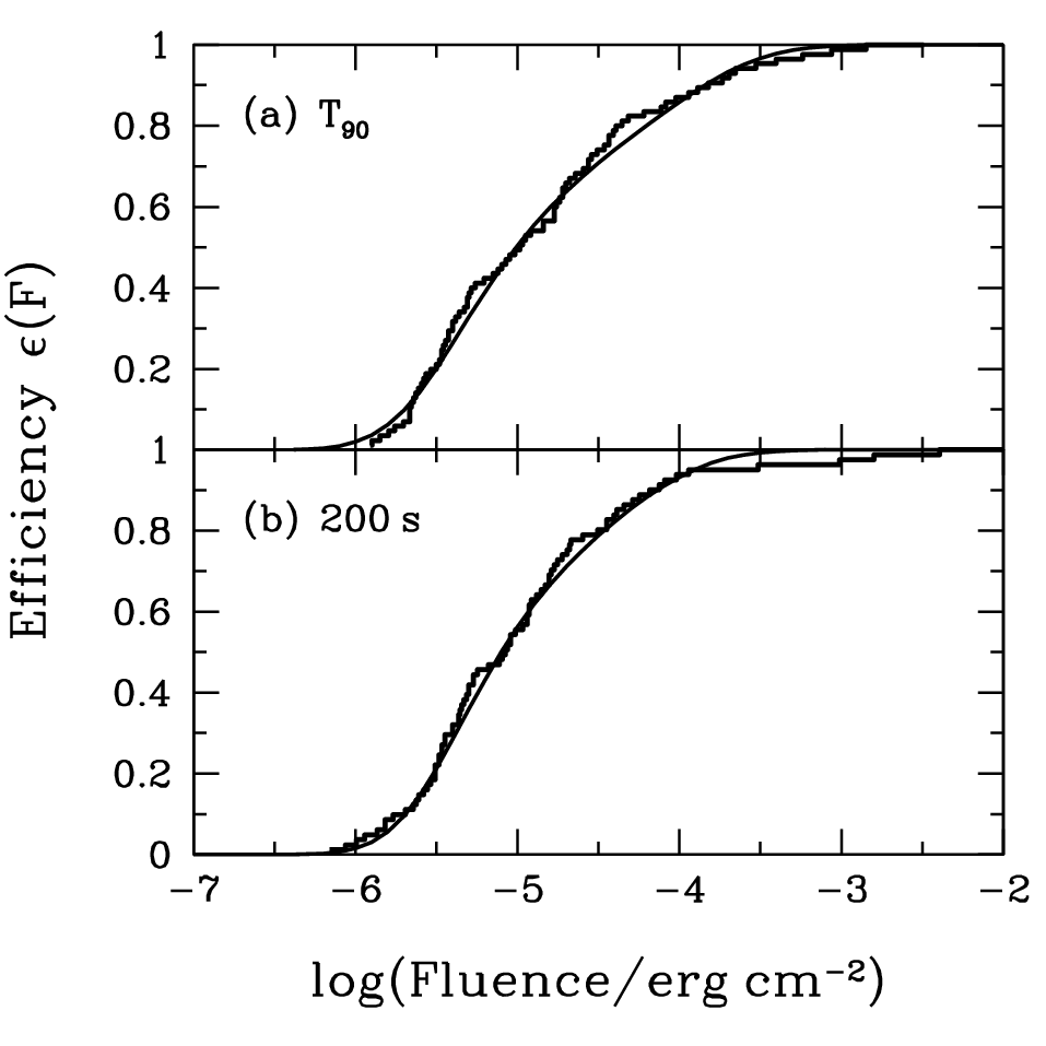
We used the observations to constrain and by carrying out a maximum likelihood analysis.33 3 The log likelihood of a distribution is calculated by integrating the probability between the error bars and below the upper limits of EGRET observations. For the fluence data, we used the results of Fig. 2.3 of González Sánchez [14] rather than Tables 2.1 and 2.2 there. Figure 2 shows the contour plot of the most likely region on the – plane for (top) and 200 s after data (bottom) assuming a spectral index of (if the spectral index is then increases by 1). In that procedure, detection efficiency of EGRET as a function of fluence, , is obtained from the distribution of the EGRET upper limits (for undetected GRBs), which is shown in Figure 3; i.e., a cumulative fraction of bursts whose fluence limits are below a given fluence. In the case of detected GRBs, on the other hand, the size of the error bars for the fluence is interpreted as measurement accuracy of EGRET. Then, in order to test the consistency of the assumption that equation (13) fits the data, we carried out a Monte Carlo simulation that draws realizations of EGRET observations assuming that the distribution of follows equation (13) with the most likely values of and . By comparing the likelihood of these Monte Carlo realizations with that of the actual EGRET observations, we find that 70% of the realizations have a lower likelihood, suggesting that equation (13) with its most likely values is indeed consistent with the observations.

Given and , we can obtain the distribution of fluence in EGRET band by convolving BATSE fluence distribution (; Fig. 1) and :
| (14) |
As representative models, we use three sets of for both the prompt and afterglow cases. These are labeled as AT90, BT90, and CT90 (A200, B200, and C200), and shown in Figure 2. In Figure 4, we show the resulting fluence distribution corresponding to each of these models.


EGRET results imply that during the prompt emission phase, . As we discussed in § II.1, the low number of photons in the bursts detected by EGRET, as well as their spectrum, implies that the detections of prompt photons are most likely to have been dominated by the high-energy tail of the synchrotron emission; i.e., in Figure 2(top). In fact, simply extrapolating synchrotron tail of many BATSE bursts up to 100 MeV regime, using inferred values for their and , gives a value of which is consistent with the one obtained here for the prompt phase. The harder IC prompt emission, however, can still have as much as 10 times larger fluence than that of the synchrotron emission in EGRET window, without being detected. Therefore, this figure also sets an upper limit on the ratio of the IC and synchrotron components of , as larger gives enough photon fluence detectable by EGRET. As we showed in § II.1, theoretically we predict (for EGRET) with a canonical set of parameters. Although this appears to imply that the current bound from EGRET already excludes the canonical model, we cannot make such a strong statement given the current uncertainties of many relevant parameters. Therefore, a more conservative statement would be that the current EGRET bound is barely consistent with the predictions of the SSC within the internal shock model. We may interpret the bound as constraints on and , which is shown in Figure 5(a). As the Klein-Nishina suppression () becomes significant for large , we have only modest limit on in such a regime. However, one should keep in mind that these are order of magnitude constraints, which may farther vary with other parameters, such as and . Much better constraint plot is expected with the future GLAST data, where hopefully, will be measured for many individual bursts.
During the afterglow the synchrotron emission is much softer than during the prompt phase, and therefore, the IC component is expected to dominate EGRET observations also near its lower energy-band limit. Moreover, the fact that the number of bursts detected by EGRET during the afterglow is higher than the number detected during the prompt emission suggests that here EGRET is likely to have detected the actual IC component of the afterglow. The spectral index of the GeV afterglow in EGRET window during the first 200 s is expected to be –2, implying that the evaluation of in the bottom panel of Figure 2, which assumes a spectral index of , might be larger by at most a small factor (2–3). Thus, for the afterglow, –. We then compare this result with the theoretical expectation of in equation (2). But first we need to estimate the value of where is measured during the first 200 s following and is the prompt emission fluence. We use the Swift GRB table44 4 http://swift.gsfc.nasa.gov/docs/swift/archive/grb_table/ which provides X-ray afterglow fluences several tens to several hundreds of seconds after the bursts, as well as the prompt MeV fluences. Using only bursts where the X-ray observation starts after but no more than s after the burst we find a distribution of that ranges from to , with the central value of 10-2. Thus afterglow theory with canonical parameters predicts with a large spread, consistent with EGRET constraints. Figure 5(b) shows the interpretation of EGRET constraint on (Fig. 2) as that for and , assuming canonical parameters and . Although this allowed region may change with other model parameters, again one cannot have too large value of because of the Klein-Nishina suppression factor .
IV. Implication for GLAST
| [s] | [erg cm-2] | [erg cm-2] | |
|---|---|---|---|
| 2.3 | 650 | ||
| 2.0 | 650 | ||
| 1.0aaHere we considered a detection based on the number of photons in the energy range 30 MeV–30 GeV. A higher and more sensitive background limited threshold can be obtained for if a higher energy range is considered (see text and Appendix B). | 650 |
Note. — Parameters of point-source fluence sensitivity (integrated over 30 MeV–30 GeV) of GLAST-LAT (see eq. [15]). The power-law index is , and the unit in fluence limit is erg cm-2. The detection criterion for is five photons, and significance for is , where s is the transition time.
We now move on to discussions on implications for GLAST using the obtained constraints on in the previous section. First we estimate the sensitivity of LAT on board GLAST for prompt and afterglow GeV emission, based on its published sensitivity to steady point sources,55 5 http://www-glast.slac.stanford.edu/ which is cm-2 s-1 above 100 MeV at with a power-law index of . This sensitivity is obtained by a one-year all-sky survey during which any point source is observed for 70 d (the LAT field of view is 2.4 sr).66 6 We assume here a step function for the LAT window function. Therefore during the background-limited regime (when is large enough that many background photons are observed) the flux limit scale with as cm-2 s-1 . During the photon-count-limited regime (when is so small that less than one background photon is expected), in contrast, the detection limit is at a constant fluence. Therefore the fluence sensitivity of the GLAST-LAT detector is
| (15) |
where s represents the time when the transition from photon-count-limited to background-limited regime occurs in the LAT case. Note that equation (15) is for the limiting fluence, the time-integrated flux, rather than the flux. This limit is more natural in the photon-count-limited regime and it is more relevant to EGRET constraints that we derived in the previous section. Detailed derivation of this sensitivity is given in Appendix B. In Table 1, we summarize the values of and for a few cases of power law index and integration time . The values of for in the table are determined by criteria of five-photon detection, while those for are by significance. The fluence we argue here is the one integrated over 30 MeV–30 GeV, in order to compare with the EGRET fluence upper bounds.
| Model | Rate at GLAST | [GeV cm-2 s-1 sr-1] |
|---|---|---|
| AT90 | 15 yr-1 | ) |
| BT90 | 20 yr-1 | ) |
| CT90 | 10 yr-1 | ) |
| A200 | 20 yr-1 | |
| B200 | 30 yr-1 | |
| C200 | 15 yr-1 |
Note. — The estimate of detection rate with GLAST-LAT (for ), and expected EGB intensity, for models A, B, and C of the prompt (during ) and afterglow phases (during 200 s after ). The correction factor for in the case of prompt emission could be as large as 10. Also note that these estimates are quite conservative. See discussions in §§ IV and V for more details.
In the case of background-limited regime, it might be more appropriate to use higher energy threshold (instead of 30 MeV) especially for hard source spectrum, because the background spectrum falls steeply with frequency (). We may find optimal low-frequency threshold depending on spectral index of GRB emissions; it is higher for harder spectrum. Thus, we should be able to improve the fluence sensitivity for background-limited regime, compared with the figures given in Table 1. In addition, transition from photon-count to background limited regime would occur later than 650 s. For our purpose, however, as time scales we consider ( for prompt emission and 200 s after for afterglows) are both during photon-count-limited regime, the consideration above does not apply and we can use full energy range (30 MeV–30 GeV for EGRET) to collect as many photons as possible.
GLAST is also equipped with the GLAST Burst Monitor (GBM) instrument, dedicated for the detection of GRBs. It detects photons of 8 keV to more than 25 MeV and its field of view is 8 sr. The expected rate of GRBs that trigger GBM is 200 yr-1 [25], which is almost as high as BATSE rate. Each year, about 70 out of these 200 bursts should fall within the LAT field of view. Given the distribution of fluences (Fig. 4) and the LAT sensitivity (Table 1), we can estimate the fraction of GRBs that would be detected with LAT. In Table 2, we show the expected LAT detection rate for , which is 20 yr-1 for the best-fit models of the EGRET data for both the prompt and afterglow emissions. The prompt phase estimates are for detections of the synchrotron component in the 100 MeV range. Given the large effective area of the LAT it is expected also to detect GeV photons from the IC component and identify the spectral break associated with the transition from the synchrotron to IC component, thereby directly testing the SSC model.
The estimates given in Table 2 are fairly conservative. First, while we used five-photon criterion for the detection, even two-photon detection should be quite significant, because the expected background count is much smaller than one photon during and the following 200 s that we considered. Second, Swift can find dimmer bursts than GBM. Although the discovery rate is not as high as that of GBM or BATSE, it would still be able to find tens of new GRBs in the LAT field of view. Thus the true rate would likely be larger than the figures given in Table 2.
V. Implication for the extragalactic gamma-ray background

All the GRBs except for those detected by EGRET should contribute to the EGB flux to a certain extent [11]. This may be computed as
| (16) |
where is EGRET fluence in 30 MeV–30 GeV, is the normalized distribution of EGRET fluence (eq. [14] and Fig. 4), and d-1 is the occurrence rate of GRBs from all sky. The factor takes into account the fact that very bright GRBs cannot contribute to the EGB because they would be identified as point sources (but see discussions below). Figure 6 shows differential EGB intensity that represents contribution from GRBs of a given fluence, for prompt and afterglow phases. In the third column of Table 2, we show the EGB intensity due to prompt and afterglow phases of GRBs which is 10-9 GeV cm-2 s-1 sr-1. On the other hand, in the same energy range, EGRET measured the EGB flux to be GeV cm-2 s-1 sr-1 [51]. Therefore, GRBs that were detected by BATSE but were not detected as point sources by EGRET contribute to the EGB at least 0.01%. Again, we note that the estimates for the prompt phase are those of synchrotron component. We thus need to take the predicted IC contribution into account, which is represented by a correction factor in Table 2. Since this factor could be as large as 10 according to the discussion in § III, EGB flux due to prompt phase of GRBs could also becomes 10 times larger, which makes GRB contribution as large as 0.1% of the observations above GeV. In any case, the contributions from other astrophysical sources such as blazars are expected to be more significant than GRBs [e.g, 2, and references therein].
Additional contribution to EGB is expected from a large number of GRBs that point away from us and therefore would not have been detected with BATSE. The emission from these bursts points towards us once the external shock decelerates [44]. Since the total GeV energy emitted every decade of time during the afterglow is roughly constant, the contribution of these GRBs to EGB can be estimated by the GeV emission of the bursts that were detected by BATSE. Similar contribution is expected from bursts that points towards us but that are too faint to be detected by BATSE, if the GRB luminosity function behaves as as suggested by the universal structured jet model [23, 45, 57, 39, see however Guetta, Piran, & Waxman 18]. Therefore the contribution of bursts that were not detected by BATSE to EGB can be estimated by the afterglow fluence of the detected bursts, assuming no contribution from bursts with only an upper limit. This is a reasonable estimate since the GeV flux is dominated by the few brightest bursts in GeV which are the most likely to be detected. Taking the fluence of the detected GeV bursts as the logarithmic mean of these upper and lower limits implies GeV cm-2 s-1 sr-1, a GRB contribution being 0.1% of the EGB.
Finally, we note that there is a big uncertainty in removing the Galactic foreground contamination from the total diffuse flux [22]. Additionally, EGRET observations do not constrain TeV emission that cascades down into the GeV range for GRBs at cosmological distances [6, 31]. Thus, if the foreground subtraction was indeed underestimated or if GRB TeV emission is not negligible, then GRB contribution might be much more significant than the estimates here.
VI. Summary and Conclusions
The GLAST satellite would enable us to test high-energy emission mechanisms of GRBs. If this emission will be found to be consistent with SSC then its observations would constrain physical parameters such as ratio and the bulk Lorentz factor of the jet, . The EGRET instrument on board CGRO, while less sensitive than the GLAST-LAT detector, identified several BATSE GRBs with GeV photons. In addition, stringent upper limits for 100 GRBs were put on fluences in the GeV band by analyzing the EGRET data [14].
In this paper, we further extended this EGRET result, comparing with the SSC emission model. Following theoretical models of SSC, we assumed that there is a linear correlation between fluences in BATSE and EGRET energy bands, and that the proportionality coefficient follows a log-normal distribution. We found that the predictions from the SSC model using canonical parameter values is fully consistent with EGRET fluence measurements and upper limits for both the prompt and afterglow phases. During the course of showing this result, we properly took the Klein-Nishina feedback effect into account in the theoretical calculation. The best-fit value of the coefficient was for both the prompt and afterglow emissions, and it is already stringent enough to test the SSC scenario. The limits for the prompt emission phase are for the synchrotron radiation, and thus if we consider the IC component as well, the value of could be larger by up to one order of magnitude.
The obtained distribution, together with the BATSE fluence distribution, gives the expected fluence distribution in the GeV band, which is shown in Figure 4. As the GLAST-LAT detector covers EGRET energy band, we can predict the detectable number of GRBs with GLAST from the distribution of , given the GLAST-LAT sensitivity. Our conservative estimate using the five-photon criterion is that about 20 GRBs among those detected with GBM would be detected with GLAST-LAT each year. This number could be even larger if we use fewer-photon criteria. The fluence distribution can also be used to estimate the GRB contribution to the EGB intensity. We found that the contribution would be at least 0.01% but is likely to be as large as 0.1%.
Appendix A Klein-Nishina feedback on high-energy emission
We shall find an analytic expression for due to the Klein-Nishina feedback. To simplify the argument such that we can treat it analytically, we make the following approximations: (i) an electron with a fixed Lorentz factor radiates mono-energetic synchrotron photons; (ii) the same electron upscatter a given synchrotron photon to another monochromatic energy, which is increased by a factor of ; (iii) of both synchrotron and IC photons peaks at (a synchrotron frequency corresponding to ) and ; if there is no Klein-Nishina suppression), respectively; (iv) the Klein-Nishina cutoff occurs quite sharply above its threshold; (v) both cooling and self-absorption frequencies are much smaller than the frequency region of our interest; and (vi) electrons cool so quickly that any dynamical effects can be neglected. With these approximations, expressions for the ratio of power of synchrotron and IC radiations from a given electron simplifies significantly. In particular, according to the assumption (iii) above, we have . This is given as
| (A1) |
where is electron spectral index, is the step function, and primed quantities are evaluated in the rest frame of the ejecta (e.g., , where is the frequency in an observer frame).
A detailed derivation as well as numerical approaches are given elsewhere (Nakar, Ando, & Sari, in preparation), but at least this equation can be understood qualitatively. For a given electron with Lorentz factor , the synchrotron power does not depend on whether the Klein-Nishina suppression is effective or not. On the other hand, the IC power does, because it is proportional to the energy density of seed (synchrotron) photons integrated up to some cutoff frequency; synchrotron photons above this frequency cannot be IC scattered efficiently by the electron with because of the Klein-Nishina suppression. The integrand of equation (A1) represents the synchrotron spectrum. More specifically, assuming there is no Klein-Nishina suppression, the spectrum is simply given by ; the step function then represents the Klein-Nishina cutoff. The factor in the denominator of the integrand accounts for the suppression of the electron distribution function due to the enhanced IC cooling; i.e., . These electrons are ones that emit synchrotron photons of a given frequency . Recalling the relation , their Lorentz factor is given by , which appears in the argument of in the integrand. Finally, the other constants in equation (A1) are chosen so that we have a proper relation for the fast cooling, , if we turn off the Klein-Nishina cutoff and have constant .
Now we shall find analytic expressions of equation (A1) in asymptotic regions. We start from the case of , which is equivalent to . The integration then becomes
| (A2) |
We assume that the function varies rather mildly in the integrand, so that in the argument of we may use . Then the integral can be evaluated analytically, and gives . When , we have , which is the same result as in the case of no Klein-Nishina suppression. This makes sense because the condition indicates that the electrons with is below the Klein-Nishina threshold with seed photons at frequency that dominate the synchrotron power. On the other hand, when (or ), equation (A1) becomes
| (A3) |
where in the second equality, we used for the argument of . When is large enough so that , then equation (A3) immediately gives asymptotic solution for . When is in the intermediate regime, we can still get analytic expressions, which however are given elsewhere because they are somewhat complicated. Here we simply show numerical solutions of equation (A1) as a function of for various values of . We show these results as well as a simple fitting form (given by eq. [5]) in Figure 7. Thus, equation (5) provides fairly good fit to the results of numerical integration of equation (A1).

Appendix B Fluence sensitivity of GLAST
For a steady point source with a spectral index of , the sensitivity of GLAST-LAT to its flux above 100 MeV is cm-2 s-1 at significance for a one-year all-sky survey. Considering the field of view of GLAST-LAT, 2.4 sr, this survey time corresponds to 70 d exposure time to the source, and therefore, the sensitivity to the number fluence integrated over this time scale is cm-2. In this section, we generalize this limit to an arbitrary spectral index, , and exposure time, .
Before starting the discussion, we define the differential number and energy fluences, and integrated number and energy fluences (all quantities are time-integrated):
| (B1) |
| (B2) |
where is a coefficient, and and are the energy band boundaries.
The fluence sensitivity for a one year exposure is within the background-limited regime—namely within one year many background photons are expected to be detected within the point-spread-function of the detector. In the case of GLAST-LAT, backgrounds are the EGB or Galactic foreground emissions. Therefore, we start our discussion from this background-limited case. Let us define this background rate of GLAST by , for which we assume spectrum and use the energy-dependent angular resolution and on-source effective area .77 7 For these specifications of the detector, we use the results shown in http://www-glast.stanford.edu/ The criterion of point-source detection is
| (B3) |
where represents significance of detection, and photon count from the source is obtained by
| (B4) |
Therefore, using equation (B1) in equations (B4) and (B3), we can obtain the sensitivity to the coefficient as follows:
| (B5) |
and then using equation (B2), this can be translated into the sensitivity to the number and energy fluences, and . We here note that depends on , , , and , while depends only on , , and . In this background-limited regime, the time dependence is from equation (B3). We confirmed that, using the EGB intensity measured by EGRET [51] and energy-dependent angular resolution of LAT, we could obtain the limit comparable to cm-2, in the case of , d, MeV, , and . The results of this procedure for several values of interest of are summarized in equation (15) and Table 1. Here, we used EGRET energy range, i.e., MeV and GeV, but we can instead adopt different values.
If the time scale is short such that , then the argument above does not apply, but the sensitivity is simply obtained by the expected photon count from the source. In this photon-count-limited regime, we can evaluate the fluence sensitivity by requiring to be a few; here we use . One can obtain the corresponding by solving this criterion using equation (B4). This time, is independent of . Then again using equation (B2), one can get the fluence sensitivity in this regime as shown in Table 1.
References
- [1] Ando, S. 2004, MNRAS, 354, 414
- [2] Ando, S., Komatsu, E., Narumoto, T., & Totani, T. 2007, Phys. Rev. D, 75, 063519
- [3] Asano, K., & Inoue, S. 2007, ApJ, 671, 645
- [4] Band, D., et al. 1993, ApJ, 413, 281
- [5] Baring, M. G., & Harding, A. K. 1997, ApJ, 491, 663
- [6] Casanova, S., Dingus, B. L., & Zhang, B. 2007, ApJ, 656, 306
- [7] Chiang, J., & Dermer C. D. 1999, ApJ, 512, 699
- [8] Derishev, E. V., Kocharovsky, V. V., Kocharovsky, V. V., & Mészáros, P. 2003, Gamma-Ray Burst and Afterglow Astronomy 2001: A Workshop Celebrating the First Year of the HETE Mission, 662, 292
- [9] Dermer, C. D., Chiang, J., & Mitman, K. E. 2000, ApJ, 537, 785
- [10] Dermer, C. D. 2006, preprint (astro-ph/0605402)
- [11] Dermer, C. D. 2007, American Institute of Physics Conference Series, 921, 122
- [12] Fan, Y.-Z., Piran, T., Narayan, R., & Wei, D.-M. 2008, MNRAS, 384, 1483
- [13] González, M. M., Dingus, B. L., Kaneko, Y., Preece, R. D., Dermer, C. D., & Briggs M. S. 2003, Nature, 424, 749
- [14] González Sánchez, M. M. 2005, Ph.D. Thesis
- [15] Gou, L.-J., & Mészáros, P. 2007, ApJ, 668, 392
- [16] Granot, J., Cohen-Tanugi, J., & Silva, E. d. C. 2007, preprint (arXiv:0708.4228 [astro-ph])
- [17] Guetta, D., & Granot, J. 2003, ApJ, 585, 885
- [18] Guetta, D., Piran, T., & Waxman E. 2005, ApJ, 619, 412
- [19] Hurley, K., et al. 1994, Nature, 372, 652
- [20] Ioka, K., Murase, K., Toma, K., Nagataki, S., & Nakamura, T. 2007, ApJ, 670, L77
- [21] Kaneko, Y., Preece, R. D., Briggs, M. S., Paciesas, W. S., Meegan, C. A., & Band, D. L. 2006, ApJS, 166, 298
- [22] Keshet, U., Waxman, E., & Loeb, A. 2004, J. Cosmology Astropart. Phys., 04, 006
- [23] Lipunov, V. M., Postnov, K. A., & Prokhorov, M. E. 2001, Astronomy Reports, 45, 236.
- [24] Lithwick, Y., & Sari, R. 2001, ApJ, 555, 540
- [25] McEnery, J., & Ritz, S. 2006, American Institute of Physics Conference Series, Vol. 836, Gamma-Ray Bursts in the Swift Era, pp. 660–663
- [26] Medvedev, M. V. 2000, ApJ, 540, 704
- [27] Mészáros, P., Rees, M. J., & Papathanassiou, H. 1994, ApJ, 432, 181
- [28] Mészáros, P. 2006, Rep. Prog. Phys., 69, 2259
- [29] Moderski, R., Sikora, M., Coppi, P. S., & Aharonian, F. 2005a, MNRAS, 363, 954
- [30] Moderski, R., Sikora, M., Coppi, P. S., & Aharonian, F. 2005b, MNRAS, 364, 1488
- [31] Murase, K., Asano, K., & Nagataki, S. 2007, ApJ, 671, 1886
- [32] Murase, K., & Ioka, K. 2008, ApJ, 676, 1123
- [33] Nakar, E. 2007, Phys. Rep., 442, 166
- [34] Panaitescu, A., & Kumar, P. 2000, ApJ, 543, 66
- [35] Panaitescu, A., & Kumar, P. 2001, ApJ, 560, L49
- [36] Panaitescu, A. 2008, MNRAS, 385, 1628
- [37] Pe’er, A., & Waxman, E. 2004, ApJ, 613, 448
- [38] Pe’er, A., & Waxman, E. 2005, ApJ, 633, 1018
- [39] Perna, R., Sari, R., & Frail, D. 2003, ApJ, 594, 379
- [40] Piran, T. 1999, Phys. Rep., 314, 575
- [41] Piran, T. 2005, Rev. Mod. Phys., 76, 1143
- [42] Preece, R. D., Briggs, M. S., Mallozzi, R. S., Pendleton, G. N., Paciesas, W. S., & Band, D. L. 2000, ApJS, 126, 19
- [43] Razzaque, S., Mészáros, P., & Zhang, B. 2004, ApJ, 613, 1072 fireballs and surroundings,”
- [44] Rhoads, J. E. 1997, ApJ, 487, L1
- [45] Rossi, E., Lazzati, D., & Rees, M. J. 2002, MNRAS, 332, 945.
- [46] Rybicki, G. B., & Lightman, A. P. 1979, Radiative Processes in Astrophysics. New York, Wiley-Interscience
- [47] Sari, R., & Esin, A. A. 2001, ApJ, 548, 787
- [48] Schneid, E. J., et al. 1992, A&A, 255, L13
- [49] Schneid, E. J., et al. 1995, ApJ, 453, 95
- [50] Sommer, M., et al. 1994, ApJ, 422, L63
- [51] Sreekumar, P., et al. 1998, ApJ, 494, 523
- [52] Strong, A. W., Moskalenko, I. V., & Reimer, O. 2004, ApJ, 613, 956
- [53] Waxman, E. 1997, ApJ, 485, L5
- [54] Wei, D. M., & Lu, T. 1998, ApJ, 505, 252
- [55] Yost, S. A., Harrison, F. A., Sari, R., & Frail, D. A. 2003, ApJ, 597, 459
- [56] Zhang, B., & Mészáros, P. 2001, ApJ, 559, 110
- [57] Zhang, B., & Mészáros, P. 2002, ApJ, 571, 876.