Variational calculation of the system based on chiral SU(3) dynamics
Abstract
The system, as a prototype for possible quasibound nuclei, is investigated using a variational approach. Several versions of energy dependent effective interactions derived from chiral SU(3) dynamics are employed as input, together with a realistic potential (Av18). Taking into account theoretical uncertainties in the extrapolations below the threshold, we find that the antikaonic dibaryon is not deeply bound. With the driving -wave interaction the resulting total binding energy is = 20 3 MeV and the mesonic decay width involving is expected to be in the range 40 - 70 MeV. Properties of this quasibound system (such as density distributions of nucleons and antikaon) are discussed. The , as an quasi-bound state of and a nucleon, appears to survive in the cluster. Estimates are given for the influence of -wave interactions and for the width from two-nucleon absorption processes. With inclusion of these effects and dispersive corrections from absorption, the binding energy is expected to be in the range 20 - 40 MeV, while the total decay width can reach 100 MeV but with large theoretical uncertainties.
pacs
Valid PACS appear hereI INTRODUCTION
In the context of low-energy QCD with quark flavors, the study of possible antikaon-nuclear quasibound states is a topic of great current interest. Spontaneously broken chiral symmetry, together with explicit symmetry breaking by the non-zero quark masses, basically determines the leading couplings between the low-mass pseudoscalar meson octet (Nambu-Goldstone bosons in the chiral limit) and the octet of the ground state baryons. In particular, the Tomozawa-Weinberg chiral low-energy theorem implies that the driving interaction in the isospin channel is strongly attractive. Likewise, the interaction is attractive. The coupling between these and channels is the prime feature governing the subthreshold extrapolation of the interaction. A detailed knowledge of this subthreshold interaction is required when exploring the possible existence of bound -nuclear clusters.
The quest for strong binding and dropping antikaon masses in a nuclear medium has a long history which originated in early discussions of kaon condensation in dense matter [1, 2] and continued over the years [3, 4, 5, 6] with increasing levels of refinement [7]. The topic has recently been revived when the existence of long-lived, deeply bound -nuclear states was suggested using a simple potential model [8]. It was argued that if the -nuclear binding is sufficiently strong to generate such systems below threshold, their width could indeed be small [8, 9]. Experiments performed in search for such states [10, 11, 12] have so far not given conclusive answers. While the search continues with more detailed analyses [13, 14, 15, 16, 17], “non-exotic” final state interaction scenarios cannot be ruled out as interpretation of the data [18].
An important prototype system for these considerations is , the simplest antikaon-nuclear cluster. It has recently been investigated using three-body (Faddeev) methods [19, 20] and variational approaches [21, 22, 23, 24]. Reaction studies [25] have also been performed dealing with the actual formation of . The Faddeev and variational calculations predict a total binding energy in a range 50 - 70 MeV, together with an estimate of the decay width, 50 - 100 MeV, depending on details of the interactions used.
The key issue in any such calculation is the (model dependent) extrapolation of the interaction into the region far below threshold. Its predictive power is so far limited by the persistent lack of accurate constraints from data. It is in this perspective that we perform the present variational calculation using a subthreshold effective interaction systematically derived from chiral SU(3) coupled-channel dynamics.
Apart from the constraints provided by threshold data and low-energy cross sections, the only piece of information about the interaction below threshold is the mass spectrum which is dominated by the resonance. The subthreshold extrapolation of the effective interaction has recently been investigated in detail [26] from the viewpoint of chiral SU(3) dynamics [27, 28, 29, 30, 31]. In this approach the off-shell amplitude below threshold is governed by the strong attraction in the and channels, and by the dynamical coupling of these channels. These couplings are again determined by the Tomozawa-Weinberg chiral low-energy theorem. Their structure shares features with the early pioneering coupled-channel model [32] that used vector meson exchange interactions (see also Ref. [33]).
Most chiral SU(3) based calculations agree that the resonance structure, with its nominal position at 1405 MeV as seen in the mass spectrum, is actually shifted to about 1420 MeV in the amplitude as a consequence of coupled-channel dynamics. This implies that the effective single-channel interaction is substantially weaker than anticipated in the simple phenomenological potential used previously in Refs. [8, 21]. In those phenomenological studies, the local, energy-independent potential was adjusted interpreting the directly as a bound state, identifying its binding energy by the location of the maximum observed in the spectrum, but ignoring strong coupled-channel effects.
In this paper we perform a variational calculation employing the new effective potential derived from chiral coupled-channel dynamics [26], together with a realistic potential.This calculation is supposed to be complementary to the Faddeev approach with chiral SU(3) constraints [20]. The variational calculation gives easy access to the wave function of the bound state so that valuable information about the structure of the cluster can be extracted, whereas the elimination of the channel is required and the width of the state can only be estimated perturbatively. The Faddeev calculation has, in turn, the advantage that the decay width of the quasibound state is computed consistently in the coupled-channel framework. Both methods therefore have their virtues and limitations which need to be discussed in comparison.
The present work extends and improves our previous studies [24] in several directions, including further refinements in the interaction, computation of density distributions, an evaluation of effects from -wave interactions and an estimate of the absorptive width. The paper is structured as follows. The variational framework and formalism are developed in Sec. II. The derivation of the effective interaction based on the chiral SU(3) coupled-channel approach is briefly summarized and discussed in Sec. III. Results of our calculations are presented in Sec. IV followed by a summary and conclusions in Sec. V.
II FORMALISM
II.1 Model wave function
In search for the energetically most favorable configuration, the present variational investigation focuses on the system with spin and parity and isospin , where the parity assignment includes the intrinsic parity of the antikaon. We prepare the following two-component variational trial wave function:
| (1) |
where is a normalization factor and is a mixing coefficient. The components and have the form
| (2) | |||||
| (3) | |||||
with spatial wave functions multiplied by the spin state vector of the two nucleons and the isospin state vector of the total system, respectively. In both components, the spin of the pair is assumed to be zero (). The large component has isospin () of the two nucleons corresponding to the dominant configuration, with inclusion of through charge exchange. The admixture of the component (), with zero isospin in the sector, can occur through a combination of and interactions and turns out to be small, typically less than 5%. Both components have the same total isospin .
The detailed ansatz for the spatial wave functions is chosen as follows:
| (4) | |||||
Here () and are trial functions describing the localization of the nucleons and the kaon, respectively. Their forms are assumed to be single Gaussians:
| (5) |
The and in Eq. (5) are treated as independent parameters. Correlations between the two nucleons, and between the and each nucleon, are described by corresponding correlation functions:
| (6) | |||||
| (7) |
The correlation function, , is prepared to account for the strong short-distance repulsion in the interaction which keeps the two nucleons apart. The correlation functions, , are given the flexibility to adjust themselves appropriately to the attractive antikaon-nucleon interaction.
One notes that the spatial wave functions , Eq. (4), are even or odd under exchange of the two nucleons:
| (8) |
The pair in () is thus in a singlet-even (singlet-odd) state. The spatial wave function is rotationally symmetric, i.e. the total orbital angular momentum is .
The trial wave function has the following real-valued variational parameters: in Eq.(1), and in Eq. (5), () in Eq. (6), and () in Eq. (7). The range parameters of the Gaussians in the and correlation functions are organized as
| (9) |
independently for each of the or sectors. Various combinations of parameter sets for the Gaussian ranges, , , (, ) and (, ) have been tried. For each combination of the range parameters, we find a set of parameters and which minimizes the expectation value of the total Hamiltonian, using the Simplex method [34]. This determines the bound state of minimal energy, if existent.
A remark should be added concerning the treatment of the center-of-mass (CM) motion. Given the independence of the variational parameters and in Eq. (5), the CM wave function cannot simply be separated by factorization in the present model. A complete separation is possible only in the special case , where () is the nucleon (kaon) mass. In the actual calculations we have confirmed that this relation between and turns out to be satisfied quite accurately even though it has not been imposed from the beginning. The variational procedure favors indeed a wave function in which the CM motion factorizes as it should. One typically finds fm-2 and fm-2, using the interaction based on chiral SU(3) dynamics and described in Sec. III.
II.2 Hamiltonian
The Hamiltonian used in the present study is of the form
| (10) |
Here is the total kinetic energy:
| (11) |
The energy of the center-of-mass motion,
| (12) |
is subtracted.
As a realistic nucleon-nucleon interaction we choose the Argonne v18 potential (Av18) [35]. Since the total spin of the two nucleons is restricted to zero as explained in the previous section, the tensor, and potentials do not contribute. We thus employ the central, and spin-spin parts of the Av18 potential:
| (13) |
where is a projection operator onto the singlet-even () or singlet-odd () state, and is the orbital angular momentum operator for the relative coordinate between two nucleons. The central and potentials [ and ] are identified with the phenomenological short- and intermediate-range parts of the Av18 potential, Eq. (20) in Ref. [35]. The long-range spin-spin term comes from one-pion-exchange, Eq. (17) in Ref. [35]. We ignore the electromagnetic part of Av18. Both and potentials are taken into account since our model wave function includes both types of states. In the present study the -dependence of each of the potential terms is well fitted by a series of Gaussians (see Appendix A). The most pronounced feature is the strong short-distance repulsion in the singlet-even central potential.
The energy-dependent effective -wave interaction is represented as
| (14) | ||||
| (15) |
where for each of the two nucleons, and , and is the isospin projection operator for the pair. In the present work, the radial dependence of the potential is assumed to be a single Gaussian form with range parameter . The interaction strength is a function of the (off-shell) center-of-mass energy variable of the system. This interaction, extrapolated into the subthreshold region, is a key issue in the present paper and will be specified in greater detail in a separate Sec. III.
II.3 Calculational procedure
The energy dependence of the interaction requires a self-consistent variational procedure to minimize the energy of the system. This is done in the same way as in our previous work [22].
We introduce an auxiliary (non-observable) antikaon “binding energy” to control the CM energy of the subsystem within the cluster. This is defined as
| (16) |
where is the nucleonic part of the Hamiltonian,
| (17) | |||||
| (18) |
The relation between the two-body energy and within the three-body system is not fixed. In general,
| (19) |
where is a parameter describing the balance of the antikaon energy between the two nucleons of the three-body system. One expects . The upper limit () corresponds to the case in which the antikaon field collectively surrounds the two nucleons, a situation encountered in the limit of static (infinitely heavy) nucleon sources. In the lower limit () the antikaon energy is split symmetrically half-and-half between the two nucleons. We investigate both cases and label them “Type I” and “Type II”, respectively:
| (20) | |||||
| (21) |
The calculations then proceed as follows. First, assume to be some trial starting value, . Given a relation between and , the strength of the potential is now fixed, and the Hamiltonian is determined. Then the variational calculation is performed to find the state of minimal energy. Given that state, a new antikaon binding energy, , is evaluated with the wave function so obtained. Then one examines whether coincides with . If not, a different starting value is chosen and the procedure is repeated until is satisfied at an acceptable level of accuracy.
The potential is in general complex. In order to perform the variational calculation of the energy and the “bound state” , the real part of the potential, , is used as a starting point. The decay width of that state is then calculated perturbatively by taking the expectation value of the imaginary part of the potential:
| (22) |
At this stage the width represents the mesonic two-body decay channels () within the three-body system. The non-mesonic absorption width for will be treated separately.
III EFFECTIVE INTERACTION
III.1 potential based on chiral SU(3) dynamics
Here we discuss the effective potential developed in Ref. [26]. This potential has been systematically constructed using chiral SU(3) coupled-channel calculations which successfully describe meson-baryon scattering and the properties of the dynamically generated resonance. The formulation of the coupled-channel approach is briefly sketched in Appendix B. Starting from this coupled-channel framework, a complex and energy-dependent interaction kernel is derived in the single channel, such that the full coupled-channel -wave scattering amplitude is exactly reproduced by solving the single-channel equation with . Then this effective interaction kernel is approximated by an equivalent local potential used in the Schrödinger equation (with reduced mass ),
| (23) |
The potential is expressed by the effective interaction kernel together with a normalized spatial distribution ,
| (24) |
where is the relative coordinate of the system and is the reduced energy of the two-body system.
An important observation in Ref. [26] and earlier work is that the diagonal coupling is strong enough to generate a resonance in the single (elastic) channel. In the strongly interacting system, the appears as a bound state embedded in the resonant continuum. The experimentally observed broad spectrum in the channel, with its maximum at 1405 MeV, is dominated by the inherent interaction, while the resonant structure in the amplitude, governed by the inherent interaction, actually appears around MeV. The “binding energy” commonly associated with the is therefore not 27 MeV but only less than half of this naive estimate. This small binding energy implies a weaker attractive potential, only about half as strong as the phenomenological potential of Refs. [8, 21]. One should nonetheless note that both phenomenological and chiral potentials reproduce the existing experimental data around threshold. Their qualitatively different subthreshold extrapolations result from the fact that the coupled-channels framework, constrained by the chiral effective Lagrangian, induces off-shell dynamics which is very different from the purely phenomenological approach.
Here we choose the spatial distribution of the potential as a Gaussian form
| (25) |
where is the range parameter. The strength of the approximate local potential is related to the interaction kernel defined in Ref. [26] as
| (26) |
The potential so obtained is complex and energy dependent, reflecting the elimination of the other (mainly ) channels. The center-of-mass energy is related to the binding energy of the two-body system as
We choose the range parameter such that the resonance structure is reproduced at the position predicted by the full chiral dynamics calculation. The scattering amplitudes for both and around threshold are also well reproduced by this potential.
However, the effective single-channel effective interaction is generally non-local. Naive translation of into an approximate local form does not guarantee that this local potential (we refer to it as “uncorrected”) reproduces the amplitude of the full coupled-channel calculation over a wide range of subthreshold energies. It is indeed found that simple extrapolation of the local potential (26) to the deep subthreshold region, MeV, significantly overestimates the scattering amplitude in comparison with that of the original coupled-channel approach [26]. Compensation of this deficiency requires modifying the strength of the real part of the potential and introducing extra energy dependence. The strengths of these “corrected” potentials in the and channels are parametrized by polynomials as
| (27) |
The coefficients are given in Ref. [26]. The strengths of the “corrected” and “uncorrected” potentials at are shown in Fig. 1, based on the chiral model of Ref. [37]. For the subsequent variational three-body calculation we always use the “corrected” potentials.

In order to estimate theoretical uncertainties we use altogether four different variants of chiral dynamics calculations from which we derive equivalent energy-dependent local potentials, ORB [36], HNJH [37], BNW [38], and BMN [39]. All these models reproduce the total cross sections for elastic and inelastic scattering, threshold branching ratios, and the mass spectrum associated with the . Differences among those models mainly stem from the lack of accurate data for the spectrum and from differences in details of the fitting procedures. The values of the range parameters for these models are shown in the second row in Table 1. Additional uncertainties, concerning higher order terms in the interaction kernel derived from chiral SU(3) dynamics, are estimated to be about 20 % around MeV, based on the systematic study of such higher order corrections in Ref. [38].
III.2 Structure of the
| ORB [36] | HNJH [37] | BNW [38] | BMN [39] | |
|---|---|---|---|---|
| [fm] | 0.52 | 0.47 | 0.51 | 0.41 |
| [MeV] | ||||
| [fm] | ||||
| [MeV] | ||||
| [MeV] |
Let us now examine the two-body system with where the is generated dynamically below the threshold. In order to study the structure of the , we first solve the Schrödinger equation (23) with the real part of the potential, . This treatment appears to be justified by the relatively small imaginary part of the potential as seen in Fig. 1. Corrections from the dispersive shift of the binding energy induced by the imaginary part of the potential will be estimated as we move along.
The self-consistent results for the binding energies are summarized in Table 1 together with the root mean distance () between antikaon and nucleon which form the . These results are produced with the “corrected” potentials, but the “uncorrected” ones give essentially the same output since the difference in strength between the “corrected” and “uncorrected” potentials is small in the energy region relevant to the bound state ( MeV). The typical binding energy and root mean distance found with the chiral potential,
| (28) |
should be compared with the results of the phenomenological model [21]: MeV and fm. The small binding obtained with the present potential is related to the strong interaction in chiral dynamics, as discussed in Ref. [26]. Since the binding energy is smaller, the size of the bound state becomes correspondingly larger than that of the phenomenological model.
It is instructive to recall the study of electromagnetic properties of the in chiral dynamics [40], where a relatively large electric mean squared radius has been reported. Although the electric mean squared radius is not directly comparable to the mean distance of antikaon and nucleon, qualitative agreement of these independent size estimates gives support to the chiral effective potential introduced here, while the radius in Ref. [40] was computed with the full chiral coupled-channel amplitudes.
III.3 Dispersive effects induced by the imaginary part of the potential
The variational calculation of the three-body problem has the disadvantage (unlike the Faddeev approach) that only the real part of the complex potential can be handled as input whereas the imaginary part must be treated perturbatively. It is therefore mandatory to estimate the systematic uncertainties caused by this limitation.
In the two-body case, the scattering amplitude can easily be obtained by solving Eq. (23) with the full complex potential. Effects of the dispersive shift on the binding energy, induced by the imaginary part of this potential, can then be examined by comparing the full result (with complex potential) to the one obtained using only the real part of the potential, see Eq.(28). The energy, , of the subthreshold state generated by the complex potential can be deduced from the zero of the real part of the scattering amplitude. For comparison we also check the position of the maximum, , of the imaginary part of that amplitude, which coincides with if the non-resonant background is small.
The calculated values of (and ) are listed, for all models considered, in Table 1. Comparing with the binding energies found with the real parts of the potentials, we conclude that the dispersive effects may increase the binding energy of the two-body quasibound state by
| (29) |
or - 10 MeV when comparing and . We keep this shift in mind for a discussion of systematic uncertainties when we now turn to the three-body system.
IV RESULTS
This section presents the results of our variational calculations of the quasibound system. Four variants of effective interactions have been employed: ORB, HNJH, BNW and BMN as explained in the previous section. These interactions are translated into local, energy-dependent potentials. In all cases we have used the “corrected” versions of the potentials which properly reproduce the scattering amplitude computed with full chiral coupled-channel dynamics. In the self-consistent treatment of the energy dependence of the interaction, both options, “Type I” [Eq. (20)] and “Type II” [Eq. (21)] for the relationship between and have been tried. With these different choices for on-shell equivalent potentials and different options for handling off-shell energies within the three-body system, we are in a position to give rough estimates of the uncertainties associated with the required subthreshold extrapolations. In all calculations, the convergence of the Gaussian expansions (6) and (7) has been checked and found satisfactory with .
IV.1 Total binding energy and decay width
| ORB | HNJH | BNW | BMN | |
|---|---|---|---|---|
| “Type I” | ||||
| [MeV] | 18.9 | 16.9 | 18.1 | 16.6 |
| [MeV] | 53.1 | 47.0 | 60.4 | 38.8 |
| “Type II” | ||||
| [MeV] | 22.7 | 20.8 | 20.7 | 21.7 |
| [MeV] | 64.2 | 58.3 | 71.4 | 53.1 |
The results of self-consistent solutions for total binding energies are summarized together with the decay widths in Table 2 and depicted in Fig. 2. In all present calculations the binding energies turn out to be quite modest. Deeply bound, narrow states are not seen to develop. The variational calculations, with as previously specified and treated according to Eq.(22), predicts total binding energies and decay widths in the range
for all cases studied. The “Type II” ansatz favors slightly stronger binding (20 - 23 MeV) than the “Type I” option (16 - 19 MeV). Different potentials produce binding energy variations within only about two MeV for each given “Type I” or “Type II” set.

It is instructive to examine the detailed decomposition of the total energy into kinetic and potential energies of the antikaon and two-nucleon subcomponents. These sets of numbers are given in Tables 3 and 4 for the four variants of chiral SU(3) based models mentioned previously. Shown (separately for the “Type I” and “Type II” options) are the total kinetic energy, , the nuclear part of the kinetic energy, , the antikaon binding energy defined in Eq. (16), the expectation value of the -nuclear potential energy, , and the contribution from the nucleon-nucleon interaction, .
Several interesting observations can be made. First, the kaon “binding energy” is in the range 40 - 50 MeV for all cases studied. Note, however, once again that is not an observable in the three-body system. In fact the observable total binding energy is less than half of . The nucleons are the slow movers in the quasibound compound: their kinetic energies add up to only about 40 MeV, while the total kinetic energy in the three-body cluster is typically more than three times larger and thus carried predominantly by the antikaon floating between the two slowly moving, heavy nucleons. The antikaon’s potential energy roughly cancels the total kinetic energy, leaving room for the nucleon-nucleon interaction to bind the system which, as an isolated proton-proton pair, would be unbound.
The admixture of the isospin-zero () component [Eq. (3)] is typically about 4%. It originates from the coupling matrix element which is proportional to the difference of and interactions. Although small, this admixture helps binding the system: without the component, the total binding energy would decrease by about 5 - 7 MeV as seen from the lines denoted “HNJH†” in Tables 3 and 4.
The spin-spin and parts of the potential have an influence on the admixture. The contribution of these terms to is small and attractive. It tends to reduce the mixing of the component into the total wave function. This is seen in the last lines of Tables 3 and 4 denoted by “HNJH∗” where the spin-spin and potentials are turned off and only the central part of the potential is active. The spin-spin and terms were not considered in our previous Ref. [24].
| ORB | 18.9 | 53.1 | 125.9 | 38.3 | 40.2 | 127.7 | 17.0 |
|---|---|---|---|---|---|---|---|
| HNJH | 16.9 | 47.0 | 129.5 | 38.1 | 38.9 | 130.4 | 16.2 |
| BNW | 18.1 | 60.4 | 124.9 | 37.4 | 39.2 | 126.7 | 16.3 |
| BMN | 16.6 | 38.8 | 141.5 | 39.9 | 40.8 | 142.5 | 15.7 |
| HNJH† | 12.0 | 44.8 | 115.1 | 37.0 | 31.0 | 109.0 | 18.2 |
| HNJH∗ | 15.9 | 47.1 | 129.6 | 37.3 | 38.9 | 131.2 | 14.3 |
| ORB | 3.4 % | 2.15 | 1.93 | 1.79 | 2.28 |
|---|---|---|---|---|---|
| HNJH | 3.8 % | 2.21 | 1.97 | 1.82 | 2.33 |
| BNW | 4.1 % | 2.20 | 1.97 | 1.81 | 2.35 |
| BMN | 3.8 % | 2.23 | 2.00 | 1.86 | 2.34 |
| HNJH† | 0 % | 2.13 | 2.01 | 2.01 | 2.01 |
| HNJH∗ | 4.5 % | 2.26 | 2.00 | 1.83 | 2.39 |
| ORB | 22.7 | 64.2 | 136.0 | 40.9 | 46.1 | 141.2 | 17.6 |
|---|---|---|---|---|---|---|---|
| HNJH | 20.8 | 58.3 | 141.0 | 40.9 | 45.1 | 145.2 | 16.6 |
| BNW | 18.1 | 71.4 | 132.0 | 39.3 | 43.2 | 136.0 | 16.7 |
| BMN | 21.7 | 53.1 | 158.4 | 43.8 | 49.3 | 163.9 | 16.2 |
| HNJH† | 13.8 | 51.8 | 121.3 | 38.7 | 33.9 | 116.5 | 18.5 |
| HNJH∗ | 19.8 | 58.6 | 141.5 | 40.3 | 45.2 | 146.4 | 14.9 |
| ORB | 3.7 % | 2.10 | 1.85 | 1.71 | 2.21 |
|---|---|---|---|---|---|
| HNJH | 4.1 % | 2.15 | 1.89 | 1.73 | 2.26 |
| BNW | 4.1 % | 2.16 | 1.91 | 1.75 | 2.29 |
| BMN | 4.1 % | 2.15 | 1.89 | 1.73 | 2.25 |
| HNJH† | 0 % | 2.09 | 1.96 | 1.96 | 1.96 |
| HNJH∗ | 4.8 % | 2.19 | 1.91 | 1.74 | 2.31 |
IV.2 Structure of the cluster
Consider now the more detailed structure and characteristic sizes of the system as found in the present calculations. For this purpose we introduce density distributions of the and pairs in the quasibound compound as functions of the respective nucleon-nucleon and antikaon-nucleon distances, as follows:
| (30) | |||||
| (31) |
where refer to the two nucleons and to the antikaon. Both densities are understood as being normalized to one. The projected density distributions for pairs with specific isospin are
| (32) |
with the isospin projectors .
With these distributions one can determine mean-square distances
| (33) | |||||
| (34) | |||||
| (35) |
with . These average distances are summarized in the lower parts of Tables 3 and 4. The relatively weak binding of the system implies rather large distances, typically around fm, while the average distances are slightly smaller, fm. When looked at separately in the and channels of the subsystem, the significantly stronger attraction in the component drags the antikaon closer to the nucleon than in the component.
The different density distributions, Eqs. (30-32), are shown in Figs. 3 and 4. These densities depend only on the absolute value of the relative coordinate . The two-body densities are plotted as functions of and normalized as . The two-nucleon distribution shows the pronounced effect of the short-distance repulsive core of the interaction. The maximum density reached in this weakly bound system is about 0.03 fm-3, a small fraction of typical bulk nuclear densities and only twice as large as the maximum proton-neutron density in the even more dilute, very weakly bound deuteron.
The density distribution has its maximum at zero distance between the antikaon and each nucleon. It reflects the strong attraction in the channel, whereas the density is small. The right panel in Fig. 4 shows a comparison between densities of the pair in the cluster and the one forming the as a two-body quasibound state. Both densities are properly normalized for the comparison. The conclusion to be drawn from this picture is that the stays essentially intact in the system which appears to behave much like a weakly bound, short-lived compound. Again, the component of the total density is small. A detailed analysis of the expectation values of the squared angular momentum, in the system shows that it is close to zero in and close to two in configurations, indicating as expected the dominant -wave in the channel. The survival of the in the three-body cluster is qualitatively consistent with the result of the phenomenological potential [21].


IV.3 Comparison with Faddeev results
The small binding energy of only about 20 MeV found in the present variational approach appears to be inconsistent with results of a Faddeev calculation using a chiral interaction [20] which predicts about 80 MeV binding. Here we discuss possible reasons for this difference.
An advantage of the Faddeev treatment is its capability to treat the three-body dynamics in the channel. The variational approach, on the other hand, works with an effective interaction after eliminating the channel. While the attractive two-body interactions and their coupled-channel effects are nonetheless accounted for as part of the complex and energy dependent potential, additional attraction may indeed be generated by the three-body dynamics treated explicitly in the Faddeev approach.
Secondly, there are significant differences in the subthreshold extrapolations of the two-body interaction. When solving Faddeev equations, a one-term separable form has been used to approximate the interaction [20]. While this interaction agrees with ours in its on-shell properties around threshold, it has been pointed out in Ref. [26] that using such a separable approximation gives stronger attraction at lower (subthreshold) energies, as an artifact of the regularization procedure. This is also evident by comparison of subthreshold extrapolations with early works on chiral SU(3) coupled-channel dynamics which had adopted separable forms for the and interactions [27]. In contrast, the potential in the present investigation is constructed using dimensional regularization of loops in the Bethe-Salpeter equation11 1 This is equivalent to a dispersion relation approach, absorbing uncontrolled high-energy behavior in a few subtraction constants. (see Appendix B for a further detailed assessment of different regularization schemes). The resulting subthreshold amplitudes have significantly smaller real parts in comparison with those using the separable approximation. The reason for this behavior can be traced to the three-momentum form factors commonly used in separable interactions. Standard analytic continuation of the momentum variable into the subthreshold region lets these form factors increase beyond their threshold (zero-momentum) magnitudes, thereby enhancing the subthreshold amplitude artificially. While such analytic continuations need not be performed in the Faddeev approach, this example nevertheless demonstrates that extrapolations into the far-subthreshold region are confronted with off-shell uncertainties which severely restrict the predictive power of binding energy calculations.
Next, we examine the dispersive effect induced by the imaginary part of the potential. The advantage of the Faddeev method is its ability to deal consistently to all orders with the imaginary parts of the interactions whereas the variational method can handle this only perturbatively. In Section III.3 we have estimated that dispersive corrections from these imaginary parts amount to about MeV binding per nucleon, based on the analysis of the two-body channel. Thus the dispersive correction to the system would add another MeV to the total binding energy.
On top of these effects, there are several minor differences between two schemes such as the potential, admixture of the component, and so on. These factors might work together to contribute to the difference between the present result and that in Ref. [20].
We add a short comment on the sensitivity of the results to details of the potentials. In fact, as long as the system is only weakly bound, the dependence on different types of interactions is weak. We have performed test calculations using a soft-core potential quite different from Av18 but equivalent with respect to reproducing low-energy data. The resulting properties of the quasibound system turn out to be very similar to those obtained with the Av18 interaction. Details are given in Appendix D.
IV.4 Corrections from -wave interactions
A rough leading-order estimate of the effect of -wave interactions can be performed by computing expectation values of suitably parametrized -wave and potentials. The -wave effective potentials used here,
| (36) |
with and the reduced energy , involve the energy-dependent -wave scattering “volumes” for -proton and for -neutron, where . Their prominent feature is the resonance. We use a parametrization updated from Ref. [41] which has also been used in our previous study [22]. The energy dependence of is shown in Fig. 5.

Expectation values of this -wave potential are then computed with the wave functions of all four chiral models under consideration, changing the range parameter within a reasonable interval, 0.4 fm to 0.9 fm. Then is found to be small and repulsive,
| (37) |
The weak binding of the system places the effective for the subsystem above the position of the , hence the positive sign of . The contribution of -wave interactions is small if the binding from the driving -wave interactions is relatively weak as it turns out in the present work. If the binding were strong enough to move the effective energy of the pair down below the resonance, the -wave potential would act attractively and would tend to increase the binding. The present results appear to rule out this possibility.
For the correction to the width from -wave interactions one finds - 35 MeV. This relatively large (especially for the type I case) results from the fact that the two-body energy of the subsystem is located close to the resonance with its prominent imaginary part, see Fig. 5. Obviously we can give here only a rough estimate for orientation.
IV.5 Estimate of antikaon absorption by the two-nucleon pair
A further point of interest is the contribution to the decay width of the cluster from the two-body absorption process . This effect is not included in the imaginary part of the potential used to estimate the decay width (22) in previous sections.
For first guidance, let us start with the formula of the decay width for absorption on proton pairs in a heavy nucleus [42, 43, 44]
| (38) |
where and are the one-body densities of nucleon and antikaon, is the energy of the meson, and is a kinematical factor normalized to unity at threshold, [42, 44]. This factor reflects the phase space and kinematics for the relevant decay channels (, , and in the present case):
where and , . Eq. (38) derives from an effective contact interaction, with the coupling strength estimated empirically as fm4 [44] on the basis of kaonic atom data summarized and discussed in Refs. [42, 43].
The absorptive width in the form (38) is proportional to the probability of finding three particles (antikaon and two nucleons) at the same space point, as expressed by the product of the one-body densities. This treatment is justified for large nuclei where the independent particle picture works reasonably well. However, for the few-body system, the following modifications are required:
- (i)
correlations between the two nucleons must be taken into account, and
- (ii)
finite range effects in the absorption process must be considered.
The first modification is mandatory because of the repulsive core in the nucleon-nucleon interaction. Once the correlations are taken into account, a local absorptive contact interaction (38) is not appropriate because it provides almost no width: the probability for two nucleons to be found at the same spot is basically zero. A proper treatment must therefore deal with finite range effects in the absorption process which in turn requires a more detailed assessment of the underlying microscopic mechanisms.
By analogy with pion absorption in the deuteron, a leading microscopic process would be one-pion exchange (Fig. 6, left). This process, however, does not contribute to absorption on a proton-proton pair with spin in the system considered here. So the driving absorption mechanism is expected to come from exchanges of two pseudoscalar mesons as illustrated in Fig. 6. In chiral effective field theory, these are subleading one-loop terms in the two-baryon system involving or couplings to one of the baryons and exchange of the (interacting) two mesons with the second baryon. These processes occur when the external antikaon overlaps with one of the nucleons. The effective range of the absorption process is then related to the mass spectrum representing the exchanged two-meson system.

Thus, in order to estimate the width from the two-nucleon absorption process, we need to extend the formula (38) to satisfy the requirements (i) and (ii). The result should reduce to the original form (38) in the limit of no correlations and zero-range interaction, so that contacts to phenomenology can be made concerning the absorptive coupling strength .
First note that the product of one-body densities can be expressed as
| (39) |
For the modification requested by item (i), we introduce the three-body density as
where the function represents the correlations among the particles. The product of one-body densities in Eq. (39) can now be replaced by the three-body density which reduces to the original form in the limit of . The modification (ii) is implemented by replacing the delta function in Eq. (39) by a finite range distribution, such as a normalized Gaussian:
Taking , this distribution turns into the delta function. In summary, the formula for the absorptive width of the few-body system is given by
| (40) |
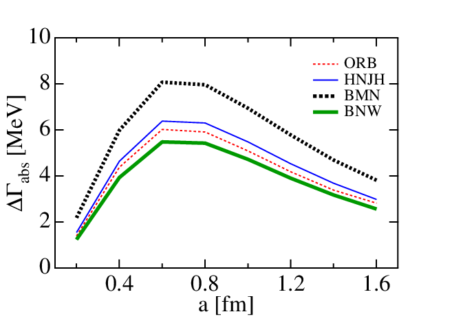
The variation of with respect to changes of the Gaussian range parameter is shown in Fig. 7. Note that, from the point of view of the microscopic or exchange mechanisms discussed previously, the characteristic ranges are covering a band from fm for exchange to about fm for uncorrelated exchange. For a typical choice of the absorptive coupling strength, fm4 and fm, one finds:
| (41) |
for all models (with Type I or Type II ansatz). The coupling strength is, of course, subject to considerable uncertainties. From the recent survey [43] based on kaonic atom data analysis one estimates a possible band width fm4 [44] which translates into
| (42) |
Given this estimated upper limit for in the system we conclude that the absorptive width in such a dilute, weakly bound system is expected to be less important than the one from the mesonic decay under the given conditions. This situation may change qualitatively for heavier nuclei with potentially stronger binding where the absorptive width can be far more prominent as pointed out in Ref. [44].
V SUMMARY
We have investigated the prototype of antikaonic nuclei, , using a variational approach with an effective interaction derived from chiral SU(3) coupled-channel dynamics. Several versions of such interactions have been employed in the calculations. They all satisfy the necessary constraint of reproducing empirical threshold information and the mass spectrum in the region of the , within (admittedly large) uncertainties of the existing experimental data base. Furthermore, a realistic nucleon-nucleon interaction (Argonne v18) has been used throughout. This interaction properly accounts for repulsive short-distance correlations.
The primary problem faced in the theoretical part of the quest for antikaon-nuclear quasibound systems is the subthreshold extrapolation of the -wave interaction. As a consequence of the strong coupled-channel dynamics, this interaction is complex, non-local and energy dependent. While the driving interaction kernel is determined by chiral SU(3) dynamics, the off-shell extrapolation into the far-subthreshold region is subject to uncertainties which limit the predictive power of the theory. A minimal condition for any such calculation is to account in detail for the coupled-channel dynamics that governs the formation of the as a quasibound state embedded in the strongly interacting, resonant continuum. When this is done, the resulting effective potential turns out to be significantly less attractive than anticipated in a simple phenomenological approach using a local, energy-independent potential. As a consequence we arrive at weaker binding than that previously suggested.
As an independent test of the variational method applied in the present investigation, we have performed calculations using the phenomenological Akaishi-Yamazaki (AY) potential. The stronger binding found with this energy independent local potential is indeed reproduced as reported in detail in Appendix C.
The results of the present variational calculation are summarized as follows:
- •
The calculated binding energy of the cluster, based on the leading -wave interaction only, is
where the error indicates variations using four different versions of chiral SU(3) coupled-channel calculations. The decay width into final states is estimated to be in the range
- •
Differences between these variational results and those obtained from Faddeev calculations [20] presumably relate in large part to three-body dynamics not incorporated in the present framework. Some part of these differences may be attributed to the use of separable approximations for the and interactions when solving Faddeev equations, and to dispersive effects not covered by the variational approach. We estimate the dispersive correction to the total binding energy to be MeV.
- •
This additional binding is partly compensated by corrections from -wave interactions which have a repulsive effect as long as the effective two-body energy in the subsystem stays above the resonance. The overall binding energy, after corrections and with conservative error assignment, is then expected to be in the interval - 40 MeV.
- •
The -wave interactions tend to increase the mesonic decay width for by an amount of 10 - 35 MeV.
- •
The additional effects of absorption are estimated to increase the decay width of the quasibound state further by an mount of order 10 MeV.
- •
In the variational approach the wave function of the quasibound state can be computed and analyzed. Given its weak binding, the system is rather dilute. The average distance between the two nucleons is about fm. The short-range repulsion in the interaction plays an important role in keeping the nucleons apart. The antikaon likes to minimize its distance from either nucleon. The isospin density distribution within the cluster is reminiscent of the in the two-body system, indicating a dibaryonic hybrid structure. However, with its estimated lifetime of order fm/c, this structure can exist only over a very short time interval.
Taking all theoretical uncertainties into account, we arrive at the conclusion that narrow, deeply bound clusters are unlikely to exist. Our calculation predicts such systems to be weakly bound and short-lived. With a rather low binding energy and a total width between 60 and 120 MeV, such structures would indeed be difficult to detect. One should keep in mind, however, that the present calculations rely entirely on the constraints provided by the presently available sets of threshold data and the poorly known mass spectrum. Improvements of this data base will sharpen the theoretical input conditions for deriving the effective subthreshold interaction. One can look forward to further developments along these lines as the experimental searches proceed with higher precision.
ACKNOWLEDGEMENTS
We thank Avraham Gal for fruitful and stimulating discussions. One of authors (A. D.) is grateful to Prof. Akaishi for advice on the construction of our model wave function. This project is partially supported by BMBF, GSI and by the DFG excellence cluster “Origin and Structure of the Universe”. T. H. thanks the Japan Society for the Promotion of Science (JSPS) for financial support. This work is also supported in part by the Grant for Scientific Research (No. 19853500, 19740163) from the Ministry of Education, Culture, Sports, Science and Technology (MEXT) of Japan. This research is part of Yukawa International Program for Quark-Hadron Sciences.
Appendix A NN potentials


| 1 | 2 | 3 | 4 | |
|---|---|---|---|---|
| 3708 | 483 | 44 | 3 | |
| 0.411 | 0.726 | 1.317 | 2.619 | |
| 651 | 412 | 43 | 6 | |
| 0.453 | 0.603 | 1.092 | 2.622 | |
| 47 | 57 | 5 | ||
| 0.383 | 0.637 | 1.009 | ||
| 170 | 27 | 0.3 | ||
| 0.537 | 0.804 | 1.644 |
For practical convenience in performing the variational calculations, the original Av18 potential has been represented by a series of Gaussians.
The spin state of the two nucleons is restricted to in our model, so the expectation value of the operator in the spin-spin potential is equal to . We have fitted the radial parts of the central potential plus the spin-spin potential, , with four Gaussians of different ranges; the radial part of potential, , is fitted with three Gaussians:
| (43) | |||||
| (44) |
with strengths and and ranges and , where indicates the channels , . The values of the parameters are listed in Table 5. For illustration of the fit quality we draw the potentials in Figs. 8 and 9.
Appendix B Chiral coupled-channel approach and regularization dependence
Here we briefly summarize basics of the chiral SU(3) coupled-channel approach [26]. In particular, we study the regularization dependence of the and amplitudes, an issue that has repeatedly been raised in the literature.
The starting point is the coupled-channel meson-baryon scattering equation
| (45) |
with the interaction kernel derived from the chiral SU(3) meson-baryon Lagrangian, and the loop function to be discussed in detail later. In order to derive the single-channel potential, an effective interaction kernel is constructed such that the full solution of Eq. (45) in the channel is reproduced by solving a single-channel scattering equation with :
| (46) |
where now represents the channel. This is used in Eq. (26) to determine the strength of the potential.
In Ref. [26], dimensional regularization was used in the calculation of the loop function . Dimensional regularization has the advantage that the analyticity of the loop function is compatible with the dispersion relation used in the N/D method [29]. It is however instructive to study the regularization dependence in this framework, in order to understand possible differences between present results for the system and the results of the Faddeev calculation with interactions constrained by chiral dynamics [20]. An analysis of the regularization dependence in this framework can be found in Ref. [45]. Note that differences in the regularization schemes only change the loop function and leave the interaction kernel untouched.
Using dimensional regularization, the loop function is given by
| (47) |
where are subtraction constants, is the renormalization scale, and we have defined
With a sharp three-momentum cutoff, the loop function is
| (48) |
where is the three-momentum cutoff and
A smooth cutoff can be introduced using the Pauli-Villars method which corresponds to multiplying a monopole form factor
to the loop function, leading to
| (49) |
where
The real parts of the loop functions (47), (48), and (49) for and channels are plotted in Fig. 10. The imaginary parts are determined by the phase space of intermediate meson-baryon states and therefore independent of the regularization procedure. The parameters for the dimensional regularization and three momentum cutoff schemes are taken from phenomenologically successful models [28, 36]:
The loop functions and are evidently quite similar. Furthermore, choosing the parameter of the monopole form factor as
the corresponding loop functions behave quantitatively similar as those with dimensional/three-momentum cutoff schemes, as seen in Fig. 10. The cutoff scales of the form factors (several hundreds of MeV) is typical and naturally expected from meson-baryon phenomenology.
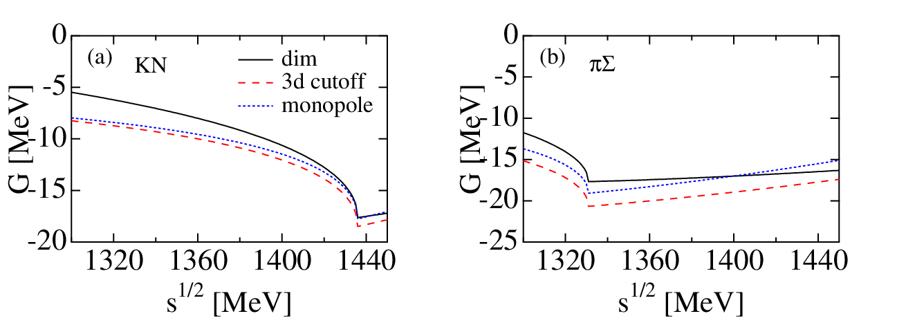
In summary, we find that smooth cutoff schemes provide similar loop functions as those with sharp cutoff or dimensional regularization. Since differences in the regularization schemes only affect the loop functions in the present framework, it is clear that the potentials derived in Ref. [26] remain unchanged when adopting a smooth cutoff.
In this respect, the difference between the present results for binding and those in Faddeev method [20] cannot be attributed to the regularization method. It is worth noting that early studies using the coupled-channel approach [27] gave a stronger subthreshold amplitude than the one derived in Ref. [26]. The calculations of Ref. [27] used a separable approximation for the potential together with the non-relativistic Lippmann-Schwinger equation, a feature also shared by the Faddeev calculations of Ref. [20]. Thus the larger binding energy of found in Ref. [20] is likely to be related to the type of scattering equation and the separable approximation used in that work.
Appendix C Benchmark test with the AY potential
As a test for the variational method and trial wave functions applied in the present work, we perform a calculation with the interaction [the Akaishi-Yamazaki (AY) potential] and the interaction (the Tamagaki potential) used in Ref.[21]. The AY potential is an energy-independent, local potential based on phenomenology but not constrained by chiral SU(3) dynamics.
The results are summarized in Table 6. The first two columns (“Model I” and “Model II”) show our results; the last column (“ATMS”) is the original result reported in Ref. [21]. In “Model I” the energy variation is performed restricting the wave function to its dominant component, i.e. with no admixture of the state (the one with coupled to isospin ), keeping the coefficient in Eq.(1). “Model II” includes the component, with determined variationally. In all calculations, the convergence of the Gaussian expansions (6) and (7) has been checked and found satisfactory with .
| Model I | Model II | ATMS | |
|---|---|---|---|
| 0 | finite | — | |
| 39.0 | 51.4 | 48 | |
| 60.0 | 61.0 | 61 | |
| 65.8 | 80.0 | 68 | |
| 46.7 | 47.8 | ||
| 147.0 | 162.4 | 167 | |
| 19.8 | 19.2 | 19 | |
| 166.2 | 194.6 | 196 | |
| 1.75 | 1.83 | 1.90 | |
| 1.54 | 1.55 | 1.57 | |
| 0 | 5.9 % | — |
One evidently finds a high degree of consistency between “Model II” and “ATMS”, confirming that the different variational methods used here and in Ref. [21] are of comparable quality.
The importance of the component of the wave function is underlined by the comparison between “Model I” with “Model II”. Although this admixture is only about 6 % as shown in the last row [] in Table 6, switching it off reduces the binding energy by more than 20 %. The matrix elements of the interaction taken between normalized states and are as follows:
| (50) | |||||
| (51) | |||||
| (52) |
The mixture implied by Eq. (52) increases the binding energy. For the AY potential the values of these three matrix elements are MeV, MeV and MeV, in this order. Taking the mixing ratio between and into account, the actual contributions from each matrix element to the potential energy are MeV, MeV and MeV, respectively, and so the coupling matrix element (52) is found to be attractive and non-negligible.
In concluding this Appendix we note again that the overall attraction produced by the based on chiral SU(3) dynamics, and used in the present work, is considerably weaker in comparison and leads to a binding energy less than half of that found with the simple AY potential.
Appendix D Dependence on the potential

Test calculations have been performed replacing the Av18 by a soft-core potential, the Minnesota potential [46] (see Fig. 11). This potential reproduces low-energy data (scattering lengths, effective ranges, and deuteron properties) just like the more realistic Av18 interaction. In the actual computations, we have fixed a parameter of the Minnesota potential () so that it corresponds to a Serber-type potential.
| HNJH | AY | |||
|---|---|---|---|---|
| Av18 | Minnesota | Av18 | Minnesota | |
| 16.9 | 17.0 | 49.0 | 50.4 | |
| 47.0 | 49.4 | 60.1 | 64.7 | |
| 38.9 | 42.1 | 78.1 | 84.2 | |
| 22.0 | 25.1 | 29.1 | 33.8 | |
| 38.1 | 32.9 | 49.5 | 41.3 | |
| 129.5 | 131.3 | 160.6 | 160.0 | |
| 16.2 | 7.8 | 20.5 | 7.5 | |
| 130.4 | 140.5 | 189.2 | 202.9 | |
| 2.21 | 2.15 | 1.82 | 1.80 | |
| 1.97 | 1.93 | 1.56 | 1.53 | |
| 3.8 % | 4.5 % | 4.4 % | 5.1 % |

Results of calculations are summarized in Table 7 for the chiral potential (HNJH) and for the phenomenological AY potential. The sensitivity to details of the interaction turns out to be marginal for the weakly bound system and slightly more pronounced but still weak for the more strongly bound AY case. The qualitative difference between strong and soft short-range repulsive core becomes apparent, however, when examining the density distribution within the clusters (see Fig. 12).
References
- [1] D. B. Kaplan and A. E. Nelson, Phys. Lett. B175, 57 (1986).
- [2] D. B. Kaplan and A. E. Nelson, Nucl. Phys. A479, 273 (1988).
- [3] G. E. Brown, C. H. Lee, M. Rho, and V. Thorsson Nucl. Phys. A567, 937 (1994).
- [4] T. Waas, N. Kaiser, and W. Weise, Phys. Lett. B379, 34 (1996).
- [5] T. Waas and W. Weise, Nucl. Phys. A625, 287 (1997).
- [6] T. Waas, M. Rho, and W. Weise, Nucl. Phys. A617, 449 (1997).
- [7] M. F. M. Lutz and C. L. Korpa Nucl. Phys. A700, 309 (2002); M. F. M. Lutz, C. L. Korpa and M. Moller, Nucl. Phys. A 808, 124 (2008).
- [8] Y. Akaishi and T. Yamazaki, Phys. Rev. C 65, 044005 (2002); T. Yamazaki and Y. Akaishi, Phys. Lett. B535, 70 (2002).
- [9] A. Dot, H. Horiuchi, Y. Akaishi and T. Yamazaki, Phys. Lett. B590, 51 (2004); Phys. Rev. C 70, 044313 (2004).
- [10] T. Suzuki et al., Phys. Lett. B597, 263 (2004).
- [11] T. Kishimoto et al., Prog. Theor. Phys. Suppl. 149, (2003) 264; Nucl. Phys. A754, 383 (2005).
- [12] M. Agnello et al., (FINUDA collaboration), Phys. Rev. Lett. 94, 212303 (2005).
- [13] T. Kishimoto et al., Prog. Theor. Phys. 118, 181 (2007).
- [14] M. Agnello et al., Nucl. Phys. A775, 35 (2006).
- [15] M. Sato et al., Phys. Lett. B659, 107 (2008).
- [16] T. Suzuki et al., Phys. Rev. C 76, 068202 (2007).
- [17] T. Suzuki et al., arXiv:0711.4943 [nucl-ex].
- [18] V. K. Magas, E. Oset, A. Ramos and H. Toki, Phys. Rev. C 74, 025206 (2006); V. K. Magas, E. Oset and A. Ramos, Phys. Rev. C 77, 065210 (2008).
- [19] N. V. Shevchenko, A. Gal, and J. Mares, Phys. Rev. Lett. 98, 082301 (2007); N. V. Shevchenko, A. Gal, J. Mares, and J. Révai, Phys. Rev. C 76, 044004 (2007).
- [20] Y. Ikeda and T. Sato, Phys. Rev. C 76, 035203 (2007).
- [21] T. Yamazaki and Y. Akaishi, Phys. Rev. C 76, 045201 (2007).
- [22] A. Doté and W. Weise, Prog. Theor. Phys. Suppl. 168, 593 (2007); A. Doté and W. Weise, nucl-th/0701050, in: Proceedings HYP06, “Hypernuclear and Strange Particle Physics”, J. Pochodzalla and Th. Walcher, ed., p 249, Springer, Heidelberg, 2007 (ISBN 978-3-540-76365-9).
- [23] A. Arai, M. Oka and S. Yasui, Prog. Theor. Phys. 119, 103 (2008).
- [24] A. Doté, T. Hyodo and W. Weise, Nucl. Phys. A804, 197 (2008).
- [25] T. Koike and T. Harada, Phys. Lett. B652, 262 (2007); Nucl. Phys. A804, 231 (2008).
- [26] T. Hyodo and W. Weise, Phys. Rev. C 77, 035204 (2008).
- [27] N. Kaiser, P. B. Siegel, and W. Weise, Nucl. Phys. A594, 325 (1995); N. Kaiser, T. Waas, and W. Weise, Nucl. Phys. A612, 297 (1997); J. Caro Ramon, N. Kaiser, S. Wetzel, and W. Weise, Nucl. Phys. A672, 249 (2000).
- [28] E. Oset and A. Ramos, Nucl. Phys. A635, 99 (1998).
- [29] J. A. Oller and U. G. Meissner, Phys. Lett. B500, 263 (2001).
- [30] M. F. M. Lutz and E. E. Kolomeitsev, Nucl. Phys. A700, 193 (2002).
- [31] B. Borasoy, R. Nissler, and W. Weise, Phys. Rev. Lett. 94, 213401 (2005).
- [32] R. H. Dalitz, T. C. Wong and G. Rajasekaran, Phys. Rev. 153 (1967) 1617.
- [33] P. B. Siegel and W. Weise, Phys. Rev. C 38, 2221 (1988).
- [34] Numerical Recipes in Fortran 77, 2nd Edition, Chapter 10.4, p. 402, Cambridge Univ. Press (ISBN 0-521-43064-X).
- [35] R. B. Wiringa, V. G. J. Stoks and R. Schiavilla, Phys. Rev. C 51, 38 (1995).
- [36] E. Oset, A. Ramos, and C. Bennhold, Phys. Lett. B527, 99 (2002).
- [37] T. Hyodo, S. I. Nam, D. Jido, and A. Hosaka, Phys. Rev. C 68, 018201 (2003); Prog. Theor. Phys. 112, 73 (2004).
- [38] B. Borasoy, R. Nissler, and W. Weise, Eur. Phys. J. A 25, 79 (2005).
- [39] B. Borasoy, U. G. Meissner, and R. Nissler, Phys. Rev. C 74, 055201 (2006).
- [40] T. Sekihara, T. Hyodo and D. Jido, Phys. Lett. B669, 133 (2008); Mod. Phys. Lett. A 23, 2412-2424 (2008).
- [41] R. Brockmann, W. Weise and L. Tauscher, Nucl. Phys. A308, 365 (1978).
- [42] J. Mares, E. Friedman and A. Gal, Nucl. Phys. A 770, 84 (2006).
- [43] E. Friedman and A. Gal, Phys. Rept. 452, 89 (2007).
- [44] W. Weise and R. Härtle, Nucl. Phys. A804, 173 (2008).
- [45] S. I. Nam, H. C. Kim, T. Hyodo, D. Jido and A. Hosaka, J. Korean Phys. Soc. 45, 1466 (2004).
- [46] D. R. Thompson, M. Lemere and Y. C. Tang, Nucl. Phys. A286, 53 (1977).