A Dynamic Programming Approach To Length-Limited Huffman Coding

Optimal prefix-free coding, or Huffman coding, is a standard compression technique. Given an encoding alphabet $\Sigma=\{\sigma_{1},\ldots,\sigma_{r}\}$, a code is just a set of words in $\Sigma^{*}.$ Given $n$ probabilities or nonnegative frequencies $\{p_{i}:1\leq i\leq n\}$, and associated code $\{w_{1},w_{2},\ldots,w_{n}\}$ the cost of the code is $\sum_{i=1}^{n}p_{i}|w_{i}|$ where $|w_{i}|$ denotes the length of $w_{i}$. A code is prefix-free if no codeword $w_{i}$ is a prefix of any other codeword $w_{j}$. An optimal prefix-free code for $\{p_{i}:1\leq i\leq n\}$ is a prefix-free code that minimizes its cost among all prefix-free codes.

In [1], Huffman gave the now classical $O(n\log n)$ time algorithm for solving this problem. If the $p_{i}$’s are given in sorted order, Huffman’s algorithm can be improved to $O(n)$ time [2]. In this note we will always assume that the $p_{i}$’s are presorted and that $p_{1}\leq p_{2}\leq\ldots\leq p_{n}$.

In some applications, it is desirable that the length of all code words are bounded by a constant, i.e., $|w_{i}|\leq D$ where $D$ is given. The problem of finding the minimal cost prefix-free code among all codes satisfying this length constraint is the length-limited Huffman coding (LLHC) problem, which we will consider here. Fig. 1 gives an example of inputs for which the Huffman code is not the same as the length-limited Huffman code.

The first algorithm for LLHC was due to Karp [3] in 1961; his algorithm is based on integer linear programming (ILP), which, using standard ILP solving techniques, leads to an exponential time algorithm. Gilbert [4] in 1971 was interested in this problem because of the issue of inaccurately known sources; since the probabilities $p_{i}$’s are not known precisely, a set of codes with limited length will, in some sense, be “safe”. The algorithm presented in [4] was an enumeration one and therefore also runs in exponential time. In 1972 Hu and Tan [5] developed an $O(nD2^{D})$ time Dynamic Programming (DP) algorithm. The first polynomial time algorithm, running in $O(n^{2}D)$ time and using $O(n^{2}D)$ space, was presented by Garey in 1974 [6]. Garey’s algorithm was based on a DP formulation similar to that developed by Knuth for deriving optimal binary search trees in [7] and hence only works for binary encoding alphabets. A decade later, Larmore [8] gave an algorithm running in $O(n^{3/2}D\log^{1/2}n)$ time and using $O(n^{3/2}D\log^{-1/2}n)$ space. This algorithm is a hybrid of [5] and [6], and therefore also only works for the binary case. This was finally improved by Larmore and Hirschberg [9] who gave a totally different algorithm running in $O(nD)$ time and using $O(n)$ space. In that paper, the authors first transform the length-limited Huffman coding problem to the Coin Collector’s problem, a special type of Knapsack problem, and then, solve the Coin Collector’s problem by what they name the Package-Merge algorithm. Their result is a very clever special case algorithm developed for this specific problem.

Theoretically, Larmore and Hirschberg’s result was later superseded for the case¹¹ 1 $f(n)=\omega(g(n))$ if $\exists N,c>0$ such that $\forall n>N$, $f(n)\geq g(n).$ $D=\omega(\log n)$ by two algorithms based on the parametric search paradigm [10]. The algorithm by Aggarwal, Schieber and Tokuyama [11] runs in $O(n\sqrt{D\log n}+n\log n)$ time and $O(n)$ space. A later improvement by Schieber [12] runs in $n2^{O\left(\sqrt{\log D\log\log n}\right)}$ time and uses $O(n)$ space. These algorithms are very complicated, though, and even for $D=\omega(\log n)$, the Larmore-Hirschberg one is the one used in practice [13, 14]. For completeness, we point out that the algorithms of [9, 11, 12] are all only claimed for the binary ($r=2$) case but they can be extended to work for the non-binary ($r>2)$ case using observations similar to those we provide in Appendix A for the derivation of a DP for the generic $r$-ary LLHC problem.

Shortly after [9] appeared, Larmore and Przytycka [15, 16], in the context of parallel programming, gave a simple dynamic programming formulation for the binary Huffman coding problem. Although their DP was for regular Huffman coding and not the LLHC problem, we will see that it is quite easy to modify their DP to model the LLHC problem. It is then straightforward to show that their formulation also permits constructing the optimal tree in $\Theta(nD)$ time by constructing a size $\Theta(nD)$ DP table. This is done is Section II. This straight DP approach would not be as good as the Larmore-Hirschberg one, though, because, like many DP algorithms, it requires maintaining the entire DP table to permit backtracking to construct the solution, which would require $\Theta(nD)$ space. The main result of this note is the development of a simple technique (section III) that permits reducing the DP space consumption down to $O(n)$, thus matching the Larmore-Hirschberg performance with a straightforward DP model. Our technique is not restricted to Length-Limited coding. It can be used to reduce space from $O(nD)$ to $O(n+D)$ in a variety of $O(nD)$ time DPs in the literature. In Section IV we illustrate with examples from the D-median on a line problem (placing web proxies on a linear topology network) [17] and wireless paging [18].

Set $S_{0}=0$ and $S_{m}=\sum_{i=1}^{m}p_{i}$ for $1\leq m\leq n$. Larmore and Przytycka [16] formulated the binary Huffman coding problem as a DP (1) where $H(0)=0$ and for $0<i<n$:

In this DP, $H(n-1)$ is the cost of the optimal Huffman code. Another version of this DP, generalized for unequal-cost binary coding alphabets, also appeared in [19].

It is straightforward to modify (1) to model the binary LLHC problem. The resulting DP is

where $H(D,n-1)$ will denote the cost of the optimal length-limited Huffman code and

In the next subsection we will see an interpretation of this DP (which also provides an interpretation of (1)). In order to make this note self-contained, a complete derivation of the DP for the $r$-ary alphabet case is provided in Appendix A.

As far as running time is concerned, (1) appears to a-priori require $O(n^{2})$ time to fill in its corresponding DP table. [16] used the inherent concavity of $S_{m}$ to reduce this time down to $O(n)$ by transforming the problem to an instance of the Concave Least Weight Subsequence (CLWS) problem and using one of the known $O(n)$ time algorithms, e.g., [20], for solving that problem.

Similarly, (2) appears to a-priori require $\Theta(n^{2}D)$ time to fill in its DP table. We will see that we may again use the concavity of $S_{m}$ to reduce this down by an order of magnitude, to $O(nD)$ by using the SMAWK algorithm [21] for finding row-minima of matrices as a subroutine. Unlike the CLWS algorithms, the SMAWK one is very simple to code and very efficient implementations are available in different packages, e.g., [22, 23]. In the conclusion to this note, after the application of the technique becomes understandable, we will explain why [16] needed to use the more complicated CLWS routine to solve the basic DP while we can use the simpler SMAWK one.

The $O(nD)$ DP algorithm for solving the LLCH problem, while seemingly never explicitly stated in the literature, was known as folklore. Even though it is much simpler to implement than the $O(nD)$ Larmore and Hirschberg [9] Package-Merge algorithm it suffers from the drawback of requiring $\Theta(nD)$ space. The main contribution of this note is the observation that its space can be reduced down to $O(n+D)$ making it comparable with Package-Merge. Note that since, for the LLHC problem we may trivially assume $D\leq n$, this implies a space requirement of $O(n)$. Furthermore, our space improvement will work not only for the LLHC problem but for all DPs in form (2) where the $c^{(d)}_{i,j}$ satisfy a particular property.

Let $V$ be the grid nodes $(d,i)$ with $0\leq d\leq D$ and $0\leq i<n$. Consider the directed graph $G=(V,E)$ in which $(d,i)$ points to all nodes immediately below it and to its right, i.e.,

See Figure 5. Such graphs are sometimes called dropping level-graphs [25]. Now assign edge $(\,(d-1,j),\,(d,i)\,)$ the weight $c^{(d)}_{i,j}$. The length of a path in $G$ will just be the sum of the weights of the edges in the path. The important observation is that $H(d,i)$ in DP (2) is simply the length of the min-cost path from $(0,0)$ to $(d,i)$ in this weighted $G$. More specifically, the value problem is to find the length of a shortest path and the construction problem is to find an actual shortest path.

A-priori, finding such a path seems to require $O(nD)$ space. There are two different algorithms in the literature for reducing the space down to $O(n+D)$ in related problems.

The first was for finding a maximum common subsequence of two sequences. This reduced down to the problem of finding a max-length path in something very similar to a dropping level-graph in which each vertex has bounded indegree and bounded outdegree. Hirschberg [26] developed an $\Theta(nD)$ time, $\Theta(n+D)$ space algorithm for this problem. His algorithm was very influential in the bioinformatics community and its technique is incorporated into many later algorithms e.,g [27, 28]. The techniques’s performance is very dependent upon the bounded degree of the vertices, which is not true in our case.

The second, due to Munro and Ramirez [25], was exactly for the problem of constructing min-cost paths in full dropping level-graphs. Their algorithm ran in $\Theta(n^{2}D)$ time and $\Theta(n+D)$ space. Their $\Theta(n^{2}D)$ time is too expensive for us. We will now see how to reduce this down to $\Theta(nD)$ using the Monge speedup while still maintaining the $\Theta(n+D)$ space.

The general problem will be to construct an optimal $u$-$w$ path in $G$ where $u=(d_{u},i_{u})$ is above and not to the left of $w=(d_{w},i_{w}),$ i.e., $d_{u}<d_{w}$ and $i_{u}\leq i_{w}.$ Let $G(u,w)$ be the subgrid with upper-left corner $u$ and lower-right corner $w$ (with associated induced edges from $G$). First note that, because $G$ is a dropping level-graph, any optimal (min or max cost) $u$-$w$ path in $G$ must lie completely in $G(u,w)$. Both algorithms [26, 25] start from the same observation, which is to build the path recursively i.e., by first (a) finding a point $v=(\bar{d},\bar{i})$ halfway (by link distance) on the optimal $u$-$w$ path in $G(u,w)$ and then (b) output the recursively constructed optimal $u$-$v$ path in $G(u,v)$ and optimal $v$-$w$ path in $G(v,w)$.

For dropping level-graphs, if $u=(d_{1},i_{1})$ and $w=(d_{2},i_{2})$ then the midlevel must be $\bar{d}=\lfloor{(d_{1}+d_{2})}/2\rfloor$. Suppose that we had an algorithm $Mid(u,w)$ that returned a point $v=(\bar{d},\bar{i})$ on a shortest $u$-$w$ path in $G(u,w).$ Then, translated into our notation and with appropriate termination conditions the construction algorithm can be written as:

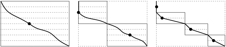
(Figure 7 illustrates this idea.) To solve the original problem we just call Path$(u_{0},w_{0})$ where $u_{0}=(0,0)$ and $w_{0}=(D,n-1).$ Correctness follows from the fact that at each recursive call, the vertical distance $d_{w}-d_{u}$ decreases so the recursion must terminate. Furthermore, when the recursion terminates, either (i) $u=(d,j)$ and $w=(d+1,j)$ so the only $u$-$w$ path in $G(u,w)$ is the edge $(u,w)$ or (ii) $u=(d,i)$ and $w=(d^{\prime},i)$ so the only $u$-$w$ path in $G(u,w)$ is the vertical path going down from $u$ to $w$.

The efficiency of the resulting algorithm, both in time and space, will depend upon how efficiently $v=Mid(u,w)$ can be found. Note that with the exception of the calls of type $Mid(u,w)$, the rest of the execution of Path$(u_{0},w_{0})$ (including all recursive calls) only requires a total of $O(D)$ space, since each recursive call uses only $O(1)$ space and there are at most $O(D)$ such calls. Thus, if $Mid(u,w)$ can be found using $O(n+D)$ space, then the entire procedure requires only $O(n+D)$ space. This is actually how both [26, 25] achieve their space bounds. The two algorithms differ in how they calculate $v$. Although both their approaches can be used for our problem, we will work with a modified version of that of [25], since it will be simpler to explain.

We now describe how to use the SMAWK algorithm to find $Mid(u_{0},w_{0})$ in $O(nD)$ time and $O(n)$ space. The extension to general $Mid(u,w)$ will follow later. Recall that the procedure Fill_Table from Figure 4 used the fact that $H(\cdot,\cdot)$ was Monge and the SMAWK algorithm to iteratively fill in the rows $H(d,\cdot)$, for $d=1,2,\ldots,D.$ Given row $H(d-1,\cdot)$, the procedure calculated $H(d,\cdot)$ in $O(n)$ time using SMAWK, and then threw away $H(d-1,\cdot)$.

Consider an arbitrary node $(d,i)$ on level $d>\bar{d}.$ The shortest path from $u_{0}$ to $(d,i)$ must pass through some node on level $\bar{d}$. We now modify Fill_Table to “remember” this node. More specifically, our algorithm will calculate auxiliary data $pred(d,i)$.

• •

  For $d<\bar{d}$, $pred(d,i)$ will be undefined.

• •

  For $d\geq\bar{d}$, $pred(d,i)$ will be an index $j$ such that node $(\bar{d},j)$ appears on some shortest path from $u_{0}$ to $(d,i)$.

So, when the procedure terminates, $v=(\bar{d},\,pred(d,n-1))$ will be $Mid(u_{0},w_{0}).$

By definition, on level $\bar{d}$, we have $pred(\bar{d},i)=i.$

For $d>\bar{d}$ suppose $(d-1,j^{\prime})$ is the immediate predecessor of $(d,i)$ on the shortest path from $u_{0}$ to $(d,i)$. Then (i) a shortest path from $u_{0}$ to $(d-1,j^{\prime})$ followed by (ii) the edge from $(d-1,j^{\prime})$ to $(d,i)$ is (iii) a shortest path from $u_{0}$ to $(d,i)$; we may therefore set $pred(d,i)=pred(d-1,j^{\prime}).$

We can use this observation to modify Fill_Table to calculate the $pred(d,\cdot)$ information.

Note that $Mid(u_{0},w_{0})$ can throw away all of the values $pred(d-1,\cdot)$ and $H(d-1,\cdot)$ after the values $pred(d,\cdot)$ and $H(d,\cdot)$ have been calculated, so it only uses $O(n)$ space. Similarly to the analysis of Fill_Table, it uses only $O(nD)$ time since each call to the SMAWK algorithm uses only $O(n)$ time.

So far, we have only shown how to find $v=Mid(u_{0},w_{0})$. Note that the only assumptions we used were that $H(\cdot,\cdot)$ satisfies DP (2) and is Monge, i.e., the $c^{(d)}_{i,j}$ satisfy (7).

Now suppose that we are given

$G(u,w)$ is a dropping level-graph on its own nodes so the cost of the shortest path from $u$ to any node $(d_{u}+d,i_{u}+i)\in G(u,w)$ is $\tilde{H}(d,i)$ defined by

where $N=i_{w}-i_{u}+1$ and $\tilde{c}^{(d)}_{i,j}=c^{(d)}_{i_{u}+i,i_{u}+j}.$ Note that this new DP is exactly in the same form as (2), just with a different $n$ and shifted $c^{(d)}_{i,j}.$ Since the original $c^{(d)}_{i,j}$ satisfy (7), so do the $\tilde{c}^{(d)}_{i,j}$. Thus (9) with the $\tilde{c}^{(d)}_{i,j}$ is Monge as well.

Therefore, we can run exactly the same algorithm written in Figure 8 to find the midpoint $v=(\bar{d},\bar{i})=Mid(u,w),$ of the min-cost $u$-$w$ path in $O((d_{w}-d_{u})N)$ time and $O((d_{w}-d_{u})+N)=O(D+n)$ space.

As discussed previously, if $Mid(u,w)$ only requires $O(n+D)$ space, then Path$(u,w)$ only requires $O(n+D)$ space, so we have completed the space analysis.

It remains to analyze running time. Set

to be the “area” of $G(u,w)$. Recall that line 3 of Path$(u,w)$implies that $d_{u}\not=d_{w}$ when $Mid(u,w)$ is called. Therefore $N\geq 1$ and the running time of $Mid(u,w)$ is

We now analyze the running time of Path$(u_{0},w_{0})$. First consider the recursive calls when lines 1-4 occur, i.e., the recursion terminates. The total work performed by such calls is the total number of edges outputted. Since an edge is outputted only once and the total path contains $D$ edges, the total work performed is $O(D).$

Next consider the calls when line 5-7 occur. Since each such call returns a vertex $v$ on the path, there are only $D-1$ such calls so lines 6 and 7 are only called $O(D)$ times and their total work, with the exception of the call to $Mid(u,v)$, is $O(D).$

Finally consider the work performed by the $Mid(u,w)$ calls. Partition the calls into levels.

• •

  Level 1 is the original call $Mid(u_{0},w_{0})$.

• •

  Level 2 contains the recursive calls directly made by the level-1 call.

• •

  In general, level $i$ contains the recursive calls directly made by the level-$(i-1)$ calls.

Note that if $Mid(u,w)$ is a level $i$ call with $u=(d_{u},i_{u})$ and $w=(d_{w},i_{w})$) then

Furthermore, by induction, if $Mid(u,w)$ and $Mid(u^{\prime},w^{\prime})$ are two different level $i$ calls, then horizontal ranges $[d_{u},d_{w}]$ and $[d_{u^{\prime}},d_{w^{\prime}}]$ are disjoint except for possibly $d_{w}=d_{u^{\prime}}$ or $d_{u}=d_{w^{\prime}}$.

Fix $i.$ Let $(u_{j},w_{j})$ $j=1,\ldots t$ be the calls at level $i$. The facts that each grid $G(u_{j},w_{j})$ has height $\leq\frac{D}{2^{i}}+1$ and that the horizontal ranges of the grids are disjoint implies

Thus the total of all level-$i$ calls is $O\left(n\left(\frac{D}{2^{i}}+1\right)\right)$. Summing over the $\lceil\log D\rceil$ levels we get that the total work performed by all of the $Mid(u,w)$ calls on line 6 is

Thus, the total work performed by Path$(u_{0},w_{0})$ is $O(nD)$ and we are finished.

We just saw how, in $\Theta(nD)$ time and $\Theta(n+D)$ space, to solve the construction problem for any DP in form (2) that satisfies the Monge property (7). $\Theta(nD)$ time was known previously; the $\Theta(n+D)$ space bound, is the new improvement. There are many other DP problems besides the binary LLHC that satisfy (7) and whose space can thus be improved. We illustrate with three examples.

We also mention that there is an undirected variant of this problem in which a node is serviced by its closest service center looking both left and right. There are many algorithms in the literature that (explicitly or implicitly) use concavity to construct solutions for this problem in $O(nD)$ time using $O(n)$ space, e.g., [29, 30, 31]. [31] does this by using a DP formulation that is in the DP form (2) and satisfies the Monge property (7) so the technique in this paper can reduce the space for this problem down to $O(n)$ as well.

References

- [1] D. A. Huffman, “A method for the construction of minimum-redundancy codes,” in Proceedings of the Institution of Radio Engineers, vol. 40, 1952, pp. 1098–1101.
- [2] J. van Leeuwen, “On the construction of huffman trees,” in Proceedings of the 3rd International Colloquium on Automata, Languages and Programming, 1976, pp. 382–410.
- [3] R. M. Karp, “Minimum-redundancy coding for the discrete noiseless channel,” IEEE Transactions on Information Theory, vol. 7, no. 1, pp. 27–38, 1961.
- [4] E. N. Gilbert, “Codes based on inaccurate source probabilities,” IEEE Transactions on Information Theory, vol. 17, no. 3, pp. 304–314, 1971.
- [5] T. C. Hu and K. C. Tan, “Path length of binary search trees,” SIAM Journal on Applied Mathematics, vol. 22, no. 2, pp. 225–234, 1972.
- [6] M. R. Garey, “Optimal binary search trees with restricted maximal depth,” SIAM Journal on Computing, vol. 3, no. 2, pp. 101–110, 1974.
- [7] D. E. Knuth, “Optimum binary search trees,” Acta Informatica, vol. 1, pp. 14–25, 1971.
- [8] L. L. Larmore, “Height restricted optimal binary trees,” SIAM Journal on Computing, vol. 16, no. 6, pp. 1115–1123, 1987.
- [9] L. L. Larmore and D. S. Hirschberg, “A fast algorithm for optimal length-limited Huffman codes,” Journal of the ACM, vol. 37, no. 3, pp. 464–473, 1990.
- [10] N. Megiddo, “Applying parallel computation algorithms in the design of serial algorithms,” Journal of the ACM, vol. 30, no. 4, pp. 852–865, 1983.
- [11] A. Aggarwal, B. Schieber, and T. Tokuyama, “Finding a minimum-weight -link path in graphs with the concave Monge property and applications,” Discrete and Computational Geometry, vol. 12, pp. 263–280, 1994.
- [12] B. Schieber, “Computing a minimum weight -link path in graphs with the concave Monge property,” Journal of Algorithms, vol. 29, no. 2, pp. 204–222, 1998.
- [13] A. Turpin and A. Moffat, “Efficient implementation of the package-merge paradigm for generating length-limited codes,” in Proceedings of Computing: The Australasian Theory Symposium, 1996, pp. 187–195.
- [14] ——, “Practical length-limited coding for large alphabets,” The Computer Journal, vol. 38, no. 5, pp. 339–347, 1995.
- [15] L. L. Larmore and T. M. Przytycka, “Parallel construction of trees with optimal weighted path length,” in Proceedings of the 3rd Annual ACM Symposium on Parallel Algorithms and Architectures, 1991, pp. 71–80.
- [16] ——, “Constructing huffman trees in parallel,” SIAM Journal on Computing, vol. 24, no. 6, pp. 1163–1169, 1995.
- [17] G. J. Woeginger, “Monge strikes again: Optimal placement of web proxies in the Internet,” Operations Research Letters, vol. 27, no. 3, pp. 93–96, 2000.
- [18] B. Krishnamachari, R.-H. Gau, S. B. Wicker, and Z. J. Haas, “Optimal sequential paging in cellular wireless networks,” Wireless Networks, vol. 10, no. 2, pp. 121–131, 2004.
- [19] P. Bradford, M. J. Golin, L. L. Larmore, and W. Rytter, “Optimal prefix-free codes for unequal letter costs: Dynamic programming with the Monge property,” Journal of Algorithms, vol. 42, no. 2, pp. 277–303, 2002.
- [20] R. Wilber, “The concave least-weight subsequence problem revisited,” Journal of Algorithms, vol. 9, no. 3, pp. 418–425, 1988.
- [21] A. Aggarwal, M. M. Klawe, S. Moran, P. W. Shor, and R. E. Wilber, “Geometric applications of a matrix-searching algorithm,” Algorithmica, vol. 2, pp. 195–208, 1987.
- [22] D. Eppstein, “Smawk totally monotone matrix searching algorithm,” Python Package available at: http://aspn.activestate.com/ASPN/Cookbook/Python/Recipe/117244, 2002, release March 17, 2002.
- [23] “Neobio bioinformatics algorithms in java: Class smawk,” Java Package available at: http://neobio.sourceforge.net/javadoc/neobio/alignment/Smawk.html.
- [24] R. E. Burkard, B. Klinz, and R. Rudolf, “Perspectives of Monge properties in optimization,” Discrete Applied Mathematics, vol. 70, no. 2, pp. 95–161, 1996.
- [25] J. I. Munro and R. J. Ramirez, “Reducing space requirements for shortest path problems,” Operations Research, vol. 30, no. 5, pp. 1009–1013, 1982.
- [26] D. S. Hirschberg, “A linear space algorithm for computing maximal common subsequences,” Communications of the ACM, vol. 18, no. 6, pp. 341–343, 1975.
- [27] K.-M. Chao, R. C. Hardison, and W. Miller, “Recent developments in linear-space alignment methods: A survey,” Journal of Computational Biology, vol. 1, no. 4, pp. 271–292, 1994.
- [28] E. W. Myers and W. Miller, “Optimal alignments in linear space,” Bioinformatics (formerly Computer Applications in the Biosciences), vol. 4, no. 1, pp. 11–17, 1988.
- [29] R. Hassin and A. Tamir, “Improved complexity bounds for location problems on the real line,” Operations Research Letters, vol. 10, no. 7, pp. 395–402, 1991.
- [30] V. Auletta, D. Parente, and G. Persiano, “Placing resources on a growing line,” Journal of Algorithms, vol. 26, no. 1, pp. 87–100, 1998.
- [31] R. Fleischer, M. J. Golin, and Y. Zhang, “Online maintenance of k-medians and k-covers on a line.” Algorithmica, vol. 45, no. 4, pp. 549–567, 2006.
- [32] B. Krishnamachari, R.-H. Gau, S. B. Wicker, and Z. J. Haas, “Optimal sequential paging in cellular wireless networks,” Wireless Networks, vol. 10, no. 2, 2004.
- [33] A. Bar-Noy, M. J. Golin, and Y. Zhang, “Online dynamic programming speedups,” in Proceedings of the 4th Workshop on Approximation and Online Algorithms, 2006.
- [34] L. L. Larmore and B. Schieber, “On-line dynamic programming with applications to the prediction of RNA secondary structure,” Journal of Algorithms, vol. 12, no. 3, pp. 490–515, 1991.
Appendix A Derivation of the LLHC Dynamic Program
In order to make this note self-contained we provide a brief derivation of the DP that models the LLHC. To the best of our knowledge, the derivation for the general -ary case has never been written down before (although it is known as “folklore”).
A set of prefix-free codes in an -ary alphabet can be represented by an -ary tree with leaves. The edge from an internal node to its children is labeled by . Each leaf corresponds to a code word, which is the concatenation of the characters on the root-to-leaf path. Then, the expected code length equals the weighted external path length of the tree.
Denote the height of the tree by . The lowest leaves are on level ; the root is at level . Optimal (min weighted external path-length) assignments of the probability ’s to the leaves always assign smaller probabilities to leaves at lower levels. Since the probabilities are given in sorted order, this assignment can be done in time for a given tree. The cost of a tree is its weighted external path length w.r.t. an optimal assignment.
Define the degree of a node to be the number of its children. A node is complete if it is of degree , and a tree is complete if all its internal nodes are complete. The following properties are easy to prove
Property 1
In an optimal tree, the internal nodes at levels are complete.
Property 2
There is an optimal tree that has at most one incomplete internal node, and if this node exists, it is at level . Furthermore, the degree of this incomplete node is .
These properties imply that the optimal tree is almost complete and has internal nodes. If is divisible by , the tree is complete. Otherwise, we can add
dummy leaves to make it complete. We assign dummy ’s with zero values to these dummy leaves. It is easy to see that the new tree with these dummy leaves is precisely an optimal tree for the probabilities with the added zero-valued dummy ’s. So, finding an optimal tree for probabilities with these dummy ’s is equivalent to the original problem. Therefore, w.l.o.g., we assume in the original problem, the optimal tree is a complete tree, i.e., we assume is always a multiple of . In this way we transform the -ary Huffman coding problem to the problem of finding an optimal complete -ary tree with leaves.
A complete tree of height can be fully represented by a sequence , where denotes the number of internal nodes at levels . Note that from this sequence we can calculate , the number of internal nodes on level and with that information we can reconstruct the tree in time as follows:
Create
1. For to
2. Create nodes on level ;
3. Create leaves on level ;
4. Make the parents of the nodes on
level .
We will now see how to rewrite the cost of a tree using its representative sequence:
Lemma 5
If represents tree , then has leaves on levels
Proof:
Consider the forest which is the portion of on or below level . It is composed of trees with roots on level ,
In total, the forest contains internal nodes.
If is a complete -ary tree with internal nodes then has leaves so our forest must contain leaves. ∎
Recall that for . Using the lemma above, we have
Lemma 6
If the sequence represents a tree, then the cost of the tree is .
For a complete -ary tree with leaves, we have and, from Lemma 5, for all .
For technical reasons, because we will be dealing with trees having height at most (but not necessarily equal to) , we allow initial padding of the sequence by 0s so that a sequence representing a tree will be of the form that has the following properties
Definition 5
A sequence is a valid -sequence, if
- •
such that
for all .
A sequence is complete if it is valid and .
It is straightforward to see that padding the sequence representing a tree with initial 0s, does not change the tree built by the Create procedure or the validity of Lemmas 5 and 6.
We can now extend our cost function to all valid -sequences sequences, not just the ones representing trees.
Definition 6
For valid -sequence define
is optimal if where the minimum is taken over all valid length -sequences with i.e., all sequences of the same length that end with the same value.
Note: padding a sequence with initial 0s doesn’t change its completeness or cost. Furthermore, if is created by padding the sequence corresponding to tree with initial 0s, then procedure Create will still recreate from
It follows from the definitions that for fixed we can calculate , the cost of an optimal -sequence with using the DP (2) with