Suppression of non-adiabatic phases by a non-Markovian environment:
easier observation of Berry phases.

We consider a spin-half coupled to an environment via a coupling axis, ${\bf e}(t)$, which is rotated around a closed loop (see Fig. 1a). The total Hamiltonian for the system (sys) and its environment (env) is

with $\hat{\mbox{\boldmath${\sigma}$}}=(\hat{\sigma}_{x},\hat{\sigma}_{y},\hat{\sigma}_{z})$ being the vector of Pauli matrices. The unit vector ${\bf e}(t)$ is slowly rotated around a closed loop. The operators $\hat{a}_{j}^{\dagger}$ and $\hat{a}_{j}$, create and destroy the $j$th excitation of the environment, where ${\cal H}_{\rm env}\big(\{\hat{a}_{j}^{\dagger},\hat{a}_{j}\}\big)$ is such that the $j$th excitation has energy $\Omega_{j}$. Note that this is a model of a degenerate two-level system coupled to an environment, because we require that the two-level system’s Hamiltonian is zero if one takes ${\cal H}_{\rm int}\to 0$ (we relax this requirement in Section VI).

We assume that the environment has a spectrum such that it is highly non-Markovian; by which we mean that the environment has a significant effect on the system’s dynamics on a timescale much less than the environment’s memory time, $\tau_{\rm mem}$. This memory time is defined as the timescale on which $\sum_{j}\langle\hat{a}_{j}^{\dagger}(\tau)\hat{a}_{j}(0)\rangle$ decays, where $\hat{a}_{j}^{\dagger}(\tau),\hat{a}_{j}(\tau)$ are creation and annihilation operators in the interaction picture, so that $\hat{a}_{j}^{\dagger}(\tau)=\exp[{-{\rm i}{\cal H}_{\rm env}\tau}]\hat{a}_{j}^{\dagger}\exp[{{\rm i}{\cal H}_{\rm env}\tau}]$.

Here we say that any zero temperature environment is highly non-Markovian when the dimensionless environment-coupling parameter

where $\Omega_{\rm m}$ is the average frequency of the environment; defined by $\Omega_{\rm m}=\left(\sum_{j}K_{j}^{2}\Omega_{j}\right)/\left(\sum_{j}K_{j}^{2}\right)$. For an environment of harmonic oscillators this can be generalized to arbitrary environment temperature, $T$; such an environment is highly non-Markovian if

where $\beta=(k_{\rm B}T)^{-1}$. We have in mind an environment containing so many modes with different frequencies that the sum can be written as an integral as in Eq. (29).

To get a feeling for such an environment, it is worth considering an environment at zero temperature with $N$ modes each coupled to the system with a strength $K$, and with frequencies spread around an average of $\Omega_{\rm m}$. For simplicity we assume that the spread of frequencies is also of order $\Omega_{\rm m}$, in such a case ${G_{\rm dis}}\simeq NK^{2}/\Omega_{\rm m}^{2}$. One can then see that ${G_{\rm dis}}\ll 1$ corresponds to an approximately Markovian environment by looking at the derivation of the Bloch-Redfield master equation [19, 20] which has a Markovian form (see for example Ref. 21). There the memory time $\tau_{\rm mem}\sim\Omega_{\rm m}^{-1}$, while the rate at which the environment affects the system’s dynamics is $\Gamma\sim NK^{2}\tau_{\rm mem}$. The Bloch-Redfield approximation is then applicable when $\Gamma\tau_{\rm mem}\ll 1$; then spin relaxation and dephasing times (known as $T_{1}$ and $T_{2}$ respectively) are of order $\Gamma^{-1}$ so $\tau_{\rm mem}\ll T_{1,2}$. This corresponds to ${G_{\rm dis}}\ll 1$. In contrast the Lindblad equation master equation [17, 18, 21] is only applicable when $\tau_{\rm mem}\to 0$ (strictly Markovian environment) with $NK^{2}$ scaled so that $\Gamma$ remains finite. This therefore corresponds to ${G_{\rm dis}}=0$.

In this work we consider exactly the opposite limit, ${G_{\rm dis}}\gg 1$. One might guess that this corresponds to dephasing so strong that it occurs in a time shorter than the environment memory time. However in this regime relaxation and dephasing rates are not given by the above $\Gamma$. Instead there is extremely strong renormalization of the system’s dynamics with relatively weak relaxation and dephasing.

Most works on systems coupled to environments have considered that the environment is made up of harmonic oscillators. We do the same here, treating ${\cal H}_{\rm env}=\sum_{j}\Omega_{j}\hat{a}_{j}^{\dagger}\hat{a}_{j}$ (up to an irrelevant constant that we neglect). This enables us get closed form expression for finite temperatures without too much difficulty. However, we emphasis that the low temperature limit of our results are applicable to any large environment, for example an environment made of two-level systems.

To see why this is so, consider any large environment which is initially in its ground-state. The analysis that follows in this article assumes that the system only weakly interacts with each degree-of-freedom in the environment, The effect of the environment on the system is none the less strong because there are so many degrees-of-freedom in the environment. Thus the interaction with each environment degree-of-freedom can be treated to lowest order. This means that the interaction can only take environment mode $j$ from its ground state to its first excited state. In this case the only property of environment mode $j$ that is relevant to the system’s evolution is the gap between its ground state and its first excited state, which we define as $\Omega_{j}$. Thus, for temperatures such that ${\rm e}^{-\beta\Omega_{j}}\ll 1$ for the vast majority of $j$, the nature of environment modes is strictly irrelevant,; they could be harmonic oscillators (with an infinite ladder of equally spaced excited states), spin-halves (with no states beyond the first excited state), or any other quantum systems.

Thus one can expect that the $\beta\Omega_{\rm m}\gg 1$ limit of all results in this article will apply to arbitrary environments, while the results for arbitrary $\beta$ only apply to an environment of harmonic oscillators.

One can map the dynamics of a system coupled to an environment of quantum oscillators at infinite temperatures onto the ensemble-averaged dynamics of a system coupled to classical noise [16]. Thus we also analyze the problem of a spin subject to classical noise (with $N$ components) when the noise axis is rotated (see Fig. 1b). In Section V, we discuss what happens to a spin whose Hamiltonian is given by

when the unit vector ${\bf e}(t)$ is slowly rotated around a closed loop, and $A_{j},\phi_{j}$ are random. The amplitude $A_{j}$ is gaussianly distributed with variance $\langle A_{j}^{2}\rangle$, and $\phi_{j}$ is uniformly distributed over all angles from $0$ to $2\pi$.

The mapping from the quantum environment to classical noise tells us that the average system dynamics under ${\cal H}_{\rm cl}$ is given by taking the infinite temperature limit ($\beta=(k_{\rm B}T)^{-1}\to 0$) of the system’s dynamics under ${\cal H}_{\rm sys\&env}$ when the environment consists of harmonic oscillators and $K_{j}^{2}$ is replaced by $\beta\Omega_{j}\langle A_{j}^{2}\rangle$. Thus for such classical noise we can define the noise-coupling parameter

Here, we consider only highly non-Markovian classical noise for which ${G_{\rm dis}}\gg 1$.

When one performs a Berry phase experiment on a system (rotating its Hamiltonian around a closed path), one can rarely ignore the coupling to an environment (or noise). Despite hints to the contrary [22], noise-induced fluctuations of $\Phi_{\rm dyn}$ typically lead to a dephasing time, $T_{2}$, on which all phase information (including the Berry phase) is lost [23, 24, 25] (here we do not consider the intriguing use of repeatable noise in Ref. [6]). Thus a Berry phase can only be observed if one is able to adiabatically rotate the Hamiltonian around a closed loop in a time $t_{\rm p}\lesssim T_{2}$. Usually this requires $T_{2}\gtrsim t_{\rm p}\gg E^{-1}$, where $E$ is the energy gap to system excitations [10]. The environment also modifies the Berry phase [23]; the modification is geometric (quadrupole-like) and complex [26, 27] (see also [28]), with its imaginary part being geometric dephasing.

Ref. [29] made the remarkable observation that a time-dependence in the coupling to an environment could also generate a Berry phase (see also [30, 31]). Dissipative processes (at a rate $T_{2}^{-1}$) cause the system state to adiabatically follow the time-dependence of the system-environment coupling, thereby acquiring a Berry phase. In Ref [29], unlike in our Eq. (2), there are non-adiabatic corrections of the form $\Phi_{\rm NA}^{(\mu)}\sim(t_{\rm p}/T_{2})^{-\mu}$ for all integer $\mu\geq 1$. To avoid the non-adiabatic effects, one requires that $t_{\rm p}\gg T_{2}$, which means that dephasing occurs long before the rotation is completed. Thus this Berry phase can only be observed for states in a decoherence-free subspace [29].

All the works listed above considered Berry phases in systems coupled to environments or classical noise that were strictly or approximately Markovian. In contrast, in this article we consider a highly non-Markovian environment, which strongly renormalizes the system dynamics without causing significant dissipation. The adiabatic evolution is ensured by this renormalization (not dissipation), and it leads to Eq. (2). The relative lack of dissipation means that there is no need to use a decoherence-free subspace.

Neither the Lindblad nor Bloch-Redfield methods, used to study Berry phases in Refs. [29, 30] and Ref. [31] respectively, can capture the strong renormalization that occurs for ${G_{\rm dis}}\gg 1$. The Lindblad master equation applies for ${G_{\rm dis}}=0$, while the Bloch-Redfield master method applies for ${G_{\rm dis}}\ll 1$, which corresponds to only a very small linear renormalization effect.

We conclude by mentioning a number of works in chemical physics. Berry phases occur in molecular dynamics because there is a separation of timescales; the nuclei are heavy and move slowly, while the electrons are light and move fast. This makes it natural to perform a Born-Oppenheimer decoupling of the fast and slow degrees-of-freedom. It is well-known that such a de-coupling can lead to a Berry phase, see for example Refs. [2, 3]. There are also non-adiabatic corrections to this Berry phase which come from violations of the Born-Oppenheimer decoupling. These have been well studied; for an older review see Ref. [32] and references therein, for more recent work see Ref. [33]. However all the works that we are aware of, consider only a relatively small number of degrees-of-freedom (for example a tri-atomic molecule, containing three slow nuclear degrees of freedom and up to three fast electron degrees-of-freedom). In this article, we also go beyond the Born-Oppenheimer approximation to find the non-adiabatic corrections to the Berry phase. However we are interested in a two-level system (qubit) which is very weakly coupled to each of an enormous number of environment modes (or classical noise modes), such that the combined effect of all these modes on the system dynamics is very strong. This is the opposite limit from that considered in the works on molecular dynamics.

To deal with a problem in which the axis the environment couples to is rotating with time (as sketched in Fig. 1), we go to a rotating basis [9] whose $z$-axis remains parallel to ${\bf e}(t)$. We transform to such a basis using ${\cal U}=\exp(-i{\textstyle\frac{1}{2}}\varphi\hat{\sigma}_{z})\exp(i{\textstyle\frac{1}{2}}\theta\hat{\sigma}_{y})\exp(i{\textstyle\frac{1}{2}}\varphi\hat{\sigma}_{z})$, in terms of polar coordinates ${\bf e}(t)=(\theta,\varphi)$. This choice of ${\cal U}$ gives ${\cal U}({\bf e}(t)\cdot\hat{\mbox{\boldmath${\sigma}$}}){\cal U}^{\dagger}=\hat{\sigma}_{z}$ while having no ambiguity for $\theta=0$. In this basis, the Hamiltonian has an extra magnetic field equal to the basis’ angular velocity[10], ${\omega}$, thus it is given by

where the angular velocity in this rotating basis is

For convenience in what follows, we define $\omega_{\perp}$ as the magnitude of the component of $\omega$ that is perpendicular to the environment-coupling axis, then

Thus to summarizing the situation, we have removed the time-dependence from the coupling to the environment, by going to the rotating frame. The Hamiltonian in Eq. (8) is a biased spin-boson model (with the environment coupling to the spin’s $z$-axis) and thus we can proceed to treat it via a polaron transformation in a similar manner to Refs. [35, 36, 37, 38, 39].

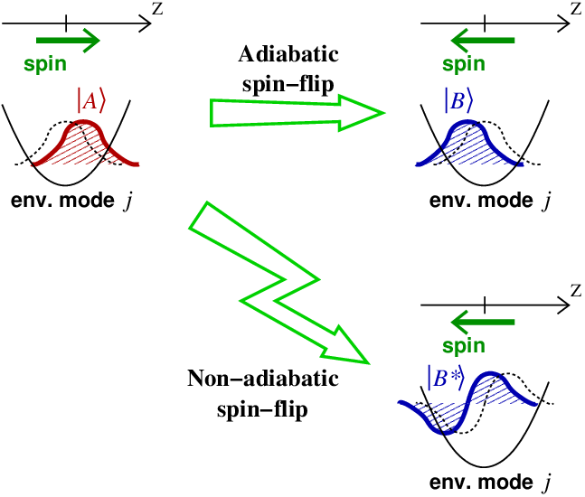
The physics behind the polaron transformation is the idea that fast environment modes tend to adiabatically follow the slow system modes, so they can be thought of as a “cloud” around the system, renormalizing its dynamics. So we go to the basis of this “cloud”, by writing ${\cal H}_{\rm sys\&E}^{\rm rot}$ in terms of a new (orthonormal) set of basis-states in which environment modes are shifted due to the force induced by the spin being $\uparrow$ or $\downarrow$. A cartoon of this (for a single environment mode) is shown in Fig. 2.

In this basis of shifted environment modes, any wave-function can be written as

where $|m_{j}^{\uparrow}\rangle$ indicates that the $j$th environment mode is in the $m$th eigenstate of the shifted Hamiltonian $\hat{\cal H}_{j}^{\rm shift;\uparrow}=K_{j}(\hat{a}_{j}^{\dagger}+\hat{a}_{j})/2+\Omega_{j}\hat{a}_{j}^{\dagger}\hat{a}_{j}$ (we drop an irrelevant constant term). Similarly $|m_{j}^{\downarrow}\rangle$ is the $m$th eigenstate of $\hat{\cal H}_{j}^{\rm shift;\downarrow}$, given by $\hat{\cal H}_{j}^{\rm shift;\uparrow}$ with $K_{j}\to-K_{j}$. We assume that each environment mode is only weakly affected by the system, $K_{j}\ll\Omega_{j}$, then the difference between $|m_{j}^{\uparrow}\rangle$ and $|m_{j}^{\downarrow}\rangle$ is small. Defining $\alpha_{j}\equiv(K_{j}/\Omega_{j})$, one finds,

where $\alpha_{j}=K_{j}/\Omega_{j}$. The higher the level, $m_{j}$, of the initial state of the $j$th environment mode, the smaller this overlap is. While this overlap is very close to one, the fact that it is slightly less than one can have a huge effect on the system, because there are many such overlaps. Each time the spin-flips it must carry the “cloud” of environment modes with it, as a result the spin-flip rate is multiplied by the product over all $j$ of the above overlaps; this product of $N$ overlaps — each of which is slightly less than one — will decay exponentially with $N$. Thus for large $N$, the $N$-particle environment state after the spin-flip will be almost orthogonal to the $N$-particle environment state before the spin-flip. This means that the matrix element for spin-flips is suppressed (becoming exponentially small in $N$). Such a suppression is often called the Anderson orthogonality catastrophe [12], since he pointed out that it can strongly suppress the tunnelling of an electron between two metals electrode [40].

Intriguingly the higher the level, $m_{j}$, of the initial state of the $j$th environment mode, the further the overlap in Eq. (18) is from one. This would imply that the orthogonality catastrophe is stronger at higher temperatures. However this view is too simplistic, because it neglects possible excitations of the “cloud” of environment modes that follow the spin. The overlaps which correspond to such excitations are

Note that if we flip all the spins ($\uparrow\leftrightarrow\downarrow$) in Eq. (19), then the right-hand-side changes sign. We will see that these effects tend to counteract the orthogonality catatrophy which occurs in the adiabatic evolution. Thus we must take seriously their contributions to the dynamics.

We transform Eq. (8) to the basis of shifted environment-modes, using a polaron transformation [34, 35, 36]; for completeness we explain the transformation in Appendix B. The transformed Hamiltonian is

The non-interacting Hamiltonian, $({\cal H}^{\prime}_{\rm sys}+{\cal H}^{\prime}_{\rm env})$, involves no transitions of the environment modes; thus it gives adiabatic evolution. The interaction term, ${\cal V}$, contains all non-adiabatic effects (i.e. transitions between environment states). The first term in ${\cal V}$ involves transitions of an even (non-zero) number of environment modes, while the second involves transitions of an odd number of environment modes. The Hermitian operators ${\cal Q}_{\rm even,odd}$ are

where ${\cal R}_{\pm}={\prod_{j}}\big[1\pm\alpha_{j}\hat{\sigma}^{\prime}_{z}(\hat{a}_{j}^{\prime\dagger}-\hat{a}^{\prime}_{j})\big].$ The exponential suppression of perpendicular fields in ${\cal H}^{\prime}_{\rm sys}$ is given by the Franck-Condon factor,

If the environment consists of harmonic oscillators at temperature $T$, then $F={\textstyle\frac{1}{2}}\sum_{j}\alpha_{j}^{2}\,\coth\big(\beta\Omega_{j}/2\big)$, where $\beta=(k_{\rm B}T)^{-1}$ (see Appendix B).

We can make a Born-Oppenheimer (BO) approximation of Eq. (20), by simply neglecting ${\cal V}$ (since it excites environment modes). Such a BO decoupling of fast modes (environment) from slow modes (system) is known to create Berry phases [3]. A priori, one might guess that this BO approximation is justified when the rotation-rate, $\omega$, is small enough that $\omega\ll\Omega_{\rm m}$. Below we find the non-adiabatic corrections and show a posteriori that in fact the BO approximation is valid when $\omega\ll\Omega_{\rm m}{G_{\rm dis}}^{1/2}$. For the non-Markovian environments that we consider here (${G_{\rm dis}}\gg 1$), this condition is much less stringent that the above guess.

In the BO approximation, the spin-dynamics are simply given by ${\cal H}^{\prime}_{\rm sys}$. Assuming the Franck-Condon factor is large, we can neglect all terms which go like ${\rm e}^{-F}$, then the Hamiltonian is simply $-{\textstyle\frac{1}{2}}\omega_{z}\hat{\sigma}^{\prime}_{z}$. The off-diagonal terms in this adiabatic Hamiltonian are exponentially suppressed, due to the Anderson orthogonality catastrophe [12] as outlined above. Thus the spin adiabatically follows ${\bf e}(t)$, and the total phase acquired by the spin is $\pm{\textstyle\frac{1}{2}}\int_{0}^{t_{\rm p}}{\rm d}t\,\omega_{z}$ where $\pm$ are for $\uparrow,\downarrow$. To observe this phase, we study the precession of a superposition of $\uparrow$ and $\downarrow$, this precession is given by the phase difference between $\uparrow$ and $\downarrow$, which is $\Phi_{\rm total}=\int_{0}^{t_{\rm p}}{\rm d}t\,\omega_{z}$ This equals the Berry phase,

where ${\cal A}$ is the solid-angle enclosed by the path of ${\bf K}(t)$. Following Berry, we can write this as $\oint\!{\bf a}\,{\rm d}{\bf K}$, and use Stokes’ theorem to give $\Phi_{\rm BP}=\int{\bf b}\,{{\rm d}{\bf S}}$ where ${\bf b}\equiv{\bf\nabla}_{\bf K}\times{\bf a}$ is Berry’s monopole-field, $(b_{K},b_{\theta},b_{\varphi})=(K^{-2},0,0)$.

This BO analysis is sufficient to show that the spin acquires a Berry phase, and that there is no dynamic phase, $\Phi_{\rm dyn}$. However to see the form of the non-adiabatic phases, we have to go beyond the BO approximation.

References

- [1] M.V. Berry, Proc. R. Soc. Lond. 392, 45 (1984).
- [2] A. Shapere and F. Wilczek (Eds.), Geometric phases in physics (World Scientific, Singapore, 1989).
- [3] C.A. , Rev. Mod. Phys. 64, 51 (1992).
- [4] J. Anandan, J. Christian and K. Wanelik, Am. J. Phys. 65 180 (1997).
- [5] P.J. Leek et al, Science 318, 1889 (2007).
- [6] S. Filipp, J. Klepp, Y. Hasegawa, C. Plonka-Spehr, U. Schmidt, P. Geltenbort, and H. Rauch,Phys. Rev. Lett. 102, 030404 (2009)
- [7] J.A. Jones, V. Vedral, A. Ekert and G. Castagnoli, Nature 403, 869 (2000). A. Ekert et al, J. Mod. Opt. 47, 2501, (2000).
- [8] J.P. Pekola, J.J. Toppari, M. Aunola, M.T. Savolainen and D.V. Averin, Phys. Rev. B 60, R9931 (1999). R. Leone, L.P. Lévy and P. Lafarge, Phys. Rev. Lett. 100, 117001 (2008).
- [9] M.V. Berry, Proc. R. Soc. Lond. A, 414, 31 (1987).
- [10] We gives all energies and B-fields in units of inverse time.
- [11] F. Wilczek and A. Zee, Phys. Rev. Lett. 52, 2111 (1984).
- [12] P.W. Anderson, Phys. Rev. Lett. 18, 1049 (1967).
- [13] A.J. Leggett, S. Chakravarty, A.T. Dorsey, M.P.A. Fisher, A. Garg, and W. Zwerger, Rev. Mod. Phys. 59, 1 (1987), in particular Sect. IIIC.
- [14] In earlier preprints of this work (e.g. arXiv:0806.4897v1), we analyzed this problem with the adiabatic renormalization group (RG) method [13]. It gave exponential suppression of non-adiabatic phases, missing the powerlaw behaviour that we find here. The problem appears to be with so-called irrelevant terms which are usually dropped from the RG flow. They are extremely hard to sum within the RG method, however we started to suspect that they gave a contribution of order , which would typically dominate over the exponentially small rates given by the RG flow (except in the limit of ). Our suspicion led to the calculation in this article (a polaron transformation followed by standard perturbation theory rather than RG). In this approach these contributions are relatively easy to handle. This calculations confirms the existence (and importance) of the -contributions to many physical quantities. However in the language of Ref. [13], the polaron transform method is limited by being perturbative in the tunnelling rate, . We emphasis that in the special case of the quantity calculated in Ref. [13], the polaron transform method gives no -contributions (at least to leading order in ). Thus we have no reason to doubt the RG results in Ref. [13].
- [15] Y. Aharonov and J. Anandan, Phys. Rev. Lett. 58, 1593 (1987).
- [16] A.O. Caldeira and A.J. Leggett, Physica A, 121, 587 (1983). A.O. Caldeira and A.J. Leggett, Ann. Phys. (N.Y.) 149, 374(1983).
- [17] G. Lindblad, Commun. Math. Phys. 48, 119 (1976)
- [18] H.-P. Breuer and F. Petruccione, The theory of open quantum systems (Oxford University Press, Oxford, 2002).
- [19] F. Bloch, Phys. Rev. 105, 1206 (1957)
- [20] A.G. Redfield, IBM J. Res. Dev. 1, 19 (1957)
- [21] R.S. Whitney, J. Phys. A: Math. Theor. 41, 175304 (2008).
- [22] S. Lloyd, Science 292, 1669 (2001).
- [23] R.S. Whitney and Y. Gefen, Phys. Rev. Lett. 90, 190402 (2003).
- [24] G. De Chiara and G.M. Palma, Phys. Rev. Lett. 91, 090404 (2003).
- [25] M.S. Sarandy and D.A. Lidar, Phys. Rev. A 73, 062101 (2006).
- [26] R.S. Whitney, Y. Makhlin, A. Shnirman and Y. Gefen, Phys. Rev. Lett. 94, 070407 (2005).
- [27] R.S. Whitney, Y. Makhlin, A. Shnirman, Y. Gefen, NATO Science Series II: Mathematics, Physics and Chemistry, 230, 9 (2006); Eprint - arXiv:cond-mat/0401376.
- [28] X.X. Yi, L.C. Wang and W. Wang, Phys. Rev. A 71, 044101 (2005). X.X. Yi, D.M. Tong, L.C. Wang, L.C. Kwek and C.H. Oh, Phys. Rev. A 73, 052103 (2006). G. De Chiara, A. Łozinski and G.M. Palma, Eur. Phys. J. D 41, 179 (2007). F.C. Lombardo and P.I. Villar, arXiv:0802.2873. K. Fujikawa and M.-G Hu, Phys. Rev. A 79, 052107 (2009).
- [29] A. Carollo, G.M. Palma, A. Łozinski, M. Franüca Santos and V. Vedral, Phys. Rev. Lett. 96, 150403 (2006). A. Carollo and G.M. Palma, Laser Physics 16, 1595, (2006).
- [30] S. Dasgupta and D.A. Lidar, J. Phys. B: At. Mol. Opt. Phys. 40, S127 (2007).
- [31] S.V. Syzranov and Y. Makhlin, JETP Lett. 87, 390 (2008).
- [32] D.R. Yarkony, J. Phys. Chem. 100, 18612 (1996).
- [33] B.K. Kendrick,C.A. Mead and D.G. Truhlar, Chem. Phys. 277, 31 (2002).
- [34] Chapter 6 of G.D. Mahan, Many Particle Physics (Plenum Press, New York, 1981)
- [35] W. Zwerger, Z. Phys. B 53, 53 (1983). W. Zwerger, Z. Phys. B 54, 87 (1983).
- [36] R. Silbey and R.A. Harris, J. Chem. Phys. 80, 2615 (1984).
- [37] C. Aslangul, N. Pottier, and D. SaintJames, J. Physique 47 1657 (1986)
- [38] H. Dekker, Phys. Rev. A 35, 1436 (1987)
- [39] C. Aslangul, N. Pottier, and D. SaintJames, Physica A 149 535 (1988)
- [40] In this context, the electron tunnels “slowly” from a state in one metal electrode to a state in the other. The tunnelling electron repels all the other electrons in the electrodes (where they have “fast” dynamics), thus these electrons will act as a “cloud” that can strongly renormalize the tunnelling rate.
- [41] H. Schoeller and G. Schön, Phys. Rev. B 50 18436 (1994).
- [42] Y. Makhlin, G. Schön and A. Shnirman, Dissipation in Josephson qubits in New Directions in Mesoscopic Physics (Towards Nanoscience), Fazio R, Gantmakher V F, and Imry Y (Eds) (Kluwer, Dordrecht, 2003). Eprint cond-mat/0309049.
- [43] S. Nakajima, Prog. Theor. Phys. 20, 948(1958). R. Zwanzig, J. Chem. Phys. 33, 1338 (1960).
- [44] F. Haake and M. Lewenstein, Phys. Rev. A 28, 3606 (1983).
- [45] F. Haake and R. Reibold, Phys. Rev. A 32 2462 (1985).
- [46] A. Suárez, R. Silbey and I. Oppenheim, J. Chem. Phys. 97, 5101 (1992).
- [47] J. C. Garrison and E. M. Wright, Phys. Lett. A 128, 177 (1988).
- [48] P. San-Jose, G. Zarand, A. Shnirman, G. Schön, Phys. Rev. Lett. 97, 076803 (2006). R.S. Whitney, A. Shnirman and Y. Gefen, Phys. Rev. Lett. 100, 126806 (2008).
- [49] see for example : X. Wang and K. Matsumoto, J. Phys. A: Math. Gen. 34, L631 (2001).