The particle spectrum of the Tricritical Ising Model with spin reversal symmetric perturbations

The Form Factor Perturbation Theory permits to investigate the behaviour of a theory in the vicinity of an integrable direction, either if the integrable theory is massive [6, 7] or massless [8]. Let $\mathcal{A}_{\rm{int}}$ be the action of the integrable model and $\Upsilon(x)$ the field that moves the system away from integrability, so that nearby the action of the theory can be written as

$${\cal A}\,=\,{\cal A}_{\rm{int}}+\lambda\,\int\,\mathrm{d}^{2}x\,\,\Upsilon(x)\ .$$

(3.1)

If the original integrable model has scalar excitations²² 2 The rapidity variable $\theta$ expresses the dispersion relation of the excitations. If we consider a massive particle of mass $m$, its energy and momentum are given by $E=m\cosh\theta$, $p=m\sinh\theta$. If, instead, the particle is massless, it can be a right or a left mover excitation. The dispersion relations of a right mover are $E_{R}=p=M\rme^{\theta}$, while those of a left mover $E_{L}=-p=M\rme^{-\theta}$, where $M$ is an arbitrary mass scale. $A_{1}(\theta),A_{2}(\theta),\ldots$, the first order correction in $\lambda$ to their mass $M_{k}$ is given by

$$\delta M_{k}^{2}\,\simeq\,2\,\lambda\,F_{k}^{\Upsilon}(\rmi\pi)\,\,,$$

(3.2)

where

$$F_{k}^{\Upsilon}(\theta_{12})\,\equiv\,\langle 0|\Upsilon(0)|A_{k}(\theta_{1})\,A_{k}(\theta_{2})\rangle$$

(3.3)

is the two-particle form factor of the operator $\Upsilon(x)$, with $\theta_{12}=\theta_{1}-\theta_{2}$. A similar formula also holds if the integrable model has massless excitations, with a proper interpretation of the rapidity variable $\theta$ [8]. If, instead, the integrable theory has topological kinks $|K_{ab}(\theta)\rangle$ interpolating between the vacuum states $|a\rangle$ and $|b\rangle$, the relevant formula is

$$\delta M_{ab}^{2}\,\simeq\,2\,\lambda\,F_{ab}^{\Upsilon}(\rmi\pi)\,\,,$$

(3.4)

where

$$F_{ab}^{\Upsilon}(\theta_{12})\,\equiv\,_{k}\langle 0|\Upsilon(0)|K_{ab}(\theta_{1})\,K_{ba}(\theta_{2})\rangle\ .$$

(3.5)

In integrable field theories the form factors of a generic scalar operator $\Upsilon(x)$ can be computed exactly [16, 17] and therefore we can study the evolution of the spectrum near to the integrable lines. However, one has to be careful when applying the formulas (3.3) and (3.5) since the two-particle form factor can be singular at $\theta_{12}=\rmi\pi$. This happens if the perturbing operator $\Upsilon(x)$ has a semi-local index $\gamma$ with respect to the particle excitations (this is usually the case of the topological kinks, for instance). In this case the point $\theta_{12}=\pm\rmi\pi$ is the location of a simple pole of the two-particle form factor, whose residue is given by [7, 17]

$$-\rmi\,{\rm{Res}}_{\,\theta_{12}=\pm\rmi\pi}\,F_{ab}^{\Upsilon}(\theta_{12})\,=\,(1-\rme^{\mp 2\rmi\pi\gamma})\,\,_{k}\langle 0|{\Upsilon}|0\rangle_{k}\ .$$

(3.6)

The result of the brief analysis given above can be summarized as follows. If $F_{l}^{\Upsilon}(\rmi\pi)$ is finite, the corresponding particle or kink excitation survives the perturbation and its mass is adiabatically shifted from the original value. Vice versa, if $F_{l}^{\Upsilon}(\rmi\pi)$ is divergent, the corresponding excitation no longer survives as asymptotic particle of the perturbed theory, i.e. it gets confined.

The Truncated Conformal Space Approach (TCSA) [18] can be used to study perturbed conformal field theories. It consists in a finite size analysis of the spectrum of a theory on a cylinder of circumference $R$. This is realized by truncating the conformal basis at a certain level $n$ in the Verma modules of the irreducible representations of the primary fields and solving the eigenvalue and eigenvector problem of the truncated Hamiltonian operator numerically.

To extract a quantity $F$ relative to the $R\to\infty$ limiting model, one calculates $F(R,n)$ (i.e. $F$ at a cylinder circumference $R$ and truncation level $n$) for several values of $R$, and possibly also for several values of $n$. Usually there is a range $R_{F,\rm{min}}<R<R_{F,\rm{max}}(n)$ such that in this range $F(R,n)$ is an approximately constant function of $R$, and its value can be regarded as a good approximation of the infinite-volume value of $F$. This range is called the physical window for $F$. Both $R_{F,\rm{min}}$ and $R_{F,\rm{max}}(n)$ depend on $F$, and $R_{F,\rm{max}}(n)$ also depends on $n$ and is expected to tend to infinity as $n$ is increased. Hence, the approximation to $F$ usually improves if $n$ is increased. For $R>R_{F,\rm{max}}(n)$ the truncation effects spoil the approximation to $F$ and give rise to an unphysical window of values for this quantity.

We determine the masses of the particles from the energy differences

$$\Delta E_{i}(R,n)\equiv(E_{i}(R,n)-E_{0}(R,n))\ ,$$

(3.7)

where $E_{0}(R,n)$ is the lowest energy line. In our case, the individual energy levels $E_{i}(R,n)$ diverge as $n\to\infty$ if $g_{4}\neq 0$, since the conformal weight of the perturbation $t$ is greater than $1/2$, the energy differences $E_{i}(R,n)-E_{0}(R,n)$ are however convergent [19]. We also use the TCSA to calculate form factors and vacuum expectation values. This can be done by computing numerically the eigenvectors belonging to the various energy eigenvalues.

The Hamiltonian operator of the model (1.1) on a cylinder of circumference $R$ is

	$\displaystyle H=\frac{2\pi}{R}\left(L_{0}+\bar{L}_{0}-\frac{c}{12}\right)$
	$\displaystyle+2\pi g_{2}\lambda_{2}R^{-2\Delta_{2}}\int_{0}^{R}\varepsilon(x,0)\,\mathrm{d}x+2\pi g_{4}\lambda_{4}R^{-2\Delta_{4}}\int_{0}^{R}t(x,0)\,\mathrm{d}x,$		(3.8)

where $c=7/10$ is the central charge of the TIM, whereas $L_{0}$ and $\bar{L}_{0}$ are the zero index generators of the chiral Virasoro algebras. For convenience, we have chosen to introduce the quantities

$$\lambda_{2}=(2\pi)^{2\Delta_{2}-1}\times 0.0928344\ ,\qquad\lambda_{4}=(2\pi)^{2\Delta_{4}-1}\times 0.1486960\ .$$

(3.9)

These are precisely the values of the coupling constants that ensure a mass gap $M=1$ when we specialize the above Hamiltonian to the integrable massive cases ($g_{2}=\pm 1,g_{4}=0)$ and ($g_{2}=0,g_{4}=-1)$ [20]. Further data which are necessary to implement the TCSA for the TIM can be found in [5].

To study the mass spectrum it is sufficient to consider the zero momentum subspace only. Moreover, one can also treat the parts of the Hamiltonian which are even or odd with respect to spin reversal separately³³ 3 In addition to the two spin reversal even fields $\varepsilon$ and $t$, the TIM possesses other two even fields, the identity operator $I$ and the supersymmetry generator $G$, with conformal weights $0$ and $3/2$ respectively. The spin reversal odd sector is generated by the magnetization operator $\sigma$ and the sub-leading magnetization $\sigma^{\prime}$, with $\Delta_{\sigma}=3/80$ and $\Delta_{{\sigma}^{\prime}}=7/16$. . In our calculation we used periodic boundary conditions, which selects the sector of zero topological charge in the Hilbert space of the multi-particle states. As we will show below, there may be other phenomena related to the boundary conditions and to the finite size of the system that have to be properly taken into account in order to interpret the spectrum correctly.

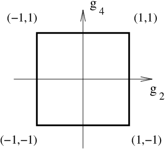
In our numerical calculations we varied the coupling constants $g_{2}$ and $g_{4}$ along the square with corners $(\pm 1,\pm 1)$ shown in Figure 2. The truncation level that we used is $n=8$, that corresponds to a Hamiltonian truncated to $1624$ conformal states. The finite volume spectra shown in Figures 4, 8, 9 and 10 are always plotted as functions of $mR$, where $m$ is the mass gap, whose value depends however on the region of the coupling constants which each figure refers to.

Precisely at $\eta_{+}=-\infty$, the model has a first order phase transition. This means that along the negative vertical axis the theory has three degenerate ground states $|0\rangle$, $|+\rangle$ and $|-\rangle$: the vacuum $|0\rangle$ is even under the spin reversal symmetry $Q$, while $|+\rangle$ and $|-\rangle$ are mapped into each other: $|-\rangle=Q|+\rangle$ (see Figure 3.a). Right at $\eta_{+}=-\infty$, the theory presents also an exact supersymmetry: the particle spectrum consists of four kinks $|K_{-0}\rangle$, $|K_{0-}\rangle$, $|K_{0+}\rangle$ and $|K_{+0}\rangle$ of equal mass. These kinks, that do not have bound states, provide an irreducible representation of supersymmetry and their exact S-matrix was obtained in [11]. The action of the spin reversal symmetry $Q$ on the kinks is given by $Q|K_{-0}\rangle=|K_{+0}\rangle$, $Q|K_{0-}\rangle=|K_{0+}\rangle$.

On a cylinder of circumference $R$, the three degenerate vacua give rise to three exponentially split energy lines, for the phenomenon of tunneling that occurs at a finite volume. With periodic boundary conditions, there are however no energy lines corresponding to the one-particle states of the kinks. Above the three exponentially degenerate lines of the ground states, one finds instead doublets of lines corresponding to the neutral kink-antikink configurations (see Figure 4). The proper counting of the states appearing in the finite volume with periodic boundary conditions is explained in Figure 3.b.

It is now important to understand what happens if we deform the theory away from this integrable situation, moving into the fourth quadrant by means of the perturbation $g_{2}\int\varepsilon(x)\mathrm{d}x$ ($g_{2}>0$). The drastic effect of this perturbation is to lift the degeneracy of the three vacua: in the perturbed theory, the central vacuum $|0\rangle$ becomes the true ground state of the theory, whereas the other two vacua $|\pm\rangle$ become metastable ground states, separated from $|0\rangle$ by a gap

$$\Delta E\sim g_{2}(\langle\Omega|\epsilon|\Omega\rangle-\langle 0|\epsilon|0\rangle)\ ,$$

(4.1)

where $|\Omega\rangle=|\pm\rangle$. As a consequence, we expect that the kinks of the unperturbed system will get confined as soon as we move away from $\eta_{+}=-\infty$ by switching on the coupling $g_{2}$ of the energy operator $\epsilon$. This can be directly seen by the FFPT, reported in Appendix C: the two-particle form factors on the kink states of the $\epsilon$ operator have in fact a pole at $\theta=\rmi\pi$ [23]. The linear confining potential between the constituents of the two pairs of neutral kink-antikink states $|K_{0-}K_{-0}\rangle$ and $|K_{0+}K_{+0}\rangle$ gives rise then to a dense sequence of bound states, with the number of bound states going to infinity as $g_{2}\to 0$ [7] (see Figure 5).

This analytic result is indeed confirmed by our numerical calculations. In particular, Figure 6 shows that the number of particles below the stability threshold increases to infinity as the first order transition line is approached (i.e. $\eta_{+}\to-\infty$). This scenario is similar to the one observed in the scaling region of the critical Ising model near the thermal axis once it is perturbed by a magnetic field [6] and it realizes the so-called McCoy-Wu scenario [22]. An important difference from the Ising model, however, is the $\mathbb{Z}_{2}$ symmetry of our model. At $\eta_{+}=-\infty$, the two-kink states $|K_{0-}K_{-0}\rangle$ and $|K_{0+}K_{+0}\rangle$ (the rapidities of the kinks are suppressed) are mapped into each other by spin reversal, so they form degenerate pairs (although in finite volume this degeneracy is lifted). The two-kink states $|K_{-0}K_{0-}\rangle$ and $|K_{+0}K_{0+}\rangle$ also form similar degenerate pairs, and so do the two-kink states $|K_{-0}K_{0+}\rangle$ and $|K_{+0}K_{0-}\rangle$. The degeneracy is lifted as soon as the perturbation is switched on; the arising bound states are singlets with definite parity. As the kinks do not have bound states at $\eta_{+}=-\infty$, all the bound states in the neighbourhood $g_{2}>0$ of the transition point arise from the free two-kink configurations mentioned above. Since the $|\pm\rangle$ vacua are lifted, the original two-particle states $|K_{-0}K_{0-}\rangle$, $|K_{+0}K_{0+}\rangle$, $|K_{-0}K_{0+}\rangle$, and $|K_{+0}K_{0-}\rangle$ of the continuum disappear entirely from the spectrum. In their place, there is a sequence of bound states $|B_{n}^{\pm}\rangle$, which arises from the even and odd superpositions of the $|K_{0-}K_{-0}\rangle$ and $|K_{0+}K_{+0}\rangle$ states:

$$|B_{n}^{\pm}\rangle\sim\frac{|K_{0-}K_{-0}\rangle\pm|K_{0+}K_{+0}\rangle}{\sqrt{2}}\ .$$

(4.2)

The superscript in $|B_{n}^{\pm}\rangle$ denotes parity, the subscript numbers the elements of the tower of bound states. As we mentioned, $|B_{n}^{+}\rangle$ and $|B_{n}^{-}\rangle$ are not degenerate. Due to the exactness of the $\mathbb{Z}_{2}$ symmetry the vacuum is expected to be even, and then the first state above it, i.e. the lowest one-particle state, is expected to be odd, and generally the parity is expected to alternate in the sequence of one-particle states.

The numerical data that we obtained by varying $\eta_{+}$ indeed confirm that in the high temperature phase the spin reversal symmetry is unbroken, there is a unique vacuum and the excitations are singlet scalar particles with alternating parity. The disappearance of the two-kink states $|K_{-0}K_{0-}\rangle$, $|K_{+0}K_{0+}\rangle$, $|K_{-0}K_{0+}\rangle$ and $|K_{+0}K_{0-}\rangle$ does not have a drastic effect on the numerical spectrum on the cylinder with periodic boundary conditions, since the $|K_{-0}K_{0+}\rangle$, and $|K_{+0}K_{0-}\rangle$ are filtered out and $|K_{-0}K_{0-}\rangle$ and $|K_{+0}K_{0+}\rangle$ are identified with $|K_{0-}K_{-0}\rangle$ and $|K_{0+}K_{+0}\rangle$ under these boundary conditions: what happens is that, energy lines that were previously asymptotic degenerate, now become separated by tiny gaps.

The doubly degenerate false vacuum can be seen in the $\eta_{+}<0$ domain in the TCSA spectra in the form of a linearly rising double line-like pattern (see Figure 9.a). The slope of the pattern, which equals to the gap $\Delta E$ between the false and true vacua, increases from $0$ as $\eta_{+}$ is increased, and finally the pattern disappears from the finite volume spectrum as $\eta_{+}$ approaches $0$. $\Delta E$ can be calculated by FFPT around the first order phase transition line. At $g_{4}=-1$ the exact result to first order in perturbation theory is

$$\frac{\Delta E}{g_{2}}=0.3076...=2\Lambda_{2}\times(2\pi)^{\frac{1-\Delta_{2}-\Delta_{4}}{1-\Delta_{4}}}\lambda_{4}^{\frac{\Delta_{2}}{1-\Delta_{4}}}\lambda_{2}\ ,$$

(4.3)

where

$$\Lambda_{2}=2.668319...$$

(4.4)

is the exact value of the vacuum expectation values of $\varepsilon$ given in [25, 26], and the factor next to $2\Lambda_{2}$ arises from various normalization factors used in the present paper and in [25, 26] (see Appendix B for more details on the calculation of $\Delta E$). On the other hand, by TCSA we obtain

$$\frac{\Delta E}{g_{2}}=0.29,$$

(4.5)

which is in reasonable agreement with the exact value.

Figure 6 shows the numerically calculated mass ratios $m_{i}/m_{1}$ ($m_{1}$ being the mass of the lightest particle) as functions of $\eta_{+}$. Truncation errors tend to increase for large absolute values of $\eta_{+}$, therefore the figure shows only a limited range around $\eta_{+}=0$. The masses $m_{1}$ and $m_{2}$ of the two lightest particles are also shown in Figure 7. The stability threshold, taking into account spin reversal symmetry, is $2m_{1}$ for even particles and $m_{1}+m_{2}$ for odd particles (if there are no even particles, then the threshold is $3m_{1}$).

Hence, increasing $\eta_{+}$, the number of stable excitations decreases. Around $\eta_{+}=0$, i.e. near to the positive horizontal axis, there are four stable excitations. However, precisely at $\eta_{+}=0$, the theory acquires three more stable particles, all of them above threshold. In order to understand the nature of the spectrum near to $\eta_{+}=0$, it is obviously more convenient to switch to the integrable formulation of the theory along the positive horizontal axis.

As we mentioned in the introduction, the $\eta=0$ line corresponds to an integrable model related to the Toda field theory based on the exceptional Lie algebra $E_{7}$. In the high temperature phase, this integrable model has a spectrum composed of seven scalar particles $A_{i}$, $i=1\dots 7$. Their masses $m_{i}$, $i=1\dots 7$ (see Table 1) and S-matrix amplitudes are known exactly [13, 14].

Note that $A_{1}$, $A_{3}$ and $A_{6}$ are odd under spin reversal symmetry while the other particles are even. Only the first four particles have a mass below the stability thresholds $2m_{1}$ and $m_{1}+m_{2}$. The higher three particles are nevertheless stable along this axis due to the integrability of the theory.

Moving away from the axis $\eta_{+}=0$, the expectation is that there exists a range of values of $\eta_{+}$ where the four lowest particles are still stable, whereas the higher three particles decay in all possible channels compatible with the symmetry of the perturbation. The perturbation that breaks the integrability of the theory at $\eta_{+}=0$ and plays the role of the operator $\Upsilon(x)$ in eqn (3.1) is the field $t$, which is even under the $\mathbb{Z}_{2}$ spin reversal symmetry. This implies certain selection rules in the decay processes. So, for instance, the particle $A_{5}$ can only decay in the channel

$$A_{5}\rightarrow A_{1}\,A_{1}\,,$$

(4.6)

even though the decay process $A_{5}\rightarrow A_{1}\,A_{2}$ would be permitted by kinematics. Similarly, it is easy to check that the other possible decay processes compatible with the selection rule are

	$\displaystyle A_{6}\rightarrow A_{1}\,A_{2}$
	$\displaystyle A_{7}\rightarrow A_{1}\,A_{1}$
	$\displaystyle A_{7}\rightarrow A_{2}\,A_{2}$		(4.7)
	$\displaystyle A_{7}\rightarrow A_{1}\,A_{3}$
	$\displaystyle A_{7}\rightarrow A_{2}\,A_{4}$
	$\displaystyle A_{7}\rightarrow A_{1}\,A_{1}\,A_{2}\,.$

The decay processes have a fingerprint in the finite volume spectra, namely the repulsion of the energy lines [6]. Observe, for instance, Figure 8.a: this refers to the lowest energy difference lines above the two-particle threshold (in the even sector only) on the integrable $E_{7}$ axis. One can see that there are several level crossings; in particular there is one around $mR\sim 12$ between the first and the second lines. The first line corresponds to the threshold state $|A_{1}A_{1}\rangle$, whereas the second line corresponds to the particle $|A_{5}\rangle$. When we switch on the $g_{4}$ perturbation, the crossing disappears, as it can clearly be seen in Figure 8.b. In particular, the repulsion of the first and second lines at $mR\sim 12$ corresponds to the decay $A_{5}\to A_{1}A_{1}$.

In principle, the widths $\Gamma^{k}_{ij}$ of the decays $A_{k}\to A_{i}A_{j}$ can be determined from the repulsion of energy lines by a method proposed in [28]. In this approach, which was called Breit-Wigner method in [28], $\Gamma$ is related to the two-particle phase shifts of the various two-particle levels $|A_{i}A_{j}\rangle$. In more detail, in order to measure $\Gamma$ one can use the formula

$$\Delta\delta={\rm min}\,\delta_{1}(E)-{\rm max}\,\delta_{2}(E)=4\sqrt{-\beta\Gamma}\ ,$$

(4.8)

where

$$\beta=\left.\frac{{\rm d}\delta_{0}}{{\rm d}E}\right|_{E=E_{k}}$$

(4.9)

should be negative, $E_{k}$ is the center of the resonance and $\delta_{0}(E)$ is defined by the integrable S-matrix as

$$\delta_{0}(E)=-\rmi{\rm\,ln\,}S(E)\ .$$

(4.10)

For the sake of clarity, we have suppressed the labels $i$, $j$, $k$ relative to the particles. The symbols $\delta_{1}(E)$, $\delta_{2}(E)$ in (4.8) refer to the phase shifts of two neighbouring two-particle levels $|A_{i}A_{j}\rangle$ and are given by

$$\delta_{a}(E)\,=\,-R(E)\,p_{a}(E),\qquad a=1,2\ ,$$

(4.11)

where $R$ is the circumference of the cylinder and $p_{a}(E)$ is the momentum, defined by the equation

$$E\,=\,\sqrt{p_{a}^{2}+m_{i}^{2}}+\sqrt{p_{a}^{2}+m_{j}^{2}}\ .$$

(4.12)

Hence, from the numerical determination of the energy levels we can measure $E(R)$ as a function of $R$; from this measurement, using (4.11), we can extract $\delta_{1}(E)$ and $\delta_{2}(E)$, and then (4.8) provides $\Gamma$.

Using the above consideration we have studied the decay processes

	$\displaystyle A_{5}\to A_{1}A_{1}$
	$\displaystyle A_{6}\to A_{1}A_{2}$

at $g_{2}=1$ and small $g_{4}$, finding the following numerical values for the decay rates

$$\Gamma^{5}_{11}\sim 2\cdot g_{4}^{2}\ ,\qquad\Gamma^{6}_{12}\sim 0.2\cdot g_{4}^{2}\ ,$$

(4.13)

and therefore the universal ratio

$$\frac{\Gamma^{6}_{12}}{\Gamma^{5}_{11}}\,\sim\,0.1\ .$$

(4.14)

This result shows that the decay of $A_{6}$ is considerably slower than the decay of $A_{5}$. Although the kinematical phase space factor $\Phi^{M}_{m_{i},m_{j}}$ generally tends to suppress the decay of heavier particles in $1+1$ dimensions [29], in the present case this effect is not sufficient, however, to justify the result above: in fact, the phase space estimate of the universal ratio (4.14) gives in this case

$$\frac{\Gamma^{6}_{12}}{\Gamma^{5}_{11}}\sim\frac{\Phi^{6}_{12}}{\Phi^{5}_{11}}\,=\,\sqrt{\frac{m_{5}^{2}(m_{5}^{2}-4m_{1}^{2})}{(m_{6}^{2}-(m_{1}-m_{2})^{2})(m_{6}^{2}-(m_{1}+m_{2})^{2})}}=0.783...\ .$$

(4.15)

Therefore the longer lifetime of $A_{6}$ has to be attributed to the dynamics of the model. We plan to analyze this aspect in a future publication.

Coming back to the stable particles of the spectrum, it is relatively easy to compute the correction to the masses of the two lowest particles once we move away from the $E_{7}$ integrable axis. This can be done by combining the FFPT and the TCSA, together with a cross-checking between the two methods. The first order mass correction of the particle $A_{i}$ moving away from the $\eta_{+}=0$ axis is given by

$$\delta m_{i}=\frac{g_{4}}{m_{i}}2\pi\lambda_{4}F^{t}_{ii}(\rmi\pi),$$

(4.16)

where $F^{t}_{ii}(\theta_{1}-\theta_{2})=\langle 0|t(0)|A_{i}(\theta_{1})A_{i}(\theta_{2})\rangle$ is the two-particle form factor of $t$. As a matter of fact, $F^{t}_{11}(\rmi\pi)$, $F^{t}_{22}(\rmi\pi)$, $F^{t}_{33}(\rmi\pi)$ and $F^{t}_{44}(\rmi\pi)$ can be directly extracted by TCSA (see Appendix B and [24, 26]). At $g_{2}=1$ we obtained

	$\displaystyle F^{t}_{11}(\rmi\pi)$	$\displaystyle=-\frac{1.28}{2\pi\lambda_{4}}\ ,\qquad F^{t}_{22}(\rmi\pi)$	$\displaystyle=-\frac{1.25}{2\pi\lambda_{4}}\ ,$		(4.17)
	$\displaystyle F^{t}_{33}(\rmi\pi)$	$\displaystyle=-\frac{2.03}{2\pi\lambda_{4}}\ ,\qquad F^{t}_{44}(\rmi\pi)$	$\displaystyle=-\frac{3.41}{2\pi\lambda_{4}}\ .$		(4.18)

Similarly, from TCSA we can also compute the absolute value of the one-particle form factors $F_{2}^{t}=\langle 0|t(0)|A_{2}(\theta)\rangle$ and $F_{4}^{t}=\langle 0|t(0)|A_{4}(\theta)\rangle$. The result is

$$|F_{2}^{t}|\,=\,\frac{0.35}{2\pi\lambda_{4}}\ ,\qquad|F_{4}^{t}|\,=\,\frac{0.26}{2\pi\lambda_{4}}\ .$$

(4.19)

As shown in the Appendix A, there is an exact relation between the two-particle form factors $F^{t}_{11}(i\pi)$ and $F^{t}_{22}(i\pi)$ and the one-particle form factors $F^{t}_{2}$ and $F^{t}_{4}$, expressed by

	$\displaystyle F_{11}^{t}(\rmi\pi)$	$\displaystyle=11.397\cdot F_{2}^{t}+10.3632\cdot F_{4}^{t}$			(4.20)
	$\displaystyle F_{22}^{t}(\rmi\pi)$	$\displaystyle=23.1056\cdot F_{2}^{t}+26.2404\cdot F_{4}^{t}\ .$			(4.21)

If we assume that $F_{2}^{t}<0$ and $F_{4}^{t}>0$, then (4.19), (4.20) and (4.21) yield

$$F^{t}_{11}(\rmi\pi)\,=\,\frac{-1.29}{2\pi\lambda_{4}}\ ,\qquad F^{t}_{22}(\rmi\pi)\,=\,\frac{-1.26}{2\pi\lambda_{4}}\ ,$$

(4.22)

which is in satisfactory agreement with (4.17).

With the above values, we can extract the universal ratios

	$\displaystyle\delta m_{2}/\delta m_{1}=0.76\ ,$
	$\displaystyle\delta m_{3}/\delta m_{1}=0.84\ ,$		(4.23)
	$\displaystyle\delta m_{4}/\delta m_{1}=1.35\ .$

In order to get another universal ratio, let us look at the first order correction to the vacuum energy density $\epsilon_{vac}$. By TCSA (see Appendix B) we obtain

$$\frac{\delta\epsilon_{vac}}{g_{4}}=0.11\ .$$

(4.24)

On the other hand, the exact value of this quantity is

$$\frac{\delta\epsilon_{vac}}{g_{4}}=0.1130...=\Lambda_{4}\times(2\pi)^{\frac{1-\Delta_{2}-\Delta_{4}}{1-\Delta_{2}}}\lambda_{2}^{\frac{\Delta_{4}}{1-\Delta_{2}}}\lambda_{4}\ ,$$

(4.25)

which is in good agreement with the above numerical result. $\Lambda_{4}=3.70708...$ is the vacuum expectation value of $t$ calculated in [25, 26] (the factor next to $\Lambda_{4}$ arises from various normalization factors used in the present paper and in [25, 26]). This allows us also to extract the universal ratio

$$\frac{\delta\epsilon_{vac}}{m_{1}\delta m_{1}}=-0.086\ .$$

(4.26)

After the analysis in the previous section we can now proceed to investigate the evolution of the spectrum in the first quadrant. First of all, note that the corrections to the two lowest masses have the same sign, which depends on the sign of $g_{4}$. We can use the above results for $\delta m_{1}$ and $\delta m_{2}$ to estimate the value of $\eta_{+}^{(2)}$ where the mass $m_{2}(\eta_{+})$ of the second particle reaches the threshold $2m_{1}(\eta_{+})$ of the lowest particle. This happens for a value of $\eta_{+}>0$ of the first quadrant, given by $\eta_{+}^{(2)}\simeq 1$: although this is higher than the value $\eta_{+}^{(2)}\simeq 0.7$ extracted from the numerical data shown in Figure 6, it is nevertheless a reasonable estimation of this quantity since the theoretical result was based on just first-order perturbation theory.

Besides the three higher particles $A_{5},A_{6},A_{7}$ that were stable only at $\eta_{+}=0$ and decay as soon as we move away from the horizontal axis, the TCSA analysis shows that the same pattern as was seen in the fourth quadrant also persists in the first quadrant: namely, increasing the value of $\eta_{+}$, the number of stable particles continues to decrease. The first particle that disappears into the threshold $2m_{1}(\eta_{+})$ is $A_{4}$ at the critical value $\eta_{+}^{(4)}$, which can be estimated from first-order perturbation theory to be $\eta_{+}^{(4)}\simeq 0.04$. This is followed by $A_{3}$ that disappears into its lowest threshold, given by ($m_{1}(\eta_{+})+m_{2}(\eta_{+}))$, at the critical value $\eta_{+}^{(3)}$, for which perturbation theory gives $\eta_{+}^{(3)}\simeq 0.62$. These theoretical results for $\eta_{+}^{(3)}$ and $\eta_{+}^{(4)}$ are in reasonably good agreement with the numerical data (Figure 6). An example of the finite volume spectra calculated numerically is shown in Figure 10.a at $\eta_{+}=0.3$, where the theory contains $3$ stable particles.

As just described, moving toward the positive vertical axis, there is a depletion of the number of stable particles, until there remains only one in the neighbourhood of $\eta_{+}=+\infty$. At the same time, notice that increasing $\eta_{+}$, the value of this lowest mass becomes also smaller⁴⁴ 4 This behavior is in agreement with the first-order correction (4.16) to $m_{1}$, that is negative for $g_{4}>0$.. The mass gap of the theory finally vanishes when $\eta_{+}=+\infty$, i.e. when we have reached the vertical axis.

During this evolution, however, there has also been a qualitative change of the spectrum: in fact, reaching the positive vertical axis the lowest excitation has turned into a fermion. This becomes evident by looking directly at the nature of the theory at $\eta_{+}=+\infty$ (notice that the positive vertical axis also corresponds to $\eta_{-}=+\infty$).

The analytic control of the theory in the vicinity of $\eta_{\pm}=+\infty$ is provided by the integrability of the model along the vertical axis, where the system is also supersymmetric. Along the positive vertical axis the supersymmetry is however spontaneously broken: the low-energy excitations are given in this case by the massless right and left mover Majorana fermions, which play the role of goldstino [10, 11, 12]. The factorized scattering theory was proposed in [11] and the basic form factors were calculated in [21]. The massless Majorana fermions are nothing else than those of the Ising model, connected to the TIM by the massless renormalization group flow that occurs along this line.

Breaking the integrability of the $\eta_{\pm}=\infty$ model by means of the operator $\Upsilon=\varepsilon$, the left and right moving excitations become adiabatically massive, as it can be directly observed in the TCSA data (see Figure 7). To compute the mass $m$ of the fermion generated by the perturbation, we need to employ in this case the massless FFPT [8]: at the lowest order, we have

$$m\simeq g_{2}\lim_{\theta_{RL}\to-\infty}F_{RL}^{\varepsilon}(\rmi\pi+\theta_{RL})\ ,$$

(4.27)

where the two-particle (right-left) form factor of the $\varepsilon$ operator is given by [21]

$$F^{\varepsilon}_{RL}(\theta)\,=\,\exp\left(\frac{\theta}{4}-\int_{0}^{\infty}\frac{\mathrm{d}t}{t}\frac{\sin^{2}\left(\frac{(\rmi\pi-\theta)t}{2\pi}\right)}{\sinh t\cosh\frac{t}{2}}\right)\ .$$

(4.28)

Using (4.27) and (4.28), one can easily check that $m$ is a finite quantity, positive for $g_{2}>0$ and negative for $g_{2}<0$. Note that, for a Majorana fermion, a negative value of the mass signals that we are in a low temperature phase, i.e. that the theory has two degenerate vacua. This is the topic of the next section.

At $\eta_{-}=-\infty$ the model is at the first order phase transition point, which was described in Section 4.1. As we move into the third quadrant by switching on the perturbation $g_{2}\int\varepsilon(x)\mathrm{d}x$ $(g_{2}<0)$, the degeneracy of the three vacua is lifted. In contrast with the fourth quadrant, the central vacuum $|0\rangle$ now becomes a metastable ground state, and the two other vacua $|\pm\rangle$ remain true ground states. The gap $\Delta E$ separating $|0\rangle$ from $|\pm\rangle$ at a given point is equal to the gap at the dual point in the fourth quadrant. The expected consequence of the lifting of the degeneracy of the vacua is again the confinement of the kinks of the unperturbed system, which is confirmed by the same FFPT argument as for the fourth quadrant. The linear confining potential between the kinks gives rise to a dense sequence of bound states. As in the fourth quadrant, the number of these bound states goes to infinity as $g_{2}\to 0$. In the third quadrant, however, the two-kink states $|K_{0-}K_{-0}\rangle$ and $|K_{0+}K_{+0}\rangle$ are those which disappear from the spectrum, and the bound states arise from the other two-kink states $|K_{-0}K_{0+}\rangle$, $|K_{+0}K_{0-}\rangle$, $|K_{-0}K_{0-}\rangle$ and $|K_{+0}K_{0+}\rangle$. Some of the bound states above are topologically charged, i.e. they are kinks, while others are neutral. The neutral particles arise from the neutral two-kink configurations:

$$|C^{n}\rangle_{+}\sim|K_{+0}K_{0+}\rangle,\qquad|C^{n}\rangle_{-}\sim|K_{-0}K_{0-}\rangle.$$

(5.2)

It is important to note that $|C^{n}\rangle_{+}$ and $|C^{n}\rangle_{-}$ are degenerate for any given $n$, due to the spontaneously broken $\mathbb{Z}_{2}$ symmetry, although their degeneracy is exponentially lifted in finite volume. The topologically charged particles arise from topologically charged two-kink states:

$$|\mathcal{D}^{n}_{-+}\rangle\sim|K_{-0}K_{0+}\rangle,\qquad|\mathcal{D}^{n}_{-+}\rangle\sim|K_{-0}K_{0+}\rangle,$$

(5.3)

where the subscripts $-+$ and $+-$ in $|\mathcal{D}^{n}_{-+}\rangle$ and $|\mathcal{D}^{n}_{+-}\rangle$ denote the vacua between which these kink configurations interpolate. $|\mathcal{D}^{n}_{-+}\rangle$ and $|\mathcal{D}^{n}_{+-}\rangle$ are mapped into each other by the spin reversal: $Q|\mathcal{D}^{n}_{-+}\rangle=|\mathcal{D}^{n}_{+-}\rangle$, therefore they have equal mass.

As we mentioned, under duality an even particle $|B_{n}^{+}\rangle$ in the high temperature phase corresponds to the neutral particles $|C^{n}\rangle_{\pm}$ of the same mass in the low temperature phase, and an odd particle $|B_{n}^{-}\rangle$ corresponds to a kink-antikink pair $|\mathcal{D}^{n}_{+-}\rangle$, $|\mathcal{D}^{n}_{-+}\rangle$ of the same mass.

The neutral particles $|C^{n}\rangle_{\pm}$ (more precisely, their even and odd superpositions) can indeed be seen in the TCSA spectra, whereas the kinks $|\mathcal{D}^{n}_{+-}\rangle$ and $|\mathcal{D}^{n}_{-+}\rangle$ are filtered out by the periodic boundary conditions. The neutral two-kink states constituted by $|\mathcal{D}^{n}_{+-}\rangle$ and $|\mathcal{D}^{n}_{-+}\rangle$ can nevertheless be observed in the numerical data. The disappearance of the original two-kink states $|K_{0-}K_{-0}\rangle$ and $|K_{0+}K_{+0}\rangle$ does not have drastic effect on the spectra with periodic boundary conditions for similar reasons as for the third quadrant.

The false vacuum with even parity can also be seen in the $\eta_{-}<0$ domain in the TCSA spectra in the form of a linearly rising line-like pattern (see Figure 9.b). The duality relates this metastable vacuum to the metastable vacua in the first quadrant.

The number of stable particles at any given point in the low temperature phase is equal to the number of particles in the dual point in the high temperature phase, and this number decreases as $\eta_{-}$ is increased. The number of stable particles around $\eta_{-}=0$ is $4$, however at $\eta_{-}=0$, i.e. on the negative horizontal axis, $3$ more particles become stable above threshold. These particles are related by duality to the three highest particles existing at $\eta_{+}=0$. In particular, there are two neutral particles $|C^{5}\rangle_{\pm}$, $|C^{7}\rangle_{\pm}$ of masses $m_{5}$ and $m_{7}$ (see Table 1) which correspond to the even particles $|A_{5}\rangle$, $|A_{7}\rangle$, and there is one kink-antikink pair $|\mathcal{D}^{6}_{+-}\rangle$, $|\mathcal{D}^{n}_{-+}\rangle$ of mass $m_{6}$ corresponding to the odd particle $|A_{6}\rangle$.

References

- [1] Belavin A, Polyakov A and Zamolodchikov A, 1984 Nucl. Phys. B 241 333; Friedan D, Qiu Z and Shenker S, 1984 Phys. Rev. Lett 52 1575
- [2] Friedan D, Qiu Z, Shenker S, 1985 Phys. Lett. B. 151 37
- [3] Goddard P, Kent A and Olive D I, 1986 Commun. Math. Phys. 103 105
- [4] Lukyanov S L and Fateev V A, 1989 Sov. J. Nucl. Phys. 49 925 [Yad. Phys. 49 (1989) 1491]
- [5] Lassig M, Mussardo G and Cardy J L, 1991 Nucl. Phys. B 348 591–618
- [6] Delfino G, Mussardo G and Simonetti P, 1996 Nucl. Phys. B 473 469
- [7] Delfino G and Mussardo G, 1995 Nucl. Phys. B 455 724 [hep-th/9507010]
- [8] Controzzi D and Mussardo G, 2005 Phys. Lett. B 617 133-139 [hep-th/0503018]
- [9] Mussardo G, 2007 JHEP 0708: 003 arXiv:0706.2546 [hep-th]
- [10] Zamolodchikov A B, in “Fields, strings and quantum gravity”, Proceedings of the Beijing Conference 1989, edited by Al.B. Zamolodchikov, p. 349. [Nucl. Phys. B 358 (1991) 497]
- [11] Zamolodchikov Al B, 1991 Nucl. Phys. B 358 524
- [12] Kastor D A, Martinec E J and Shenker S H, 1989 Nucl. Phys. B 316 590
- [13] Christe P and Mussardo G, 1990 Nucl. Phys. B 330 465
- [14] Fateev V A and Zamolodchikov A B, 1990 Int. J. Mod. Phys. A 5 1025
- [15] Zamolodchikov A B, 1986 Sov. J. Nucl. Phys. 44 529
- [16] Karowski M and Weisz P, 1978 Nucl. Phys. B 139 445
- [17] Smirnov F A, Form Factors in Completely Integrable Models of Quantum Field Theory (World Scientific) 1992.
- [18] Yurov V P and Zamolodchikov A B, 1990 Int. J. Mod. Phys. A 5 3221–3246
- [19] Klassen T R and Melzer E, 1992 Nucl. Phys. B 370 511–550
- [20] Fateev V A, 1994 Phys. Lett. B. 324 45
- [21] Delfino G, Mussardo G and Simonetti P, 1995 Phys. Rev. D 51 6620
- [22] McCoy B M and Wu T T, 1978 Phys. Rev. D 18 1259
- [23] Delfino G, 1999 Nucl. Phys. B 554 537–551 [hep-th/9903082]
- [24] Guida R and Magnoli N, 1997 Phys. Lett. B 411 127-133
- [25] Fateev V, Lukyanov S, Zamolodchikov A and Zamolodchikov A, 1998 Nucl. Phys. B 516 652-674
- [26] Fioravanti D, Mussardo G and Simon P, 2001 Phys. Rev. E 63 016103 [cond-mat/0008216]
- [27] Acerbi C, Mussardo G and Valleriani A, 1996 Int. J. Mod. Phys. A 11 5327–5364 [hep-th/9601113]
- [28] Pozsgay B and Takács G, 2006 Nucl. Phys. B 748 485 [hep-th/0604022]
- [29] Delfino G, Grinza P and Mussardo G, 2006 Nucl. Phys. B 737 291 [hep-th/0507133]
- [30] Tóth G Zs, 2004 J. Phys. A 37 9631–9650 [hep-th/0406139]
- [31] Tóth G Zs, “Investigations in two-dimensional quantum field theory by the bootstrap and TCSA methods”, PhD thesis, Eötvös University, Budapest, 2006, arXiv:0707.0015[hep-th]