On the statistical significance of temporal firing patterns in multi-neuronal spike trains
Abstract
Repeated occurrences of serial firing sequences of a group of neurons with fixed time delays between neurons are observed in many experiments involving simultaneous recordings from multiple neurons. Such temporal patterns are potentially indicative of underlying microcircuits and it is important to know when a repeatedly occurring pattern is statistically significant. These sequences are typically identified through correlation counts, such as in the two-tape algorithm of Abeles and Gerstein [1]. In this paper we present a method for deciding on the significance of such correlations by characterizing the influence of one neuron on another in terms of conditional probabilities and specifying our null hypothesis in terms of a bound on the conditional probabilities. This method of testing significance of correlation counts is more general than the currently available methods since under our null hypothesis we do not assume that the spiking processes of different neurons are independent. The structure of our null hypothesis also allows us to rank order the detected patterns in terms of the strength of interaction among the neurons constituting the pattern. We demonstrate our method of assessing significance on simulated spike trains involving inhomogeneous Poisson processes with strong interactions, where the correlation counts are obtained using the two-tape algorithm [1].
1 Introduction
Detection of temporal firing patterns among groups of neurons is an important task in neuroscience as such patterns may be indicative of functional cell assemblies or microcircuits present in the underlying neural tissue [4, 12]. Analysis methods such as the two-tape algorithm of Abeles and Gerstein [1, 2] have been developed to discover repeating occurrences of precise firing sequences in simultaneous recordings from multiple neurons. The two-tape algorithm has been used to assess precisely timed activity patterns in vivo [10], in slices in vitro [8], and recently in cultures of dissociated cortical neurons [14]. The two-tape algorithm, as well as alternative methods for identifying spike coincidences such as the unitary event detection algorithm of Grun [6], determines statistical significance of the discovered patterns under a null hypothesis of independence among the neurons [3]. In this paper, we present a significance test that allows “weak interactions” to be included in the null hypothesis by characterizing the strength of influence among neurons in terms of a conditional probability, which is a very natural way to think about synaptic interactions between neurons).
Let us write a 3-neuron pattern as , denoting a firing sequence where is followed by after a delay of and is followed by after a delay of . Most methods count the occurrences of this pattern by essentially finding correlations among time shifted spike trains from , , and . There are also many methods to determine the statistical significance of these patterns based on how many times they occur (see [5] and references therein). To assess whether a given number of repetitions of the pattern is significant, one generally employs a null hypothesis that assumes that all neurons spike as (possibly inhomogeneous) Poisson processes and that different neurons are independent. Based on this one can analytically calculate a bound on the number of repetitions required to make a pattern significant in the sense of being able to reject the null hypothesis at a given level of confidence. There are also methods to assess significance through empirical means [7]. In these methods, one generates many surrogate data streams of spike trains by systematically perturbing the spikes in the original data and then assesses significance of a pattern by noting the difference in counts (or in any other statistic derived from such correlation counts) for these patterns in the original data and in the surrogate streams. In these “jitter” methods, often the implicit null hypothesis is also independence.
When a sequential firing pattern like is declared as significant by any of these methods, the underlying idea is that we can conclude that , , and influence each other in a sequential fashion because we are able to reject the null hypothesis of independence. However, these methods do not say anything about the “strength of influence” among neurons , , and . We present a method for analyzing statistical significance of sequential firing patterns that also allows rank ordering of significant patterns in terms of the strength of influence among participating neurons. Thus our method extends the currently available techniques of significance analysis.
We represent the strength of influence of on by the conditional probability that would fire after the delay given that has fired now, which we denote as . Our null hypothesis is then stated in terms of a bound on all such pairwise conditional probabilities and we develop a statistical significance test for rejecting the null hypothesis. By changing the parameter of the null hypothesis (which is the bound on the conditional probability), we are able to see which patterns are significant at different levels of strength of influence.
Another interesting consequence of our approach is that since the null hypothesis is stated in terms of bounds on pairwise conditional probabilities, our null hypothesis includes not only all models of independent neurons but also some models of dependent or interacting neurons. This is more general than what is available in current methods. Intuitively, declaring a pattern like as significant should mean that we can conclude that there are “strong” causative connections from to and from to with the indicated delays. Hence rejecting a null hypothesis that includes not only independent neuron models but also models of neurons that are “weakly” dependent is more appropriate. Our method specifies these “weak interactions” in terms of bounds on conditional probabilities.
The rest of the paper is organized as follows. In Section 2 we present our significance test. We first explain our composite null hypothesis and then develop a test of significance. In Section 3 we demonstrate the effectiveness of the method through computer simulations. Spike trains are generated by a network of neurons modeled as interdependent inhomogeneous Poisson processes. We show that our method rank orders significant patterns. Surprisingly, it is also quite effective in situations where some of the assumptions of our theoretical analysis are not valid. We conclude the paper in Section 4 with potential extensions and a discussion of strengths and weaknesses.
2 Methods
Correlation Count
For simplicity of exposition, we first explain the method for a sequential firing pattern of only two neurons. Consider a pattern . Suppose we find the number of repetitions of this pattern in the data using simple correlation as follows. Let denote all time instants at which there is a spike from any neuron in the data. Let
| (1) |
where for any neuron , if there is a spike from at time and zero otherwise. Note that is simply a correlation integral which counts the number of spikes from that are followed by with a delay of exactly units, and hence counts the number of repetitions of our pattern. If we want to allow for some small random variations in the delay we can define the indicator variable to take value 1 if there is a spike in a time interval of length centered around . (For example, we can take to be the time resolution in our measurements). From now on we assume that delays are always over some such small intervals.
There are many methods to calculate correlation counts, for example the two-tape algorithm of Gerstein and Abeles [1] and some of its recent variations [17]. Most current methods for detecting serial firing patterns rely on such correlations. Since the focus of this paper is on statistical significance (and not on computational efficiency), we simply assume that one can calculate such counts for pairs of neurons and for various delays of interest. The question then, is “how large should the count be to conclude that the pattern represents a “strong” influence of on ?”
Since we want to address this question in a classical hypothesis testing framework, we need to choose a null hypothesis that includes as many models as possible of interdependent neurons without any “strong” influences between pairs of neurons. Then, if we can calculate (or bound) the probability under the null hypothesis that is above a threshold, we get a test of statistical significance. As stated earlier, we want the null hypothesis to contain a parameter to denote the strength of influence so that we can rank order all significant patterns.
Strength of influence as conditional probability11 1 See [16] for the original formalism of using conditional probability as a measure of interaction strength and deriving bounds on counts
We propose that the strength of influence between any pair of neurons can be characterized in terms of a conditional probability. Let denote the conditional probability that will fire at time (or more precisely, in a time interval ) given that has fired at time zero. If, for example, there is a strong excitatory connection from to , this probability would be large. If, on the other hand, and are independent then would be the same as the unconditional probability of firing in an interval of length . (For example, if we take that and the average firing rate of is , then this unconditional probability would be about 0.02). We note here that this conditional probability is well defined even if the two neurons are not directly connected through a single synapse. If the pair is directly connected, then can be a typical mono-synaptic delay; otherwise can be a multiple of the mono-synaptic delay. In either case, our task is to find whether a pattern with a specific value for is significant.
This conditional probability is a good scale on which to say whether the influence of on is “strong”. Our main assumption here is that this conditional probability is not time dependent. That is, the probability that fires in an interval given that has fired at is the same for all for the time period of observations that we are analyzing. Some recent analysis of spike trains from neural cultures [9] suggests that such an assumption is justified. Note that this assumption does not require the firing rates of neurons to not be time-varying. As a matter of fact, one of the main mechanisms by which this conditional probability is realized is by having a spike from affect the rate of firing by for a short duration of time. Thus, the neurons would have time-varying firing rates even when the conditional probability is not time-varying. Our assumption is only that every time spikes, it has the same chance of eliciting a spike from after a delay of , i.e. there are no appreciable changes in synaptic efficacies during the period in which the data is gathered.
When analyzing the significance of repeating serial patterns, what we are interested in is hypothesizing causative chains. Hence the strength of a pattern should be related to the propensity that a spike from has on eliciting a spike from , which can be conveniently represented by the conditional probability of spiking given that has spiked. In all serial firing patterns of interest, the constancy of delays in multiple repititions are important. Hence we defined the conditional probability with respect to a specified delay. Capturing influences among neurons through this conditional probability allows us to formulate an interesting compound null hypothesis in terms of a bound on these probabilities.
Compound null hypothesis
Now we propose the following compound null hypothesis. Any model of interacting neurons is in our null hypothesis if it satisfies: for all neurons and a set of specified delays , where is a user-chosen constant. The exact mechanism by which a spike output by affects the spiking of is immaterial here. Whatever be the mechanism, if the resulting conditional probability is less than then that model would be included. Thus our compound null hypothesis includes many models of interdependent neurons where whether or not a neuron spikes can depend on actual spikes of other neurons (unless we choose to be very small). The idea is that we choose an based on how strong we want the influences to be before we agree to say there is a causative influence of on . For example, as given earlier, with , and an average rate of firing of , the conditional probability is 0.02 if the neurons are independent. So, if we choose , it means that we agree to call an influence strong if the conditional probability is twenty times what you would see if the neurons were independent. More importantly, if we have a test of significance for this null hypothesis, then by varying we can rank order different significant patterns in terms of the strength of influence.
Significance Test
To get a test for statistical significance we need to calculate a bound on the probability that, under this null hypothesis, the count is above a given threshold. For this, consider the following stochastic model. Suppose is the total time duration of the data and let the random variable denote the total number of spikes by neuron during this time. Define
| (2) |
where are independent and identically distributed 0-1 random variables with
| (3) |
If we take , it is easy to see that is a random variable equivalent to since every time there is a spike from , with probability a spike from would follow with the appropriate delay. Also, per our assumption, every time spikes a spike from with the appropriate delay occurs with the same probability regardless of ’s spike history. This implies that the in the definition of can be assumed to be independent and identically distributed.
Now we assume that the spiking of is Poisson. (Note that we are not assuming that spiking by is Poisson and, more importantly, as per our null model the spiking process of is not independent of that of .)22 2 Indeed when spiking by is Poisson, the spiking of would not be Poisson if there is sufficient influence of on . Also, in Section 3 we show empirically that our hypothesis testing method is effective even in cases when is not Poisson. Then the random variable is such that we are accumulating a random variable every time an event of a Poisson process happens. This implies that, since the are 0-1 random variables, is also a Poisson random variable [15, Ch.2.5].33 3 An equivalent way of looking at this is to consider the Poisson process of spikes from and suppose that we classify each spike as type-Y with probability and as type-N with probability . Then it can be shown that the sequence of type-Y spikes (and also the type-N spikes) would constitute a Poisson process. Here, the classification of each spike is dependent on whether or not there is a spike from after the appropriate delay and is independent of everything else. The mean and variance of are given by [15, Ch.2.5]
| (4) |
Let the rate of the Poisson process for be . Then, . Since, , is a Poisson random variable with expectation (and variance) .
Computing the threshold
Let be a Poisson random variable with mean . Suppose the allowed Type I error in our hypothesis test is . Let be the smallest number satisfying
| (5) |
Given and , we can calculate the needed to satisfy the above using the Poisson distribution. For a Poisson random variable, the probability on the LHS of Eq. (5) is monotonically increasing with as long as . We know that is Poisson with mean . Under our null hypothesis, we have . Hence, if we take and calculate the needed to satisfy Eq. (5), then we have, under our null hypothesis,
| (6) |
Since, as discussed earlier, the random variable represents the count , the above is the threshold on the count to reject our null hypothesis and hence conclude that the pattern found is significant.
The test of statistical significance is as follows. Let be the bound on conditional probability that we chose for our null hypothesis. Let be the allowed Type I error. Let be the rate of firing for the first neuron in the pattern. Set . Using the cumulative distribution of a Poisson random variable with parameter , we calculate the needed to satisfy Eq. (5). This is the threshold on the count of the pattern for us to be able to reject the null hypothesis and declare the pattern to be significant.
To calculate this threshold, we need . This is easily estimated from the data as the average rate of firing for neuron . A simple parametric study shows that the threshold is well-behaved (see Fig. 1).

Extending to longer patterns
Here we explain how the signficance test can be extended to patterns involving more than two neurons. Suppose we are considering the pattern . We assume we get the count of by taking 3-point correlations.44 4 In general, taking -point correlations like this for all possible -tuples of patterns is computationally expensive. For this reason, such correlation counts are obtained only for patterns of length 3 or 4 in most cases. Here we are only explaining how our test can be extended to assess significance of longer patterns provided we can get such correlation counts. As before we define as a sum of 0-1 random variables . Now, we want to be 1 if the spike by is first followed by and then by with the indicated delays. Hence we take to be .55 5 This calculation for is correct if all influence of on comes only through . This is a reasonable assumption if we want significant patterns to represent a chain of triggering events. In such a case, would be same as . Even if there are other paths for to influence , this value of would represent a lower bound on the probability of the pattern occurring at any spike from . Hence, with this , would be less than and hence the threshold on the count calculated using this would be sufficient in a hypothesis testing framework. Under the null hypothesis, each of these conditional probabilities are less than . Hence, if we calculate the as needed in Eq. (5) with , then we get the needed threshold on the counts for this pattern. Now the method can easily be generalized to a pattern involving neurons. Let the first neuron in the pattern be . Then we calculate the threshold needed using Eq. (5) with .
The main point of the above analysis is that if the first neuron in a chain is Poisson then the counts of the pattern would be Poisson even if the other neurons in the chain are not Poisson. As a matter of fact, when the relevant conditional probabilities are high, the other neurons would not be Poisson. It was observed earlier [2] that the correlation counts can be assumed to be Poisson even when the neurons have time-varying rates and hence are not strictly Poisson (but may be inhomogenous Poisson). The analysis presented here can be viewed as a theoretical justification for this observation.
3 Results
Spike train simulator
In this section, we present results from computer simulations to demonstrate the effectiveness of our method. We used a simulator for generating spike data from a network of 25 interconnected neurons labeled through as shown in Fig. 2. There were four chains, each four neurons in length, with strong connections in the network (G-M-R-D, I-S-C-E, W-O-L-V, and P-A-T-K). The spiking of each neuron was an inhomogeneous Poisson process whose background firing rate of was modulated at time intervals of based on input received from neurons to which it was connected. Each synapse interconnecting neurons was characterized by a delay which was an integral multiple of and a strength in terms of a conditional probability. Using the notation from Section 2, the connections in the four chains were specified as follows (delays in ):
So among the four chains, the conditional probabilites ranged from 0.2 to 0.8 (with G-M-R-D being the weakest and P-A-T-K being the strongest) and the synaptic delays were between 2 and 5 . In some simulations the network also had many other interconnections in addition to the chains, where we connected each neuron to 25% of all the other neurons randomly. As stated earlier, with a average firing rate the unconditional probability of a neuron firing in is about 0.02. Hence we chose the strength (again in terms of conditional probabilities) of these random connections as uniformly distributed over the range , which is a factor of 2 on either side of the case of independence. Note that this means that the firing rate of a neuron (under the influence of random synapses) varies over the range of to where is the nominal background firing rate. The synaptic delays for the random connections were uniformly distributed between 2 and 5 . All neurons also had a refractory period of . Further details on the simulator can be found in Appendix B.
First neuron and pattern characteristics
We conducted simulations that verified the result derived in Section 2 that the occurrences of a pattern are Poisson-distributed when the first neuron in the pattern spikes according to a Poisson process. To do this we simulated the 25-neuron network shown in Fig. 2 for 100 seconds without any random connections. Since the only connections among neurons were the four chains (G-M-R-D, I-S-C-E, W-O-L-V, P-A-T-K), the spiking of the first neuron in each pattern (, , , ) should approximately follow a Poisson process. (Even here the spiking of the first neurons are not exactly Poisson-distributed since they have a refractory period of 1 ms. However, since this refractory period is small compared to the interspike intervals when firing at , the deviations from the Poisson firing due to the refractory period are small). We repeated the simulation 5,000 times obtaining the counts of and the counts of the pattern W-O-L-V. In Fig. 3 we show the histogram of these counts compared to a Poisson distribution with the rate parameter set as the sample mean for each count. The variance-to-mean ratio, or the Fano factor, for the count of is 0.97. Since the Fano factor of a Poisson random variable is 1 this indicated that the first neuron was approximately Poisson, and indeed a goodness-of-fit test failed to reject a null hypothesis of Poisson (P-value>0.05, test performed following the guidelines in [11]). The theory developed in Section 2 tells us that when the first neuron in a pattern is approximately Poisson the count of the pattern will also be approximately Poisson, and our empirical results confirmed this (W-O-L-V Fano factor 1.01, goodness-of-fit test P-value>0.05). Then we repeated the simulations this time allowing random connections between all neurons with 25% connectivity. We can see in Fig. 4 that when there are random connections in the network the first neuron in the pattern () and the pattern itself (W-O-L-V) are no longer approximately Poisson-distributed (Fano factor 2.66 and 1.51 for and W-O-L-V respectively). The goodness-of-fit test rejects the null hypothesis that these counts are Poisson (: P-value<0.01, W-O-L-V: P-value<0.01). Although the theory behind our significance thresholds assumes the first neuron spikes according to a Poisson process, we will now demonstrate empirically that even when the first neuron is not Poisson-distributed (due to random connections present in the network) we are still able to rank order the relative strength of patterns effectively using our significance thresholds.


Rank ordering of signficant patterns
Even when the pattern counts are not Poisson-distributed (as for the simulations shown in Fig. 4), we are still able to rank order the relative strengths of the patterns as shown in Fig. 5. We also see that the line showing the threshold count corresponding to is able to distinguish the counts of pattern G-M-R-D from the “maximum” of random 4-neuron pattern counts not involving any of the neurons in the four chains.

Data requirements
To determine how much data is required to rank order we simulated the network with random connections to all neurons (again with 25% connectivity) for various lengths of time, and for each data length compared the counts of the patterns to the thresholds corresponding to values which are 0.1 greater than and 0.1 less than the known connection strength of the chain producing the pattern. We found that the amount of data needed to achieve the desired resolution depends on the chain strength. We can see from Fig. 6 that for pattern G-M-R-D (strength 0.2) around 60 seconds of data is sufficient, while for patterns I-S-C-E, W-O-L-V, and P-A-T-K (strengths 0.4, 0.6, and 0.8) we need as little as 15 to 25 seconds of data. The data requirements are also dependent on firing rate, and with we find that 300 seconds of data is sufficient for the weakest pattern (G-M-R-D). We then used this firing rate and data length to demonstrate how our techniques can enhance the significance analysis of counts obtained using the two-tape algorithm of [1].

Enhanced significance analysis of two-tape algorithm counts
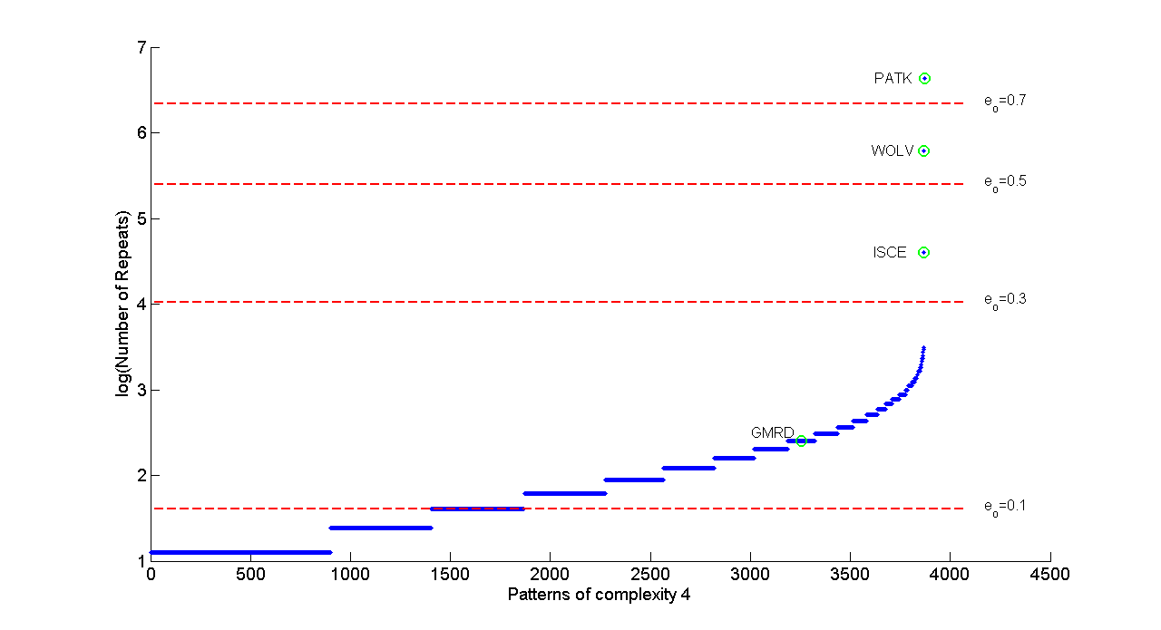
Abeles and Gerstein [1] provide a formula for calculating the expected number of patterns of a particular description that will occur times in data of length if the neurons spike according to independent Poisson processes. Based on this formula, if we had 25 independent spike trains and 300 seconds of data we would expect to find 3.86 patterns of complexity (length) four that repeat at least twice (with , , and the total time span between the spikes of the first and fourth neuron constrained to be or less). When we ran a simulation with these parameters and then mined the data with the two-tape algorithm we found six 4-neuron patterns that repeated twice or more and satisfied the temporal constraint. Again following [1], we calculated that this is not a statistically significant excess of patterns for a Poisson random variable with a mean of 3.86 (P-value>0.05). However if it had been, since it is a small number of patterns each pattern could be investigated further by the experimenter to determine which particular patterns out of the six are actually of interest. On the other hand, if the number of patterns found is large (and statistically significant) it is not practical to designate all patterns of that description as candidates for further investigation. To illustrate this, we repeated the simulation but instead of having independent neurons we had chains of connected neurons as shown in Fig. 2, as well as random connections between all neurons with 25% connectivity as described previously. This time when we mined with the two-tape algorithm we found 3,870 4-neuron patterns that repeated at least twice. Here we need some additional criteria to select which of these individual patterns are most likely to be significant and the best candidates for further analysis. Abeles and Gerstein [1] remarked that this selection process is very important, and called for future research to be conducted in this area to devise selection methods beyond their suggested strategy of repeating their analysis procedure for different subgroupings of the patterns (with the hopes of finding a smaller group of patterns that is significant which can then be investigated further to find the individual patterns responsible). Our framework of a compound null hypothesis based on conditional probabilities can be very useful as the selection criteria. By having different values for in the null hypothesis, we can ask what patterns are significant at what value of and thus rank order patterns according to their relative strength. We demonstrate this in Fig. 7 as our thresholds at various are able to separate the three strongest patterns (I-S-C-E, W-O-L-V, and P-A-T-K) from the rest based on the counts obtained using the two-tape algorithm. We also see that when mining with a threshold of there are a considerable number of false positives (i.e. there are other 4-neuron patterns that are more frequent than G-M-R-D, our weakest pattern). This is due to subpatterns (e.g. P-A-T) of the stronger patterns being very frequent, and as a consequence 4-neuron patterns such as P-A-T-X occur frequently even if there is no strong connection between T and X. Future work will address this issue.
4 Discussion
In this paper we proposed a method of assessing significance of serial firing patterns using correlation counts as the statistic. There are two attractive features of this method. First, we can rank order significant patterns in terms of their relative “strength”. For this we represent the strength of influence of on by the conditional probability that fires after a prescribed delay following . We state our composite null hypothesis in terms of a parameter which is an upper bound on all such pairwise conditional probabilities. This allows us to rank order significant patterns in terms the value of at which the pattern (which has a given number of repetitions) is no longer significant. The second interesting feature of the method follows from this structure of our composite null hypothesis. Since we now include many models of interdependent neurons (as long as all the relevant conditional probabilities are less than ), rejecting such a null hypothesis is intuitively more satisfying. When we declare a pattern such as as significant, we can conclude that a spike by has a “strong” influence in eliciting a spike from with delay and a spike from after a further delay of . Here “strong” would denote that the relevant conditional probability is greater than . Thus, our idea of casting the null hypothesis in terms of a bound on conditional probabilities allows for a richer level of analysis.
Computational considerations
We have given a simple test of statistical significance for deciding whether or not to reject the null (under a given confidence level) based on the counts calculated through simple multi-point correlations. As said earlier, the motivation is that such correlations are what are presently used for detecting such patterns.
At this point one may wonder whether there is any need for the test of significance that we presented, given that we formulate our null hypothesis in terms of conditional probabilities. The correlations counts as defined here would directly lead to an estimate of the conditional probability, . Hence, one can estimate the conditional probability and check whether it is less than . While it is true that we can directly get an estimate of the conditional probability, to get the required confidence intervals on the estimate, we once again need to use similar kind of assumptions as here and hence, theoretically, the testing procedure is not irrelevant. But there are other reasons why this approach is better than estimating all conditional probabilities.
First, our test will directly give the threshold needed for the count, given any pattern. Thus, we need not actually obtain the true correlation count which is required if we want to estimate the conditional probability. We only need to ascertain whether a pattern occurs more than some number of times. Many of the algorithms for detecting patterns use the correlations in this way and it leads to better computational efficiency.
There is a second and more interesting reason why our approach could be beneficial. In general, obtaining correlation counts or ascertaining whether a pattern occurs a given number of times is computationally intensive. If we want to look for long patterns, the number of candidate patterns increases exponentially and, furthermore, the multi-point correlation is difficult to compute. However, there may be other more appealing ways to count what may be called the frequency of a pattern. The correlation count we considered here counts all occurrences of the relevant pattern. Suppose we want to count only those occurrences such that the time span of one occurrence does not overlap with that of any other occurrence. Let us call such occurrences non-overlapped occurrences of the pattern. (This means, e.g., if the spike sequence is , then we count only one occurrence rather than two). There are very efficient algorithms based on data mining techniques for obtaining all patterns whose counts in terms of maximum possible number of non-overlapped occurrences are above a threshold [13]. These algorithms are also computationally efficient in discovering very long patterns involving more than ten neurons [13]. It appears possible to extend this type of statistical significance analysis to such counts also. Also, even when finding correlations, it is possible to tackle the combinatorial explosion in candidates (when we are looking for long patterns) by using similar data mining methods if we can put a bound on the count and decide that we are interested in only those patterns above this count. We will be addressing these issues in our future work. It is in terms of such generality that the approach presented here is interesting.
Strengths and weaknesses of the method
The strength of the approach is that we can accommodate dependence between neurons and conclude that some pattern is significant only if it represents strong influences among the set of neurons. Since this strength of influence is controlled by a parameter in the null hypothesis, we can rank order different significant patterns by varying this parameter.
However, the weakness of the specific test proposed here is that we need to assume that the first neuron in the chain is Poisson. The assumption was needed to conclude that the pattern counts would be Poisson. In most of the currently available methods, one also assumes Poisson processes in the null hypothesis. In general, if the variations in the rate of firing of a neuron are small (which would be the case if all synapses into the neuron are very weak) then the Poisson assumption is likely to be a good approximation. Thus, the assumption is not restrictive if we know that some neuron is necessarily the first in a chain. However, it is not always possible to have such knowledge. In spite of the assumption of Poissonness of the first neuron, we feel that the approach presented here is interesting and useful.
Summary
In this paper we suggested an analytical method to assess the statistical significance of sequential firing patterns with constant delays between successive neurons. The main methods of detecting such patterns depend on multi-point correlations. Our method can be used to find thresholds on such correlation counts for deciding on the significance of the patterns. Our main motivation is to have a method that can rank order significant patterns in terms of the strength of influence among the neurons constituting the pattern. For this we suggested that the influence of on can be denoted in terms of the conditional probability of firing after a prescribed delay given that has fired. Our compound null hypothesis is then stated in terms of an upper bound on all such pairwise conditional probabilities. This upper bound is a parameter of the null hypothesis and by varying it we can compare different significant patterns in terms of the strength they represent. This feature is very novel in relation to the current methods of significance analysis. Another important consequence of our approach is that the null hypothesis now admits many models of interdependent neurons also in addition to the usual case of independence. Hence our approach to significance analysis is more general.
Through extensive simulation experiments we demonstrated the effectiveness of the method. The method is seen to work well and is seen to be able to rank order different patterns in terms of their strengths even when our assumption in the theoretical analysis, namely that the first neuron in the chain is Poisson, is not valid.
The method presented can assess significance of sequential firing patterns only when the underlying influences are excitatory. This is because the significance test is stated in terms of a lower bound on the correlation count. Using a similar null hypothesis where we assume that the conditional probability is much smaller than the case under independence, it may be possible to find how low the correlation count should be for us to conclude that there are significant inhibitory influences. This needs further investigation.
As we have pointed out there are some weaknesses in the approach. One is the assumption that the first neuron in the sequence is Poisson. The other is the computational problems involved in finding correlation counts when one wants to detect interactions among a large group of neurons. There are some efficient algorithms based on data mining techniques which find somewhat different counts but are computationally very efficient for discovering patterns involving large numbers of neurons [13]. We will be addressing the issue of extending the analysis presented here to such counts in our future work.
5 Appendix A
| Symbol | Meaning |
|---|---|
| neurons | |
| delay between neurons | |
| time resolution of measurement / update rate of simulator | |
| correlation integral (# of spikes of followed by with a delay of ) | |
| indicator variable for a spike in a time interval of centered around | |
| conditional probability that will fire in a time interval given that has fired at time 0 | |
| user chosen bound on conditional probability for null hypothesis () | |
| total time duration of data | |
| random variable for # of spikes by in data | |
| random variable representing correlation integral | |
| independent and identically distributed 0-1 random variables | |
| probability that | |
| rate of Poisson process for spiking of | |
| expectation of random variable | |
| Poisson random variable with mean | |
| Type I error in null hypothesis | |
| significance threshold (smallest number satisfying ) | |
| number of neurons in chain or pattern |
6 Appendix B
Simulation model
Here we describe the simulator used for generating spike data from a network of interconnected neurons. The spiking of each neuron is an inhomogeneous Poisson process whose rate of firing is updated at time intervals of . The neurons are interconnected by synapses and each synapse is characterized by a delay (which is in integral multiples of ) and a weight which is a real number. All neurons also have a refractory period. The rate of the Poisson process is varied with time as follows:
| (7) |
where is the firing rate of neuron at time , and are two parameters. is the total input into neuron at time and it is given by
| (8) |
where is the output of neuron (as seen by the neuron) at time and is the weight of synapse from to neuron. is taken to be the number of spikes by the neuron in the time interval where represents the synaptic delay (in units of ) for the synapse from to .
We build the network in the following manner. The parameter is chosen based on the dynamic range of firing rates that we need to span. The parameter is determined by specifying the background spiking rate. This is the firing rate of the neuron under zero input. (We normally keep the same background firing rate for all neurons). Specifying this rate fixes by using (7). The network has many random interconnections with low weight values and a few strong interconnections with large weight values. For the random connections we connect each neuron to some percentage of all the other neurons randomly. The weight values for these random connections are uniformly distributed over a suitable range. We specify all weights in terms of the conditional probabilities they represent. Given a conditional probability, we first calculate the needed instantaneous firing rate so that probability of at least one spike in the interval is equal to the specified conditional probability. Then using (7) and (8) we calculate the value of needed so that the receiving neuron () reaches this instantaneous rate given that the sending neuron () spikes once in the appropriate interval and assuming that input into the receiving neurons from all other neurons is zero. In our simulations, we specify the range of random weight values as well as the values of strong weights in terms of the equivalent conditional probabilities.
We then generate a spike train by simulating all the inhomogeneous Poisson processes where rates are updated every time instants. We also have a fixed refractory period for all neurons, so that once a neuron is fired we will not let it fire until the refractory period is over.
We note here that the background firing rate as well as the effective conditional probabilities in our system would have some small random variations. As said above, we fix so that on zero input the neuron would have the background firing rate. However, all neurons would have synapses with randomly selected other neurons and the weights of these synapses are also random. Hence, even in the absence of any strong connections, the firing rates of different neurons keep fluctuating around the background rate that is specified. Since we choose random weights from a zero mean distribution, in an expected sense we can assume the input into a neuron to be zero and hence the average rate of spiking would be the background rate specified. We also note that the way we calculate the effective weight for a given conditional probability is also approximate and we chose it for simplicity. If we specify a conditional probability for the connection from to , then, the method stated earlier fixes the weight of connection so that the probability of firing at least once in an appropriate interval given that has fired is equal to this conditional probability when all other input into is zero. But since would be getting small random input from other neurons also, the effective conditional probability would also be fluctuating around the nominal value specified. Further, even if the random weights have zero mean, the fluctuations in the conditional probability may not have zero mean due to the nonlinear sigmoidal relationship in (7). The nominal conditional probability value determines where we operate on this sigmoid curve and that determines the bias in the excursions in conditional probability for equal fluctuations in either directions in the random input into the neurons. We consider this as some more noise in the system and have shown through simulation that our method of significance analysis is still effective.
7 Acknowledgements
We thank Debprakash Patnaik for providing his Java implementation of the two-tape algorithm and Dr. Vijay Nair for helpful discussions.
References
- [1] M. Abeles and G. L. Gerstein. Detecting spatiotemporal firing patterns among simultaneously recorded single neurons. J Neurophysiol, 60(3):909–924, Sep 1988.
- [2] M. Abeles and I. Gat. Detecting precise firing sequences in experimental data. J Neurosci Methods, 107(1-2):141–154, May 2001.
- [3] E. M. Brown, R.E. Kass and P.M. Mitra. Multiple neural spike train data analysis: state-of-the-art and future challenges. Nature Neuroscience, 7(5):456–461, 2004.
- [4] G. L. Gerstein and A. M. H. J. Aersten. Representation of cooperative firing activity among simultaneously recorded neurons. J Neurophysiol, 54(6):1513–1528, 1985.
- [5] G. L. Gerstein. Searching for significance in spatio-temporal firing patterns. Acta Neurobiol Exp (Wars), 64(2):203–207, 2004.
- [6] S. Grun, M. Diesmann, A. Aertsen. Unitary events in multiple single-neuron spiking activity: I. Detection and significance. Neural Computation, 14(1):43–80, 2002.
- [7] N. Hatsopoulos, Geman S., Amarasingham A., Bienenstock E. At what time scale does the nervous system operate? Neurocomputing, 52-54:25–29, 2003.
- [8] Y. Ikegaya, G. Aaron, R. Cossart, D. Aronov, I. Lampl, D. Ferster, R. Yuste. Synfire chains and cortical songs: temporal modules of cortical activity. Science, 304:559–564, 2004.
- [9] J. le Feber, W. L. C. Rutten, J. Stegenga, P. S. Wolters, G. J. A. Ramakers and J. van Pelt. Conditional firing probabilities in cultured neuronal networks: a stable underlying structure in widely varying spontaneous activity patterns. J Neural Eng, 4:54–67, 2007.
- [10] Z. Nadasdy, H. Hirase, A. Czurko, J. Csicsvari, G. Buzsaki. Replay and time compression of recurring spike sequences in the hippocampus. J Neurosci, 19:9497–9507, 1999.
- [11] V. N. Nair, A. E. Freeny. Methods for assessing distributional assumptions in one-and two-sample problems. Methods of Experimental Physics, 28, 1994.
- [12] G. Palm, A. M. H. J. Aersten and G. L. Gerstein. On the signficance of correlations among neuronal spike trains. Biol. Cybern., 59(1):1–11, 1988.
- [13] D. Patnaik, P. S. Sastry and K. P. Unnikrishnan. Inferring neuronal network connectivity from spike data: A temporal datamining approach. Scientific Programming, 16(1):49-77, 2008.
- [14] J. Rolston, D. A. Wagenaar, and S. M. Potter. Precisely timed spatiotemporal patterns of neural activity in dissociated cell cultures. Neuroscience, 148(1):294–303, 2007.
- [15] S. Ross Stochastic Processes, Ed.. John Wiley, 1996.
- [16] P.S. Sastry and K.P. Unnikrishnan. Conditional probability based significance tests for sequential patterns in multi-neuronal spike trains. arxiv:0808.3511 [q.bio], 2008.
- [17] I. P. Tetko, A. E. P. Villa. A pattern grouping algorithm for analysis of spatiotemporal patterns in neuronal spike trains. 1. Detection of repeated patterns. J Neurosci Methods, 105(1):1–14, 2001.