跳到论文正文
W Papers独立论文阅读器 arXiv:0806.4598 论文正文 计算阅读时间 · 0%
引用这篇论文根据当前论文元数据生成,正式投稿前建议核对。


License: arXiv.org perpetual non-exclusive license
arXiv:0806.4598v3 [math.SG] 21 Jun 2010

Rational Symplectic Field Theory for Legendrian knots

Lenhard Ng Address: Mathematics Department, Duke University, Durham, NC 27708 Email address: ng@math.duke.edu
Abstract.

We construct a combinatorial invariant of Legendrian knots in standard contact three-space. This invariant, which encodes rational relative Symplectic Field Theory and extends contact homology, counts holomorphic disks with an arbitrary number of positive punctures. The construction uses ideas from string topology.

1. Introduction

The theory of Legendrian knots plays a key role in contact and symplectic topology and has recently shown surprising connections to low dimensional topology; see [Etn05] for a survey of the subject. A key breakthrough in the study of Legendrian knots, and symplectic topology generally, was the introduction of Gromov-type holomorphic-curve techniques in the 1990s. This led in particular to the development of Legendrian contact homology, outlined by Eliashberg and Hofer [Eli98] and fleshed out famously by Chekanov [Che02] for standard contact ℝ3\mathbb{R}^{3} and later by others in more general setups (e.g., [EES05a, EES07, NT04, Sab03]). Besides applications to contact topology, Legendrian contact homology has been closely linked to standard knot theory (e.g., [Ng08]).

Contact homology is part of a much larger construction, Symplectic Field Theory (SFT), which was introduced by Eliashberg, Givental, and Hofer about a decade ago [EGH00]. The relevant portion of the SFT package for our purposes is a filtered theory for contact manifolds whose first order comprises contact homology. Somewhat more precisely, while contact homology counts holomorphic disks in the symplectization of a contact manifold with exactly one positive boundary puncture, SFT counts holomorphic curves with arbitrarily many positive punctures.

In the “closed” case (in the absence of a Legendrian or Lagrangian boundary condition), SFT is now fairly well understood, both algebraically and analytically, and has produced a number of spectacular applications in symplectic topology; see, e.g., [Eli07] and references therein. However, in the “relative” case that is the focus of this paper, much less is currently understood. In particular, technical problems involving bubbling of holomorphic curves have thus far prevented a formulation of SFT with Legendrian boundary condition even for the basic case of standard contact ℝ3\mathbb{R}^{3}. The development of contact homology for Legendrian knots involves two steps, a fairly easy proof that d2=0d^{2}=0 and a more difficult invariance proof; it has proven surprisingly difficult to extend this to a reasonable algebraic setup for Legendrian SFT that even satisfies d2=0d^{2}=0, not to mention invariance.

In this paper, we will give an algebraic formulation, à la Chekanov [Che02], of Legendrian SFT for standard contact ℝ3\mathbb{R}^{3}; this allows us to skirt the analytical issues that would usually beset the proofs of d2=0d^{2}=0 and invariance. We note that we present not the full Legendrian SFT, which would consider holomorphic curves of arbitrary genus and possibly marked points and gravitational descendants, but ‘‘rational’’ SFT, which counts only holomorphic disks.11 1 This is a slight misuse of the term “rational” since we do not count genus-00 surfaces with more than one boundary component.

The technique that we use to overcome the bubbling problems comes from string topology [CS]. Cieliebak and Latschev [CL], motivated by work of Fukaya, have developed a program for using string topology to deal with compactification issues in Legendrian SFT; see especially the appendix to [CL] jointly written with Mohnke. The program currently has significant unresolved technical issues, but one can avoid these issues in the case of ℝ3\mathbb{R}^{3} by using the combinatorial approach we employ here. On a related note, we remark without proof that a separate approach to Legendrian SFT, based on the cluster homology of Cornea and Lalonde [CL06], seems in the ℝ3\mathbb{R}^{3} case to yield the same theory as ours, or at least the commutative quotient that we call (𝒜^comm,d)(\hat{\mathcal{A}}^{\operatorname{comm}},d).

We now outline the mathematical content of this paper. In Section 2, we associate to any Legendrian knot in standard contact ℝ3\mathbb{R}^{3} a filtered version of a familiar structure from algebra, a curved dg-algebra, which itself is a type of a curved A∞A_{\infty} algebra. Our particular filtered curved dg-algebra, which we call the LSFT algebra (𝒜^,d)(\hat{\mathcal{A}},d) of the Legendrian knot, takes the following form: 𝒜^\hat{\mathcal{A}} is the tensor algebra over ℤ\mathbb{Z} freely generated by two generators p,qp,q for each Reeb chord, along with one more generator tt and its inverse t−1t^{-1} essentially encoding the homology of the knot. The map dd on 𝒜^\hat{\mathcal{A}} is a derivation

d=dSFT+dstr,d=d_{\operatorname{SFT}}+d_{\operatorname{str}},

where dSFTd_{\operatorname{SFT}} is an “SFT differential” obtained by counting rational holomorphic curves in the symplectization ℝ×ℝ3\mathbb{R}\times\mathbb{R}^{3} with boundary on the Lagrangian cylinder over the knot and boundary punctures approaching Reeb chords at ±∞\pm\infty in the distinguished ℝ\mathbb{R} direction, and dstrd_{\operatorname{str}} is a “string differential” encoding a string cobracket operation that glues trivial holomorphic strips to broken closed strings on the knot. The Hamiltonian that produces the SFT differential lives naturally in the quotient 𝒜^cyc\hat{\mathcal{A}}^{\operatorname{cyc}} of 𝒜^\hat{\mathcal{A}} by cyclic permutations but acts on 𝒜^\hat{\mathcal{A}} as well.

The string differential is a necessary correction that accounts for the aforementioned bubbling and ensures a result analogous to d2=0d^{2}=0. More precisely, we have the following two main results.

Theorem 1.1 (see Theorem 2.25).

The algebra (𝒜^,d)(\hat{\mathcal{A}},d) associated to a Legendrian knot is a curved dg-algebra; that is, there is an element FdF_{d} of 𝒜^\hat{\mathcal{A}} such that d2​(x)=Fd​x−x​Fdd^{2}(x)=F_{d}x-xF_{d} for all x∈𝒜^x\in\hat{\mathcal{A}}.

Theorem 1.2 (see Theorem 2.28).

(𝒜^,d)(\hat{\mathcal{A}},d) is invariant under restricted Legendrian isotopies.

Here “restricted” is a minor technical condition (see Definition 2.26) that we conjecture can be removed, but that in any case can still be used to produce an invariant of Legendrian knots under arbitrary Legendrian isotopies; see Corollary 2.29. It is possible that we can remove the “restricted” condition if we allow arbitrary equivalences of curved A∞A_{\infty} algebras rather than the specific equivalences of LSFT algebras defined in Section 2.2, but we do not pursue this point in this paper.

The LSFT algebra has a filtration whose associated graded object, in the bottom filtration level, is Legendrian contact homology (cf. Remark 2.31). Theorems 1.1 and 1.2 contain Chekanov’s d2=0d^{2}=0 and invariance results for contact homology (Corollary 2.30).

One possible and desirable application of Legendrian SFT would be the construction of invariants of Legendrian knots that do not vanish for stabilized knots, which in some sense comprise “most” Legendrian knots. This could produce invariants of topological knots (which can be viewed as Legendrian knots modulo stabilization) and transverse knots (Legendrian knots modulo one particular stabilization), among other things. Contact homology famously vanishes under stabilization [Che02], but it was hoped for some time that Legendrian SFT would not. Unfortunately, rational Legendrian SFT, as constructed in this paper, also loses all interesting information under stabilization; see Appendix B. There is some hope that one could apply rational SFT to the double of a Legendrian knot [NT04] to obtain an interesting invariant, but this is unclear as yet. We note that the contact homology of the double of a stabilized knot contains no information [Ng01], but rational SFT may encode significantly more information.

We remark that we develop the theory over ℤ\mathbb{Z}, and a fair amount of work throughout the paper is devoted to keeping track of signs. In particular, we include an appendix that computes all possible sign rules, in some suitable sense, and shows that they are all equivalent. However, the entire theory works over ℤ/2\mathbb{Z}/2 as well as ℤ\mathbb{Z}, with the notable exception of invariance for cyclic and commutative complexes (Proposition 2.33), and the reader may find it easier to ignore all signs.

In this paper, we omit discussion of the relation between our algebraic version of rational Legendrian SFT and the more general, more geometric string-topology version, though we may return to this topic in the future. We also postpone concrete applications of the Legendrian SFT formalism presented here, such as the construction of an L∞L_{\infty} structure on cyclic Legendrian contact homology, to a future paper.

The main results of this paper are contained in Section 2. Their proofs, some of which involve a discussion of a rudimentary version of string topology, occupy Sections 3 (for Theorem 1.1) and 4 (for Theorem 1.2). Appendices A and B deal with sign choices and triviality for stabilized knots, respectively.

Acknowledgments

I would like to give significant thanks to Yasha Eliashberg, whose many conversations with me about candidates for Legendrian SFT played a key role in the present work. In addition, the crucial catalyst for this paper was the September 2007 workshop “Towards Relative Symplectic Field Theory” sponsored by the American Institute of Mathematics, the NSF, the CUNY Graduate Center, and the Stanford Mathematical Research Center. I am deeply indebted to all of the workshop’s participants, particularly Mohammed Abouzaid, Frédéric Bourgeois, Kai Cieliebak, Tobias Ekholm, John Etnyre, Eleny Ionel, Janko Latschev, and Josh Sabloff, for their ideas and suggestions, and to Mikhail Khovanov for a separate illuminating conversation. The combinatorial version of Legendrian SFT presented here was largely formulated in discussions at the AIM workshop. I also thank the referee for helpful corrections and suggestions. This work is partially supported by the following NSF grants: DMS-0706777, FRG-0244663, and CAREER grant DMS-0846346.

2. The SFT Invariant

In this section, we describe the algebraic object to be associated to a Legendrian knot, the LSFT algebra, and state the main “d2=0d^{2}=0” and invariance results, though their proofs are deferred to Sections 3 and 4. The LSFT algebra is a special case of a familiar construction from homological algebra, the curved dg-algebra, whose salient features we review in Section 2.1. We then present the definition of an LSFT algebra in Section 2.2, followed by a combinatorial definition for the LSFT algebra associated to the x​yxy projection of a Legendrian knot in Section 2.3. In Section 2.4, we discuss two quotient invariants derived from the LSFT algebra, the cyclic and commutative complexes.

2.1. Algebraic setup: curved dg-algebras

Throughout this section and the paper, we use the convention that the commutator on a graded associative algebra is [x,y]=x​y−(−1)|x|​|y|​y​x.[x,y]=xy-(-1)^{|x||y|}yx.

Definition 2.1.

A curved dg-algebra consists of a triple (𝒜,d,F)(\mathcal{A},d,F), where:

  • •

    𝒜\mathcal{A} is a graded associative algebra over ℤ\mathbb{Z};

  • •

    d:𝒜→𝒜d:\thinspace\mathcal{A}\to\mathcal{A} is a derivation, i.e., d⁡(x​y)=(d​x)​y+(−1)|x|​x​(d​y)d(xy)=(dx)y+(-1)^{|x|}x(dy), and dd lowers degree by 11;

  • •

    FF is a degree −2-2 element of 𝒜\mathcal{A} (the curvature) for which d​F=0dF=0;

  • •

    for all x∈𝒜x\in\mathcal{A}, d2​(x)=[F,x]d^{2}(x)=[F,x].

A filtered curved dg-algebra is a curved dg-algebra with a descending filtration of subalgebras

𝒜=ℱ0​𝒜⊃ℱ1​𝒜⊃ℱ2​𝒜⊃⋯\mathcal{A}=\mathcal{F}^{0}\!\mathcal{A}\supset\mathcal{F}^{1}\!\mathcal{A}\supset\mathcal{F}^{2}\!\mathcal{A}\supset\cdots

with respect to which dd is a filtered derivation and F∈ℱ1​𝒜F\in\mathcal{F}^{1}\!\mathcal{A}.

Remark 2.2.

Curved dg-algebras have been studied extensively in the literature, though sometimes under other names, e.g., CDG-algebra [Pos93] and QQ-algebra [Sch99] (note however that the standard definition involves an algebra over a field rather than over ℤ\mathbb{Z}). In particular, a curved dg-algebra is essentially a special case of a curved (or “weak”) A∞A_{\infty} algebra. A curved A∞A_{\infty} algebra is a graded vector space VV with multilinear maps mn:V⊗n→Vm_{n}:\thinspace V^{\otimes n}\to V of degree n−2n-2 for all n≥0n\geq 0, satisfying the curved A∞A_{\infty} relations

∑i+j+k=n(−1)i+j⁡(1+i+|a1|+⋯+|ai|)​mi+k+1​(a1,…,ai,mj​(ai+1,…,ai+j),ai+j+1,…,ai+j+k)=0\sum_{i+j+k=n}(-1)^{i+j(1+i+|a_{1}|+\cdots+|a_{i}|)}m_{i+k+1}(a_{1},\dots,a_{i},m_{j}(a_{i+1},\dots,a_{i+j}),a_{i+j+1},\dots,a_{i+j+k})=0

for n≥0n\geq 0. Except for the aforementioned discrepancy in base ring, a curved dg-algebra is a curved A∞A_{\infty} algebra where mn=0m_{n}=0 for n≥3n\geq 3; we then have m0=Fm_{0}=F, m1​(a1)=d​a1m_{1}(a_{1})=da_{1}, and m2​(a1,a2)=a1​a2m_{2}(a_{1},a_{2})=a_{1}a_{2}, and the curved A∞A_{\infty} relations become the relations in Definition 2.1, along with multiplicative associativity. For comparison, note that a usual A∞A_{\infty} algebra is a curved A∞A_{\infty} algebra with m0=0m_{0}=0, while a usual dg-algebra has mn=0m_{n}=0 for all n≠1,2n\neq 1,2.

A special case of morphisms of curved A∞A_{\infty} algebras is the following.

Definition 2.3.

A morphism of curved dg-algebras is a map (φ,α):(𝒜,d,F)→(𝒜′,d′,F′)(\varphi,\alpha):\thinspace(\mathcal{A},d,F)\to(\mathcal{A}^{\prime},d^{\prime},F^{\prime}), where:

  • •

    φ:𝒜→𝒜′\varphi:\thinspace\mathcal{A}\to\mathcal{A}^{\prime} is a graded algebra map;

  • •

    α\alpha is a degree −1-1 element of 𝒜′\mathcal{A}^{\prime};

  • •

    d′​φ​(⋅)=φ​d​(⋅)+[α,φ⁡(⋅)]d^{\prime}\varphi(\cdot)=\varphi d(\cdot)+[\alpha,\varphi(\cdot)];

  • •

    F′=φ⁡(F)+d​α+α2F^{\prime}=\varphi(F)+d\alpha+\alpha^{2}.

A filtered morphism of filtered curved dg-algebras is a morphism for which φ\varphi respects the filtration and α∈ℱ1​𝒜′\alpha\in\mathcal{F}^{1}\!\mathcal{A}^{\prime}.

It is easy to check that a composition of morphisms is a morphism, where we define (φ′,α′)∘(φ,α)=(φ′∘φ,α′+φ′​(α))(\varphi^{\prime},\alpha^{\prime})\circ(\varphi,\alpha)=(\varphi^{\prime}\circ\varphi,\alpha^{\prime}+\varphi^{\prime}(\alpha)). There is an identity morphism (Id,0)(\operatorname{Id},0), and if (φ,α)(\varphi,\alpha) is a morphism for which φ\varphi is an isomorphism, then (φ−1,−φ−1​α)(\varphi^{-1},-\varphi^{-1}\alpha) provides an inverse to (φ,α)(\varphi,\alpha).

We can now define chain homotopy and homotopy equivalence in the usual way. We state the definitions for filtered curved dg-algebras; there is an obvious analogue in the unfiltered case.

Definition 2.4.

Two filtered morphisms of filtered curved dg-algebras (φ,α),(φ′,α′):(𝒜,d,F)→(𝒜′,d′,F′)(\varphi,\alpha),(\varphi^{\prime},\alpha^{\prime}):\thinspace(\mathcal{A},d,F)\to(\mathcal{A}^{\prime},d^{\prime},F^{\prime}) are chain homotopic if α=α′\alpha=\alpha^{\prime} and there exists a filtered ℤ\mathbb{Z}-module map H:𝒜′→𝒜′H:\thinspace\mathcal{A}^{\prime}\to\mathcal{A}^{\prime} of degree 11 such that

φ−φ′=H​d′+d′​H.\varphi-\varphi^{\prime}=Hd^{\prime}+d^{\prime}H.

A filtered morphism (φ,α):(𝒜,d,F)→(𝒜′,d′,F′)(\varphi,\alpha):\thinspace(\mathcal{A},d,F)\to(\mathcal{A}^{\prime},d^{\prime},F^{\prime}) is a homotopy equivalence if there exists a filtered morphism (φ′,α′):(𝒜′,d′,F′)→(𝒜,d,F)(\varphi^{\prime},\alpha^{\prime}):\thinspace(\mathcal{A}^{\prime},d^{\prime},F^{\prime})\to(\mathcal{A},d,F) such that (φ′,α′)∘(φ,α)(\varphi^{\prime},\alpha^{\prime})\circ(\varphi,\alpha) and (φ,α)∘(φ′,α′)(\varphi,\alpha)\circ(\varphi^{\prime},\alpha^{\prime}) are each chain homotopic to the identity morphism.

We can now state a preliminary version of the main result of this paper; see Theorems 2.25 and 2.28 for the precise statements.

Theorem 2.5.

Rational SFT gives a map from Legendrian knots in ℝ3\mathbb{R}^{3} modulo Legendrian isotopy to filtered curved dg-algebras modulo homotopy equivalence.

Because of the curvature term FF, a curved dg-algebra does not typically comprise a complex. One can produce a complex and thus homology from a filtered curved dg-algebra in several ways. See Remark 2.7 for discussion of the associated graded complex, and Section 2.4 for the cyclic and commutative complexes.

2.2. Algebraic setup: LSFT algebras

The invariant we associate to a Legendrian knot is a particular type of filtered curved dg-algebra that we term an LSFT algebra. Besides being a specialization of the construction in the previous section, our definition of LSFT algebra generalizes (and contains) Chekanov’s DGAs and stable tame isomorphisms from Legendrian contact homology.

Underlying an LSFT algebra is a (based) tensor algebra 𝒜\mathcal{A} over ℤ\mathbb{Z} generated by q1,…,qn,p1,…,pn,t,t−1q_{1},\dots,q_{n},p_{1},\dots,p_{n},t,t^{-1}; this is noncommutative and has sole relations t⋅t−1=t−1⋅t=1t\cdot t^{-1}=t^{-1}\cdot t=1. We consider q1,…,qn,p1,…,pnq_{1},\dots,q_{n},p_{1},\dots,p_{n} to be distinguished generators that are included in the data of the LSFT algebra, where we view qiq_{i} and pip_{i} as being paired together for i=1,…,ni=1,\ldots,n, but the indices 1,…,n1,\ldots,n can be permuted without changing 𝒜\mathcal{A}. Each generator of 𝒜\mathcal{A} is ℤ\mathbb{Z}-graded with |qi|+|pi|=−1|q_{i}|+|p_{i}|=-1 for all ii, and |t|=−|t−1|=−2​r|t|=-|t^{-1}|=-2r for some r∈ℤr\in\mathbb{Z}; this grading induces a grading on 𝒜\mathcal{A}.

There is a filtration

𝒜=ℱ0​𝒜⊃ℱ1​𝒜⊃ℱ2​𝒜⊃⋯,\mathcal{A}=\mathcal{F}^{0}\!\mathcal{A}\supset\mathcal{F}^{1}\!\mathcal{A}\supset\mathcal{F}^{2}\!\mathcal{A}\supset\cdots,

where ℱk​𝒜\mathcal{F}^{k}\!\mathcal{A} is generated by words containing at least kk pp’s. (Note that ℱk​𝒜=(ℱ1​𝒜)k\mathcal{F}^{k}\!\mathcal{A}=(\mathcal{F}^{1}\!\mathcal{A})^{k}.) We will sometimes write O⁡(pk)O(p^{k}) to denote an element of ℱk​𝒜\mathcal{F}^{k}\!\mathcal{A} (or ℱk​𝒜^\mathcal{F}^{k}\!\hat{\mathcal{A}}, defined below), and x≡y(modpk)x\equiv y\pmod{p^{k}} for x=y+O⁡(pk)x=y+O(p^{k}).

Let 𝒜^\hat{\mathcal{A}} be the “pp-adic completion” of 𝒜\mathcal{A} consisting of possibly infinite sums ∑k=0∞zk\sum_{k=0}^{\infty}z_{k} with zk∈ℱk​𝒜z_{k}\in\mathcal{F}^{k}\!\mathcal{A} for all kk. That is, 𝒜^\hat{\mathcal{A}} includes infinite sums in 𝒜\mathcal{A} as long as for each kk, all but finitely many terms in the sum do not lie in ℱk​𝒜\mathcal{F}^{k}\!\mathcal{A}. Then 𝒜^\hat{\mathcal{A}} inherits from 𝒜\mathcal{A} the structure of a graded algebra with filtration 𝒜^=ℱ0​𝒜^⊃ℱ1​𝒜^⊃⋯\hat{\mathcal{A}}=\mathcal{F}^{0}\!\hat{\mathcal{A}}\supset\mathcal{F}^{1}\!\hat{\mathcal{A}}\supset\cdots.

Definition 2.6.

An LSFT algebra is a filtered graded tensor algebra 𝒜^=ℤ⁡⟨q1,…,qn,p1,…,pn,t,t−1⟩\hat{\mathcal{A}}=\mathbb{Z}\langle q_{1},\dots,q_{n},p_{1},\dots,p_{n},t,t^{-1}\rangle, as above, with a derivation22 2 As in the previous section, a derivation is a ℤ\mathbb{Z}-linear map d:𝒜^→𝒜^d\colon\thinspace\hat{\mathcal{A}}\to\hat{\mathcal{A}} such that d⁡(x​y)=(d​x)​y+(−1)|x|​x​(d​y)d(xy)=(dx)y+(-1)^{|x|}x(dy) for all x,y∈𝒜^x,y\in\hat{\mathcal{A}} for which xx is of pure degree. Note that, for an LSFT algebra, dd necessarily satisfies d⁡(1)=0d(1)=0 and d(t−1)=−t−1⋅d(t)⋅t−1d(t^{-1})=-t^{-1}\cdot d(t)\cdot t^{-1}. d:𝒜^→𝒜^d\colon\thinspace\hat{\mathcal{A}}\to\hat{\mathcal{A}} satisfying the following conditions:

  1. (1)

    dd has degree −1-1 and preserves the filtration;

  2. (2)

    d⁡(t)∈ℱ1​𝒜^d(t)\in\mathcal{F}^{1}\!\hat{\mathcal{A}};

  3. (3)

    there is an element Fd∈ℱ1​𝒜^F_{d}\in\mathcal{F}^{1}\!\hat{\mathcal{A}}, the curvature of dd, such that d2​x=[Fd,x]d^{2}x=[F_{d},x] for all x∈𝒜^x\in\hat{\mathcal{A}}.

We denote an LSFT algebra by (𝒜,d)(\mathcal{A},d), omitting the curvature FdF_{d}, which is uniquely determined by dd.

Condition (3) ensures that d​Fd=0dF_{d}=0, since [Fd,d​x]=d2​(d​x)=d⁡(d2​x)=[d​Fd,x]+[Fd,d​x][F_{d},dx]=d^{2}(dx)=d(d^{2}x)=[dF_{d},x]+[F_{d},dx] for all x∈𝒜^x\in\hat{\mathcal{A}}; thus an LSFT algebra is a filtered curved dg-algebra in the sense of Section 2.1.

Remark 2.7 (The Chekanov–Eliashberg DGA).

Given a curved dg-algebra (𝒜^,d,F)(\hat{\mathcal{A}},d,F), one can consider the complex given by the associated graded object ⊕i=0∞ℱi𝒜^/ℱi+1𝒜^\oplus_{i=0}^{\infty}\mathcal{F}^{i}\!\hat{\mathcal{A}}/\mathcal{F}^{i+1}\!\hat{\mathcal{A}} with the induced differential. In the case when (𝒜^,d)(\hat{\mathcal{A}},d) is an LSFT algebra generated by q1,…,qn,p1,…,pn,t,t−1q_{1},\dots,q_{n},p_{1},\dots,p_{n},t,t^{-1}, the i=0i=0 summand (ℱ0​𝒜^/ℱ1​𝒜^,d)(\mathcal{F}^{0}\!\hat{\mathcal{A}}/\mathcal{F}^{1}\!\hat{\mathcal{A}},d) of the associated graded complex is generated by q1,…,qn,t,t−1q_{1},\dots,q_{n},t,t^{-1}, with d⁡(t)=d⁡(t−1)=0d(t)=d(t^{-1})=0.

This quotient (ℱ0​𝒜^/ℱ1​𝒜^,d)(\mathcal{F}^{0}\!\hat{\mathcal{A}}/\mathcal{F}^{1}\!\hat{\mathcal{A}},d) is essentially Chekanov’s differential graded algebra (usually abbreviated DGA), also formulated by Eliashberg, that encodes Legendrian contact homology. Indeed, it will be clear from the definition of dd in Section 2.3 that the differential on ℱ0​𝒜^/ℱ1​𝒜^\mathcal{F}^{0}\!\hat{\mathcal{A}}/\mathcal{F}^{1}\!\hat{\mathcal{A}}, and in fact the entire associated graded object, counts precisely the same holomorphic disks as contact homology, namely disks with exactly one positive puncture. It should be noted, however, that (ℱ0​𝒜^/ℱ1​𝒜^,d)(\mathcal{F}^{0}\!\hat{\mathcal{A}}/\mathcal{F}^{1}\!\hat{\mathcal{A}},d) is not precisely the same as the Chekanov DGA; see Remark 2.31 below.

Notation.

We will sometimes want to treat the qq’s and pp’s together, and will use ss to denote any qjq_{j} or pjp_{j} (or sometimes t±1t^{\pm 1} as well). The qq’s and pp’s are paired together, and we use ∗ to denote the pairing; that is, write pj∗=qjp_{j}^{*}=q_{j}, qj∗=pjq_{j}^{*}=p_{j}. We reserve ww to mean a word in the qq’s, pp’s, and t±1t^{\pm 1}.

If ss is a qjq_{j} or pjp_{j}, then define {s,s∗}\{s,s^{*}\} to be +1+1 if ss is a pp and −1-1 if ss is a qq; this is a special case of the SFT bracket to be defined in Section 3.1.

We next define a notion of equivalence between LSFT algebras, which is a special case of homotopy equivalence between filtered curved dg-algebras (see Proposition 2.15 below). To do this, we introduce a specific family of curved dg-morphisms between LSFT algebras.

Definition 2.8.

Let 𝒜^\hat{\mathcal{A}} be an LSFT algebra (without its differential). An elementary automorphism of 𝒜^\hat{\mathcal{A}} is a grading-preserving algebra automorphism ϕ\phi of 𝒜^\hat{\mathcal{A}} of one of the following forms:

  1. (1)

    ϕ⁡(qi)=±tαi​qi​tβi\phi(q_{i})=\pm t^{\alpha_{i}}q_{i}t^{\beta_{i}}, ϕ⁡(pi)=±tγi​pi​tδ​i\phi(p_{i})=\pm t^{\gamma_{i}}p_{i}t^{\delta i}, ϕ⁡(t)=t\phi(t)=t, ϕ⁡(t−1)=t−1\phi(t^{-1})=t^{-1} for some integers αi,βi,γi,δi\alpha_{i},\beta_{i},\gamma_{i},\delta_{i};

  2. (2)

    for some jj, ϕ⁡(qi)=qi\phi(q_{i})=q_{i} for all i≠ji\neq j, ϕ⁡(pi)=pi\phi(p_{i})=p_{i} for all ii, ϕ⁡(t±1)=t±1\phi(t^{\pm 1})=t^{\pm 1}, and

    ϕ⁡(qj)=qj+v+u\phi(q_{j})=q_{j}+v+u

    where v∈𝒜^v\in\hat{\mathcal{A}} does not involve qjq_{j} and u∈ℱ1​𝒜^u\in\mathcal{F}^{1}\!\hat{\mathcal{A}};

  3. (3)

    for some jj, ϕ⁡(pi)=pi\phi(p_{i})=p_{i} for all i≠ji\neq j, ϕ⁡(qi)=qi\phi(q_{i})=q_{i} for all ii, ϕ⁡(t±1)=t±1\phi(t^{\pm 1})=t^{\pm 1}, and

    ϕ⁡(pj)=pj+v+u\phi(p_{j})=p_{j}+v+u

    where v∈𝒜^v\in\hat{\mathcal{A}} does not involve pjp_{j} and u∈ℱ2​𝒜^u\in\mathcal{F}^{2}\!\hat{\mathcal{A}};

  4. (4)

    ϕ⁡(qi)=qi\phi(q_{i})=q_{i} and ϕ⁡(pi)=pi\phi(p_{i})=p_{i} for all jj, and ϕ⁡(t)=t+v\phi(t)=t+v for some v∈ℱ1​𝒜^v\in\mathcal{F}^{1}\!\hat{\mathcal{A}}.

In the last three cases, we say that the elementary automorphism is supported at the generator of 𝒜^\hat{\mathcal{A}} on which it is nontrivial: qjq_{j} for (2), pjp_{j} for (3), tt for (4).

Implicit in the above definition is the following fact.

Lemma 2.9.

Each of the maps in Definition 2.8 is invertible.

Proof.

Maps of type (1) in the statement of Definition 2.8 are obviously invertible. Next consider a map ϕ\phi of type (2). It suffices to show that ϕ\phi is invertible if either v=0v=0 or u=0u=0, since in the general case, ϕ=ϕ1∘ϕ2\phi=\phi_{1}\circ\phi_{2}, where ϕ1\phi_{1}, ϕ2\phi_{2} are supported on the same qjq_{j} and ϕ1​(qj)=qj+v\phi_{1}(q_{j})=q_{j}+v, ϕ2​(qj)=qj+ϕ1−1​(u)\phi_{2}(q_{j})=q_{j}+\phi_{1}^{-1}(u) (note ϕ1−1​(u)∈ℱ1​𝒜^\phi_{1}^{-1}(u)\in\mathcal{F}^{1}\!\hat{\mathcal{A}}). Now if u=0u=0, then ϕ\phi is clearly invertible: ϕ−1​(qj)=qj−v\phi^{-1}(q_{j})=q_{j}-v. If v=0v=0, define ψ:𝒜^→𝒜^\psi\colon\thinspace\hat{\mathcal{A}}\to\hat{\mathcal{A}} by ψ⁡(x)=ϕ⁡(x)−x\psi(x)=\phi(x)-x for all x∈𝒜^x\in\hat{\mathcal{A}}; then ψ\psi increases filtration level by 11, and

ϕ−1​(qj)=qj−u+ψ⁡(u)−ψ∘ψ⁡(u)+ψ∘ψ∘ψ⁡(u)−⋯\phi^{-1}(q_{j})=q_{j}-u+\psi(u)-\psi\circ\psi(u)+\psi\circ\psi\circ\psi(u)-\cdots

gives the inverse for ϕ\phi.

The same proof works for a map of type (3).

Finally, suppose that ϕ\phi is of type (4). We can define

ϕ⁡(t−1)=t−1−t−1⋅v⋅t−1+t−1⋅v⋅t−1⋅v⋅t−1−⋯\phi(t^{-1})=t^{-1}-t^{-1}\cdot v\cdot t^{-1}+t^{-1}\cdot v\cdot t^{-1}\cdot v\cdot t^{-1}-\cdots

and then ϕ\phi is an algebra map on 𝒜^\hat{\mathcal{A}}; also, ϕ\phi is invertible for the same reason as in case (2). ∎

Definition 2.10.

We say that LSFT algebras (𝒜^,d)(\hat{\mathcal{A}},d) and (𝒜^,d′)(\hat{\mathcal{A}},d^{\prime}) are related by a basis change if there is a sequence of elementary automorphisms of 𝒜^\hat{\mathcal{A}} sending dd to d′d^{\prime}.

We remark that the composition ϕ\phi of elementary automorphisms in Definition 2.10 yields a curved dg-morphism (ϕ,0)(\phi,0) between the curved dg-algebras given by (𝒜^,d)(\hat{\mathcal{A}},d) and (𝒜^′,d′)(\hat{\mathcal{A}}^{\prime},d^{\prime}).

If (𝒜^,d)(\hat{\mathcal{A}},d) and (𝒜^,d′)(\hat{\mathcal{A}},d^{\prime}) are related by a basis change, then the quotient differential graded algebras (ℱ0​𝒜^/ℱ1​𝒜^,d)(\mathcal{F}^{0}\!\hat{\mathcal{A}}/\mathcal{F}^{1}\!\hat{\mathcal{A}},d) and (ℱ0​𝒜^/ℱ1​𝒜^,d′)(\mathcal{F}^{0}\!\hat{\mathcal{A}}/\mathcal{F}^{1}\!\hat{\mathcal{A}},d^{\prime}) are related by a tame isomorphism in the sense of Chekanov (see [Che02, ENS02] for the precise definition). Note that on the quotient level, any basis change fixes tt and t−1t^{-1}.

We need two more operations on LSFT algebras, gauge change and stabilization.

Definition 2.11.

We say that LSFT algebras (𝒜^,d)(\hat{\mathcal{A}},d) and (𝒜^,d′)(\hat{\mathcal{A}},d^{\prime}) are related by a gauge change if there exists α∈ℱ1​𝒜^\alpha\in\mathcal{F}^{1}\!\hat{\mathcal{A}} with |α|=−1|\alpha|=-1 such that

(1) d′​(x)=d⁡(x)+[α,x]d^{\prime}(x)=d(x)+[\alpha,x]

for all x∈𝒜^x\in\hat{\mathcal{A}}.

It is easy to check that if (𝒜^,d)(\hat{\mathcal{A}},d) is an LSFT algebra, then (1) defines an LSFT algebra (𝒜^,d′)(\hat{\mathcal{A}},d^{\prime}) with Fd′=Fd+d⁡(z)+z2F_{d^{\prime}}=F_{d}+d(z)+z^{2}. Note that a gauge change is nothing more than a curved dg-morphism of the form (Id,α)(\operatorname{Id},\alpha).

Remark 2.12.

Our notion of a gauge change coincides with the standard algebraic notion of changing by an inner derivation. One can view the derivation dd on 𝒜^\hat{\mathcal{A}} as an element of the Hochschild cohomology HH1​(𝒜^)\textit{HH}^{1}(\hat{\mathcal{A}}); two derivations on 𝒜^\hat{\mathcal{A}} related by gauge change represent the same element of HH1​(𝒜^)\textit{HH}^{1}(\hat{\mathcal{A}}).

Finally, we define stabilization.

Definition 2.13.

Let (𝒜^,d)(\hat{\mathcal{A}},d) be an LSFT algebra generated by q1,…,qn,p1,…,pn,t,t−1q_{1},\dots,q_{n},p_{1},\dots,p_{n},t,t^{-1}. The degree-ii (algebraic) stabilization of (𝒜^,d)(\hat{\mathcal{A}},d) is the LSFT algebra (Si​𝒜^,d)(S_{i}\hat{\mathcal{A}},d) generated by q1,…,qn,p1,…,pn,t,t−1,qa,qb,pa,pbq_{1},\dots,q_{n},p_{1},\dots,p_{n},t,t^{-1},q_{a},q_{b},p_{a},p_{b}, where qa,qb,pa,pbq_{a},q_{b},p_{a},p_{b} are four new generators with |qa|=|qb|+1=−1−|pa|=−|pb|=i|q_{a}|=|q_{b}|+1=-1-|p_{a}|=-|p_{b}|=i, and dd is defined on Si​𝒜^S_{i}\hat{\mathcal{A}} by extending the existing derivation by

d⁡(qa)=qb,d⁡(qb)=[Fd,qa],d⁡(pb)=pa,d⁡(pa)=[Fd,pb].d(q_{a})=q_{b},\qquad d(q_{b})=[F_{d},q_{a}],\qquad d(p_{b})=p_{a},\qquad d(p_{a})=[F_{d},p_{b}].

If (Si​𝒜^,d)(S_{i}\hat{\mathcal{A}},d) is a stabilization of (𝒜^,d)(\hat{\mathcal{A}},d), then we say that (𝒜^,d)(\hat{\mathcal{A}},d) is a destabilization of (Si​𝒜^,d)(S_{i}\hat{\mathcal{A}},d).

On ℱ0​𝒜^/ℱ1​𝒜^\mathcal{F}^{0}\!\hat{\mathcal{A}}/\mathcal{F}^{1}\!\hat{\mathcal{A}}, this definition reduces to Chekanov’s notion of stabilization for DGAs. The following definition then generalizes Chekanov’s stable tame isomorphism.

Definition 2.14.

Two LSFT algebras are equivalent if they are related by some finite sequence of basis changes, gauge changes, stabilizations, and destabilizations.

Proposition 2.15.

An equivalence of LSFT algebras is a homotopy equivalence of filtered curved dg-algebras.

Proof.

Since basis changes and gauge changes are isomorphisms of the underlying algebra, it is easy to check that they are homotopy equivalences in the sense of Definition 2.4. It thus suffices to show that stabilization is a homotopy equivalence as well.

Let (𝒜^,d)(\hat{\mathcal{A}},d) be an LSFT algebra with stabilization (Si​𝒜^,d)(S_{i}\hat{\mathcal{A}},d). Let ι:𝒜^→Si​𝒜^\iota:\thinspace\hat{\mathcal{A}}\to S_{i}\hat{\mathcal{A}} and π:Si​𝒜^→𝒜^\pi:\thinspace S_{i}\hat{\mathcal{A}}\to\hat{\mathcal{A}} denote the usual inclusion and projection maps, where π\pi projects away any word involving the four additional generators qa,qb,pa,pbq_{a},q_{b},p_{a},p_{b}. Then (ι,0):(𝒜^,d,Fd)→(Si​𝒜^,d,Fd)(\iota,0):\thinspace(\hat{\mathcal{A}},d,F_{d})\to(S_{i}\hat{\mathcal{A}},d,F_{d}) and (π,0):(Si​𝒜^,d,Fd)→(𝒜^,d,Fd)(\pi,0):\thinspace(S_{i}\hat{\mathcal{A}},d,F_{d})\to(\hat{\mathcal{A}},d,F_{d}) are morphisms of filtered curved dg-algebras, and it is clear that (π,0)∘(ι,0)=(Id,0)(\pi,0)\circ(\iota,0)=(\operatorname{Id},0).

As for (ι,0)∘(π,0)(\iota,0)\circ(\pi,0), define a ℤ\mathbb{Z}-linear map H:Si​𝒜^→Si​𝒜^H:\thinspace S_{i}\hat{\mathcal{A}}\to S_{i}\hat{\mathcal{A}} by its action on words ww:

H(w)={(−1)|w1|​w1​qa​w2if w=w1​qb​w2 for words w1,w2 with w1∈𝒜(−1)|w1|​w1​pb​w2if w=w1​pa​w2 for words w1,w2 with w1∈𝒜0if w∈𝒜 or w=w1​qa​w2 or w=w1​pb​w2 forwords w1,w2 with w1∈𝒜.H(w)=\begin{cases}(-1)^{|w_{1}|}w_{1}q_{a}w_{2}&\text{if $w=w_{1}q_{b}w_{2}$ for words $w_{1},w_{2}$ with $w_{1}\in\mathcal{A}$}\\ (-1)^{|w_{1}|}w_{1}p_{b}w_{2}&\text{if $w=w_{1}p_{a}w_{2}$ for words $w_{1},w_{2}$ with $w_{1}\in\mathcal{A}$}\\ 0&\text{if $w\in\mathcal{A}$ or $w=w_{1}q_{a}w_{2}$ or $w=w_{1}p_{b}w_{2}$ for}\\ &\qquad\text{words $w_{1},w_{2}$ with $w_{1}\in\mathcal{A}$}.\end{cases}

The proof is complete once we check that HH is a homotopy between the identity and ι∘π\iota\circ\pi, a fact that we defer to the ensuing lemma. ∎

Lemma 2.16.

On Si​𝒜^S_{i}\hat{\mathcal{A}}, we have IdSi​𝒜^−ι∘π=H∘d+d∘H\operatorname{Id}_{S_{i}\hat{\mathcal{A}}}-\iota\circ\pi=H\circ d+d\circ H.

Proof.

It suffices to check

(2) w−ι∘π⁡(w)=(H∘d)​(w)+(d∘H)​(w)w-\iota\circ\pi(w)=(H\circ d)(w)+(d\circ H)(w)

for all words ww in Si​𝒜S_{i}\mathcal{A}. If w∈𝒜w\in\mathcal{A}, both sides of (2) are 00. Otherwise, the left hand side of (2) is ww. If w=w1​qa​w2w=w_{1}q_{a}w_{2} for w1∈𝒜w_{1}\in\mathcal{A}, then

(H∘d)​(w)+(d∘H)​(w)=(H∘d)​(w1​qa​w2)=w1​qb​w2=w;(H\circ d)(w)+(d\circ H)(w)=(H\circ d)(w_{1}q_{a}w_{2})=w_{1}q_{b}w_{2}=w;

if w=w1​qb​w2w=w_{1}q_{b}w_{2} for w1∈𝒜w_{1}\in\mathcal{A}, then

(H∘d)​(w)+(d∘H)​(w)\displaystyle(H\circ d)(w)+(d\circ H)(w) =\displaystyle= H⁡((d​w1)​qb​w2+(−1)|w1|​w1​[Fd,qa]​w2CLOSE\displaystyle H\left((dw_{1})q_{b}w_{2}+(-1)^{|w_{1}|}w_{1}[F_{d},q_{a}]w_{2}\right.
OPEN+(−1)|w1|+i+1​w1​qb​(d​w2))+(−1)|w1|​d​(w1​qa​w2)\displaystyle\left.+(-1)^{|w_{1}|+i+1}w_{1}q_{b}(dw_{2})\right)+(-1)^{|w_{1}|}d(w_{1}q_{a}w_{2})
=\displaystyle= w.\displaystyle w.

The cases w=w1​pa​w2w=w_{1}p_{a}w_{2} and w=w1​pb​w2w=w_{1}p_{b}w_{2} for w1∈𝒜w_{1}\in\mathcal{A} are similar. ∎

2.3. Combinatorial description of the invariant

Let Λ\Lambda be a Legendrian knot in ℝ3\mathbb{R}^{3} with the standard contact structure ker⁡(d​z−y​d​x)\ker(dz-y\,dx), that is, a knot everywhere tangent to the contact structure. In this section, we associate an LSFT algebra to Λ\Lambda. A generic knot Λ\Lambda has finitely many Reeb chords R1,…,RnR_{1},\dots,R_{n}. To each Reeb chord RjR_{j}, we assign two indeterminates qj,pjq_{j},p_{j}. Let πx​y​(Λ)\pi_{xy}(\Lambda) be the knot diagram given by projecting Λ\Lambda to the x​yxy plane; then the crossings of πx​y​(Λ)\pi_{xy}(\Lambda) are the Reeb chords of Λ\Lambda, and the four quadrants at each crossing can be labeled with a qq or a pp as shown in Figure 2.1. We also fix two points ∗,∙\ast,\bullet on Λ\Lambda, neither of which lies at an endpoint of a Reeb chord; the LSFT algebra will depend on the choices of ∗,∙\ast,\bullet, though the equivalence class of the LSFT algebra will not.

Refer to caption

Figure 2.1. Labeling the quadrants at a crossing RjR_{j} in the x​yxy projection πx​y​(Λ)\pi_{xy}(\Lambda) by pjp_{j} and qjq_{j}.

Recall that Λ\Lambda has two classical invariants t​btb and rr. The Thurston–Bennequin number t​b​(Λ)tb(\Lambda) is the writhe of the knot diagram πx​y​(Λ)\pi_{xy}(\Lambda). The rotation number r⁡(Λ)r(\Lambda) is the Whitney index of πx​y​(Λ)\pi_{xy}(\Lambda). More precisely, if γ:[a,b]→ℝ2\gamma\colon\thinspace[a,b]\to\mathbb{R}^{2} is any immersed path, then define r⁡(γ)∈ℝr(\gamma)\in\mathbb{R} to be the number of counterclockwise revolutions made by the unit tangent vector γ′​(t)/|γ′​(t)|\gamma^{\prime}(t)/|\gamma^{\prime}(t)| around S1S^{1} as tt goes from aa to bb; πx​y​(Λ)\pi_{xy}(\Lambda) is a closed immersed path and r⁡(Λ)=r⁡(πx​y​(Λ))∈ℤr(\Lambda)=r(\pi_{xy}(\Lambda))\in\mathbb{Z}.

We now construct the LSFT algebra 𝒜^\hat{\mathcal{A}} associated to (Λ,∗,∙)(\Lambda,\ast,\bullet). This is generated by q1,…,qn,p1,…,pn,t,t−1q_{1},\dots,q_{n},p_{1},\dots,p_{n},t,t^{-1}, with grading as follows. For each j=1,…,nj=1,\dots,n, there is a unique path γj\gamma_{j} along πx​y​(Λ)\pi_{xy}(\Lambda) beginning at the overcrossing of crossing RjR_{j}, ending at the undercrossing of RjR_{j}, and not passing through ∗\ast. If we assume the crossings of πx​y​(Λ)\pi_{xy}(\Lambda) are transverse, then r⁡(γj)r(\gamma_{j}) is neither an integer nor a half-integer. Define

|qj|\displaystyle|q_{j}| =\displaystyle= ⌊2​r​(γj)⌋\displaystyle\lfloor 2r(\gamma_{j})\rfloor
|pj|\displaystyle|p_{j}| =\displaystyle= ⌊−2​r​(γj)⌋=−1−|qj|\displaystyle\lfloor-2r(\gamma_{j})\rfloor=-1-|q_{j}|
|t|\displaystyle|t| =\displaystyle= −2​r​(Λ)\displaystyle-2r(\Lambda)
|t−1|\displaystyle|t^{-1}| =\displaystyle= 2​r​(Λ).\displaystyle 2r(\Lambda).

We note that the gradings for the qq’s and tt are the same as in Legendrian contact homology.

When considering signs in the theory, we will often draw an arrow alongside a section of Λ\Lambda; such an arrow is understood to correspond to a sign ±1\pm 1, namely +1+1 if the arrow agrees with the given orientation of Λ\Lambda, and −1-1 if it disagrees. In this vein, we have the following easy result.

Refer to caption

Figure 2.2. Signs at a quadrant ss.
Lemma 2.17.

Let ss be a pp or qq, corresponding to a corner at a crossing of πx​y​(Λ)\pi_{xy}(\Lambda). Define the signs ϵs−,ϵs+∈{±1}\epsilon_{s^{-}},\epsilon_{s^{+}}\in\{\pm 1\} to be the orientations along the sides of ss relative to the orientation of Λ\Lambda, as shown in Figure 2.2. Then (−1)|s|=ϵs−​ϵs+(-1)^{|s|}=\epsilon_{s^{-}}\epsilon_{s^{+}}.

In the language of [ENS02], ss is “coherent” (ϵs−​ϵs+=1\epsilon_{s^{-}}\epsilon_{s^{+}}=1) if and only if |s||s| is even.

Refer to caption

Figure 2.3. The x​yxy projection of a Legendrian unknot Λ0\Lambda_{0}. Note that this is the usual Legendrian unknot after a Reidemeister II move.
Example.

Through this section and Section 3, we will use the Legendrian knot Λ0\Lambda_{0} depicted in Figure 2.3 as a running example. Here the gradings are given by

|q2|=2,|q1|=|q3|=1,|t|=0,|p1|=|p3|=−2,|p2|=−3.|q_{2}|=2,\quad|q_{1}|=|q_{3}|=1,\quad|t|=0,\quad|p_{1}|=|p_{3}|=-2,\quad|p_{2}|=-3.

This agrees with the fact that p1,q2,p3p_{1},q_{2},p_{3} are coherent while q1,p2,q3q_{1},p_{2},q_{3} are not.

We define the derivation dd on 𝒜^\hat{\mathcal{A}} as the sum of two derivations dSFT+dstrd_{\operatorname{SFT}}+d_{\operatorname{str}}, where dSFTd_{\operatorname{SFT}} is the “SFT differential” and dstrd_{\operatorname{str}} is the “string differential”.

For any k≥1k\geq 1, let Dk2D^{2}_{k} denote the unit disk {|z|≤1}⊂ℂ\{|z|\leq 1\}\subset\mathbb{C} minus kk fixed points ∗1,…,∗k*_{1},\dots,*_{k} on the boundary, ordered sequentially in counterclockwise order. The punctures divide the boundary ∂Dk2\partial D^{2}_{k} into kk arcs denoted by (∂Dk2)1,…,(∂Dk2)k(\partial D^{2}_{k})_{1},\dots,(\partial D^{2}_{k})_{k}, where (∂Dk2)i(\partial D^{2}_{k})_{i} is the portion of ∂Dk2\partial D^{2}_{k} between ∗i*_{i} and ∗i+1*_{i+1} (or between ∗k*_{k} and ∗1*_{1} if i=ki=k).

Definition 2.18.

For any s1,…,sks_{1},\dots,s_{k} where k≥1k\geq 1 and each ss is a qq or pp, let Δ⁡(s1,…,sk)\Delta(s_{1},\dots,s_{k}) denote the set of all orientation-preserving immersions f:(Dk2,∂Dk2)→(ℝ2,Λ)f\colon\thinspace(D^{2}_{k},\partial D^{2}_{k})\to(\mathbb{R}^{2},\Lambda), up to domain reparametrization, such that f⁡(∂Dk2)⊂Λf(\partial D^{2}_{k})\subset\Lambda and ff sends neighborhoods of the boundary punctures ∗1,…,∗k\ast_{1},\dots,\ast_{k} to quadrants labeled s1,…,sks_{1},\dots,s_{k} in succession.

We will call the quadrants described in Definition 2.18, labeled by s1,…,sks_{1},\dots,s_{k}, the corners of ff. Note that Δ⁡(s1,…,sk)\Delta(s_{1},\dots,s_{k}) is unchanged by cyclic permutation of the ss’s. We also have the following “index formula”.

Lemma 2.19.

Suppose that f∈Δ⁡(s1,…,sk)f\in\Delta(s_{1},\dots,s_{k}), and let α\alpha be the number of times f⁡(∂Dk2)f(\partial D^{2}_{k}) passes through ∗\ast, counted according to the orientation of Λ\Lambda. Then

|s1|+⋯+|sk|−2​α​r​(Λ)=−2.|s_{1}|+\dots+|s_{k}|-2\alpha\,r(\Lambda)=-2.
Proof.

For each sjs_{j}, define γsj\gamma_{s_{j}} to be the path in πx​y​(Λ)\pi_{xy}(\Lambda) given by γkj\gamma_{k_{j}} if sj=qkjs_{j}=q_{k_{j}} and −γkj-\gamma_{k_{j}} (i.e., γkj\gamma_{k_{j}} with the opposite orientation) if sj=pkjs_{j}=p_{k_{j}}. Also define γf,j\gamma_{f,j} to be the image in πx​y​(Λ)\pi_{xy}(\Lambda) of f|(∂Dk2)jf|_{(\partial D^{2}_{k})_{j}}. Then

γs1∪γf,1∪γs2∪γf,2∪⋯∪γsk∪γf,k\gamma_{s_{1}}\cup\gamma_{f,1}\cup\gamma_{s_{2}}\cup\gamma_{f,2}\cup\cdots\cup\gamma_{s_{k}}\cup\gamma_{f,k}

represents a closed loop in πx​y​(Λ)\pi_{xy}(\Lambda) (more precisely, the projection of a closed loop in Λ\Lambda) wrapping around πx​y​(Λ)\pi_{xy}(\Lambda) α\alpha times. It follows that

∑j=1kr⁡(γsj)+∑j=1kr⁡(γf,j)=α​r​(Λ).\sum_{j=1}^{k}r(\gamma_{s_{j}})+\sum_{j=1}^{k}r(\gamma_{f,j})=\alpha\,r(\Lambda).

Now if θj\theta_{j} is the angle (between 00 and π\pi) determined by the image of ff at ∗j*_{j}, then r⁡(γsj)=n/2−θj/(2​π)r(\gamma_{s_{j}})=n/2-\theta_{j}/(2\pi) for some integer nn, and thus |sj|=2​r​(γsj)−θj/π|s_{j}|=2r(\gamma_{s_{j}})-\theta_{j}/\pi. On the other hand, since ff is an immersed disk, ∑j=1k(r⁡(γf,j)+θj/(2​π))=1\sum_{j=1}^{k}(r(\gamma_{f,j})+\theta_{j}/(2\pi))=1. It follows that

∑|sj|=∑(2​r​(γsj)−θj/π)=2​α​r​(Λ)−∑(2​r​(γf,j)−θj/π)=2​α​r​(Λ)−2,\sum|s_{j}|=\sum\left(2r(\gamma_{s_{j}})-\theta_{j}/\pi\right)=2\alpha\,r(\Lambda)-\sum\left(2r(\gamma_{f,j})-\theta_{j}/\pi\right)=2\alpha\,r(\Lambda)-2,

as desired. ∎

For each map f∈Δ⁡(s1,…,sk)f\in\Delta(s_{1},\dots,s_{k}), we can define a word w⁡(f,s1)∈𝒜w(f;s_{1})\in\mathcal{A} by

w⁡(f,s1)=tα1​s2​tα2​s3​…​tαk−1​sk​tαk,w(f;s_{1})=t^{\alpha_{1}}s_{2}t^{\alpha_{2}}s_{3}\dots t^{\alpha_{k-1}}s_{k}t^{\alpha_{k}},

where αi\alpha_{i} is the number of times f|(∂Dk2)if|(\partial D^{2}_{k})_{i} passes through ∗*, counted according to the orientation of Λ\Lambda. We also associate a sign ϵ⁡(f,s1)∈{±1}\epsilon(f;s_{1})\in\{\pm 1\} to ff as follows. Each quadrant of a crossing of πx​y​(Λ)\pi_{xy}(\Lambda) can be given an orientation sign according to Figure 2.4. For each of the kk corners of ff, we thus obtain a sign ϵi​(f)\epsilon_{i}(f). Further define a sign ϵ′​(f,s1)\epsilon^{\prime}(f;s_{1}) to be +1+1 if the image of f|[∗1,∗2]⊂πx​y(Λ)f|_{[*_{1},*_{2}]}\subset\pi_{xy}(\Lambda), oriented from f(∗1)f(*_{1}) to f(∗2)f(*_{2}), has the same orientation as πx​y​(Λ)\pi_{xy}(\Lambda), and −1-1 if it has the opposite orientation. Finally, define

ϵ(f;s1)=ϵ′(f;s1)ϵ1(f)⋯ϵk(f).\epsilon(f;s_{1})=\epsilon^{\prime}(f;s_{1})\epsilon_{1}(f)\cdots\epsilon_{k}(f).

See Figure 2.5.

Refer to caption

Figure 2.4. Orientation signs for corners. The two unshaded corners are given the sign +1+1, the shaded corners −1-1. The arrow indicates the orientation of the knot and ensures that each crossing can be uniquely viewed as this local picture.

Refer to caption

Figure 2.5. The immersed disk f∈Δ⁡(s1,…,sk)f\in\Delta(s_{1},\dots,s_{k}) contributes the term ϵ​s2​…​sk\epsilon s_{2}\dots s_{k} to dSFT​(s1∗)d_{\operatorname{SFT}}(s_{1}^{*}), where ϵ\epsilon is the product of: ϵ′​(f,s1)\epsilon^{\prime}(f;s_{1}) shown here; the orientation signs for the kk corners s1,…,sks_{1},\ldots,s_{k}; and {s1,s1∗}\{s_{1},s_{1}^{*}\}. The ϵ′​(f,s2)\epsilon^{\prime}(f;s_{2}) sign will be used in the proof of Lemma 3.10.
Example.

Consider the bigon ff in Figure 2.3 with corners at p2p_{2} and q3q_{3}, which can be considered as an element of Δ⁡(p2,q3)\Delta(p_{2},q_{3}) and of Δ⁡(q3,p2)\Delta(q_{3},p_{2}). The orientation signs of both corners are −1-1. If we consider f∈Δ⁡(p2,q3)f\in\Delta(p_{2},q_{3}), then ϵ⁡(f,p2)=ϵ′​(f,p2)=1\epsilon(f;p_{2})=\epsilon^{\prime}(f;p_{2})=1; if we consider f∈Δ⁡(q3,p2)f\in\Delta(q_{3},p_{2}), then ϵ⁡(f,q3)=ϵ′​(f,q3)=−1\epsilon(f;q_{3})=\epsilon^{\prime}(f;q_{3})=-1.

The following observation will be useful in Section 3.3.

Lemma 2.20.

Any two diagonally-opposite corners at a crossing have opposite orientation signs. Also, if s,s∗s,s^{*} denote consecutive corners at a crossing, and ss lies counterclockwise from s∗s^{*}, then the product of the orientation signs of ss and s∗s^{*} is {s,s∗}\{s,s^{*}\} (recall that this is +1+1 if ss is a pp, −1-1 if ss is a qq).

Definition 2.21.

Define the SFT differential on 𝒜^\hat{\mathcal{A}} by

dSFT​(qi)\displaystyle d_{\operatorname{SFT}}(q_{i}) =∑f∈Δ⁡(pi)ϵ⁡(f,pi)​w​(f)\displaystyle=\sum_{f\in\Delta(p_{i})}\epsilon(f;p_{i})w(f)
dSFT​(pi)\displaystyle d_{\operatorname{SFT}}(p_{i}) =−∑f∈Δ⁡(qi)ϵ(f;qi)w(f)\displaystyle=-\sum_{f\in\Delta(q_{i})}\epsilon(f;q_{i})w(f)
dSFT​(t)\displaystyle d_{\operatorname{SFT}}(t) =dSFT​(t−1)=0,\displaystyle=d_{\operatorname{SFT}}(t^{-1})=0,

where Δ⁡(s)=∐Δ⁡(s,s2​…,sk)\Delta(s)=\coprod\Delta(s,s_{2}\dots,s_{k}) is the set of all immersed disks with a corner at ss (i.e., over all possible kk and s2,…,sks_{2},\dots,s_{k}). An immersed disk with multiple corners at ss contributes multiple times to dSFT​(s)d_{\operatorname{SFT}}(s). Extend dSFTd_{\operatorname{SFT}} to all of 𝒜^\hat{\mathcal{A}} as a derivation.

It is possible that dSFT​(qi)d_{\operatorname{SFT}}(q_{i}) or dSFT​(pi)d_{\operatorname{SFT}}(p_{i}) may be an infinite sum, but it will always be a sum in the pp-adic completion 𝒜^\hat{\mathcal{A}}; see the discussion of hh in Section 3.

We note that dSFTd_{\operatorname{SFT}} preserves the pp filtration on 𝒜^\hat{\mathcal{A}}. This is a consequence of a basic area estimate originally due to Chekanov. Define a height function on the pp’s and qq’s as follows: let h⁡(pj)h(p_{j}) be the length of the Reeb chord RjR_{j} (i.e., the difference in the zz coordinates of its endpoints), and let h⁡(qj)=−h⁡(pj)h(q_{j})=-h(p_{j}).

Lemma 2.22.

If Δ⁡(s1,…,sk)\Delta(s_{1},\dots,s_{k}) is nonempty, then ∑j=1kh⁡(sj)>0\sum_{j=1}^{k}h(s_{j})>0.

Proof.

Since d​z=y​d​xdz=y\,dx along Λ\Lambda, it is easy to show from Stokes’ Theorem that ∑h⁡(sj)\sum h(s_{j}) is the area of an immersed-disk element of Δ⁡(s1,…,sk)\Delta(s_{1},\dots,s_{k}). See [Che02, ENS02]. ∎

Lemma 2.23.

dSFTd_{\operatorname{SFT}} has degree −1-1 and preserves the pp filtration on 𝒜^\hat{\mathcal{A}}.

Proof.

The fact that dSFTd_{\operatorname{SFT}} has degree −1-1 follows from Lemma 2.19. Since h⁡(qj)<0h(q_{j})<0 and h⁡(pj)>0h(p_{j})>0 for all jj, Lemma 2.22 implies that any term in dSFT​(pj)d_{\operatorname{SFT}}(p_{j}) must contain a pp, and hence that dSFTd_{\operatorname{SFT}} preserves the pp filtration. ∎

Example.

For Λ0\Lambda_{0}, we have

dSFT​(p1)\displaystyle d_{\operatorname{SFT}}(p_{1}) =−p2\displaystyle=-p_{2}
dSFT​(q1)\displaystyle d_{\operatorname{SFT}}(q_{1}) =1+t+p3​q2+q2​p3​t\displaystyle=1+t+p_{3}q_{2}+q_{2}p_{3}t
dSFT​(p2)\displaystyle d_{\operatorname{SFT}}(p_{2}) =−p1​p3−p3​t​p1\displaystyle=-p_{1}p_{3}-p_{3}tp_{1}
dSFT​(q2)\displaystyle d_{\operatorname{SFT}}(q_{2}) =−q1+q3\displaystyle=-q_{1}+q_{3}
dSFT​(p3)\displaystyle d_{\operatorname{SFT}}(p_{3}) =p2\displaystyle=p_{2}
dSFT​(q3)\displaystyle d_{\operatorname{SFT}}(q_{3}) =1+t+q2​p1+t​p1​q2\displaystyle=1+t+q_{2}p_{1}+tp_{1}q_{2}
dSFT​(t)\displaystyle d_{\operatorname{SFT}}(t) =dSFT​(t−1)=0.\displaystyle=d_{\operatorname{SFT}}(t^{-1})=0.

Note that dSFT2≠0d_{\operatorname{SFT}}^{2}\neq 0, a fact that remains true even if we quotient by cyclic permutations of words. This is an example of the bubbling problem mentioned in the Introduction.

We next define the string differential dstrd_{\operatorname{str}}. For each Reeb chord RjR_{j} of Λ\Lambda, write Rj+,Rj−R_{j}^{+},R_{j}^{-} for the endpoints of RjR_{j}, with the Reeb vector field flowing from Rj−R_{j}^{-} to Rj+R_{j}^{+} (i.e., Rj+R_{j}^{+} has the greater zz coordinate). View qjq_{j} and pjp_{j} as the line segment RjR_{j}, oriented from Rj−R_{j}^{-} to Rj+R_{j}^{+} for qjq_{j} and from Rj+R_{j}^{+} to Rj−R_{j}^{-} for pjp_{j}. Let ℛ\mathcal{R} denote the set of Reeb-chord endpoints {R1+,R1−,…,Rn+,Rn−}\{R_{1}^{+},R_{1}^{-},\dots,R_{n}^{+},R_{n}^{-}\}.

Let Γ\Gamma be the set of embedded paths γ:[0,1]→Λ\gamma\colon\thinspace[0,1]\to\Lambda such that γ−1​(ℛ)\gamma^{-1}(\mathcal{R}) is finite and γ′​(τ)≠0\gamma^{\prime}(\tau)\neq 0 whenever γ⁡(τ)∈ℛ\gamma(\tau)\in\mathcal{R}. If γ∈Γ\gamma\in\Gamma and γ⁡(τ)∈ℛ\gamma(\tau)\in\mathcal{R}, then we can define signs ϵ1​(γ,τ),ϵ2​(γ,τ),ϵ⁡(γ,τ)\epsilon_{1}(\gamma;\tau),\epsilon_{2}(\gamma;\tau),\epsilon(\gamma;\tau) as follows: ϵ1​(γ,τ)\epsilon_{1}(\gamma;\tau) is +1+1 if γ⁡(τ)=Ri−\gamma(\tau)=R_{i}^{-} and −1-1 if γ⁡(τ)=Ri+\gamma(\tau)=R_{i}^{+}; ϵ2​(γ,τ)\epsilon_{2}(\gamma;\tau) is the sign of the orientation of γ\gamma near τ\tau, relative to the orientation of Λ\Lambda there; and ϵ⁡(γ,τ)=ϵ1​(γ,τ)​ϵ2​(γ,τ)\epsilon(\gamma;\tau)=\epsilon_{1}(\gamma;\tau)\epsilon_{2}(\gamma;\tau). Define a map δ:Γ→𝒜\delta\colon\thinspace\Gamma\to\mathcal{A} as follows: for each τ\tau such that γ⁡(τ)∈ℛ\gamma(\tau)\in\mathcal{R}, define

δ~​(γ,τ)={qi​piif γ⁡(τ)=Ri+pi​qiif γ⁡(τ)=Ri−,\tilde{\delta}(\gamma;\tau)=\begin{cases}q_{i}p_{i}&\text{if $\gamma(\tau)=R_{i}^{+}$}\\ p_{i}q_{i}&\text{if $\gamma(\tau)=R_{i}^{-}$},\end{cases}

and then set

δ⁡(γ)=∑τ∈γ−1​(ℛ),τ≠0,1ϵ⁡(γ,τ)​δ~​(γ,τ).\delta(\gamma)=\sum_{\tau\in\gamma^{-1}(\mathcal{R}),~\tau\neq 0,1}\epsilon(\gamma;\tau)\tilde{\delta}(\gamma;\tau).

We can now define the string portion dstrd_{\operatorname{str}} of the differential. Let ss denote one of the qiq_{i} or pip_{i}. Define s+,s−s^{+},s^{-} as follows: if s=pis=p_{i}, then s±=Ri±s^{\pm}=R_{i}^{\pm}; if s=qis=q_{i}, then s±=Ri∓s^{\pm}=R_{i}^{\mp}. Recall that we are given two distinct points ∗,∙∈Λ\ast,\bullet\in\Lambda. There are uniquely defined (up to reparametrization) injective paths γs±\gamma_{s}^{\pm} in Λ\Lambda that begin at ∙\bullet, end at s±s^{\pm}, and do not pass through ∗\ast. Note that γs+=γs∗−\gamma_{s}^{+}=\gamma_{s^{*}}^{-} and γs−=γs∗+\gamma_{s}^{-}=\gamma_{s^{*}}^{+}.

We distinguish two cases: if the quadrant at RiR_{i} in πx​y​(Λ)\pi_{xy}(\Lambda) determined by the ends of γs±\gamma_{s}^{\pm} is labeled by ss, we say ss has holomorphic capping paths; if it is labeled by s∗s^{*}, we say ss has antiholomorphic capping paths. Equivalently, ss has holomorphic capping paths if and only if γs−\gamma_{s}^{-} approaches the crossing in πx​y​(Λ)\pi_{xy}(\Lambda) to the right of γs+\gamma_{s}^{+}. See Figure 2.6. Note that ss has holomorphic capping paths if and only if s∗s^{*} has antiholomorphic capping paths.

Refer to caption

Figure 2.6. Four cases, left to right: pp has holomorphic capping paths; qq holomorphic; pp antiholomorphic; qq antiholomorphic. Note that the middle two diagrams are identical, as are the outer two.
Definition 2.24.

Define the string differential on 𝒜^\hat{\mathcal{A}} as follows. If ss is a pp or qq with holomorphic capping paths,

dstr​(s)=δ⁡(γs−)⋅s+(−1)|s|​s⋅δ⁡(γs+);d_{\operatorname{str}}(s)=\delta(\gamma_{s}^{-})\cdot s+(-1)^{|s|}s\cdot\delta(\gamma_{s}^{+});

if ss is a pp or qq with antiholomorphic capping paths,

dstr​(s)=δ⁡(γs−)⋅s+(−1)|s|​s⋅δ⁡(γs+)+η⁡(s)​s⋅s∗⋅sd_{\operatorname{str}}(s)=\delta(\gamma_{s}^{-})\cdot s+(-1)^{|s|}s\cdot\delta(\gamma_{s}^{+})+\eta(s)s\cdot s^{*}\cdot s

where

η⁡(s)={+1if s=p and γp− is oriented like Λ−1if s=p and γp− is oriented unlike Λ−1if s=q and γq− is oriented like Λ+1if s=q and γq− is oriented unlike Λ.\eta(s)=\begin{cases}+1&\text{if $s=p$ and $\gamma_{p}^{-}$ is oriented like $\Lambda$}\\ -1&\text{if $s=p$ and $\gamma_{p}^{-}$ is oriented unlike $\Lambda$}\\ -1&\text{if $s=q$ and $\gamma_{q}^{-}$ is oriented like $\Lambda$}\\ +1&\text{if $s=q$ and $\gamma_{q}^{-}$ is oriented unlike $\Lambda$}.\end{cases}

Furthermore, Λ\Lambda itself can be viewed as a union of two injective paths γΛ,1,γΛ,2\gamma_{\Lambda,1},\gamma_{\Lambda,2} where γΛ,1\gamma_{\Lambda,1} begins at ∙\bullet and ends at ∗\ast, γΛ,2\gamma_{\Lambda,2} begins at ∗\ast and ends at ∙\bullet, and each path follows the orientation of Λ\Lambda; then set

dstr​(t)=δ⁡(γΛ,1)⋅t+t⋅δ⁡(γΛ,2)d_{\operatorname{str}}(t)=\delta(\gamma_{\Lambda,1})\cdot t+t\cdot\delta(\gamma_{\Lambda,2})

and dstr(t−1)=−t−1⋅dstr(t)⋅t−1d_{\operatorname{str}}(t^{-1})=-t^{-1}\cdot d_{\operatorname{str}}(t)\cdot t^{-1}. Extend dstrd_{\operatorname{str}} to all of 𝒜^\hat{\mathcal{A}} as a derivation.

Note that dstrd_{\operatorname{str}} is well defined since dstr​(t⋅t−1)=dstr​(t−1⋅t)=0d_{\operatorname{str}}(t\cdot t^{-1})=d_{\operatorname{str}}(t^{-1}\cdot t)=0.

Refer to caption

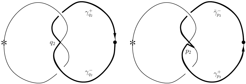
Figure 2.7. Capping paths γq2±,γp2±\gamma_{q_{2}}^{\pm},\gamma_{p_{2}}^{\pm} of q2,p2q_{2},p_{2} for the Legendrian knot from Figure 2.3.
Example.

For Λ0\Lambda_{0}, the capping paths for p2,q2p_{2},q_{2} are depicted in Figure 2.7, leading to dstr​(q2)=−q1​p1​q2+q2​p3​q3d_{\operatorname{str}}(q_{2})=-q_{1}p_{1}q_{2}+q_{2}p_{3}q_{3} and dstr​(p2)=−p3​q3​p2−p2​q2​p2−p2​q1​p1d_{\operatorname{str}}(p_{2})=-p_{3}q_{3}p_{2}-p_{2}q_{2}p_{2}-p_{2}q_{1}p_{1}. The full string differential is given below.

Theorem 2.25.

(𝒜^,d=dSFT+dstr)(\hat{\mathcal{A}},d=d_{\operatorname{SFT}}+d_{\operatorname{str}}) is an LSFT algebra.

The fact that dd preserves the filtration on 𝒜^\hat{\mathcal{A}} follows from the facts that dSFTd_{\operatorname{SFT}} and dstrd_{\operatorname{str}} also preserve the filtration; this property for dSFTd_{\operatorname{SFT}} has already been established, while for dstrd_{\operatorname{str}} this is clear by construction.

Theorem 2.25 is the LSFT analogue of the d2=0d^{2}=0 result in Legendrian contact homology, and indeed implies it. It will be proven in Section 3; see Proposition 3.15.

Example.

For Λ0\Lambda_{0}, the full derivation dd is given by

d⁡(p1)\displaystyle d(p_{1}) =−p2+(−p3​q3​p1−p2​q2​p1)\displaystyle=-p_{2}+(-p_{3}q_{3}p_{1}-p_{2}q_{2}p_{1})
d⁡(q1)\displaystyle d(q_{1}) =1+t+p3​q2+q2​p3​t+(−q1​p1​q1−q1​p2​q2−q1​p3​q3)\displaystyle=1+t+p_{3}q_{2}+q_{2}p_{3}t+(-q_{1}p_{1}q_{1}-q_{1}p_{2}q_{2}-q_{1}p_{3}q_{3})
d⁡(p2)\displaystyle d(p_{2}) =−p1​p3−p3​t​p1+(−p3​q3​p2−p2​q2​p2−p2​q1​p1)\displaystyle=-p_{1}p_{3}-p_{3}tp_{1}+(-p_{3}q_{3}p_{2}-p_{2}q_{2}p_{2}-p_{2}q_{1}p_{1})
d⁡(q2)\displaystyle d(q_{2}) =−q1+q3+(−q1​p1​q2+q2​p3​q3)\displaystyle=-q_{1}+q_{3}+(-q_{1}p_{1}q_{2}+q_{2}p_{3}q_{3})
d⁡(p3)\displaystyle d(p_{3}) =p2+(p3​q2​p2+p3​q1​p1)\displaystyle=p_{2}+(p_{3}q_{2}p_{2}+p_{3}q_{1}p_{1})
d⁡(q3)\displaystyle d(q_{3}) =1+t+q2​p1+t​p1​q2+(−q1​p1​q3−q2​p2​q3−q3​p3​q3)\displaystyle=1+t+q_{2}p_{1}+tp_{1}q_{2}+(-q_{1}p_{1}q_{3}-q_{2}p_{2}q_{3}-q_{3}p_{3}q_{3})
d⁡(t)\displaystyle d(t) =(−q1​p1​t−q2​p2​t−q3​p3​t+t​p1​q1+t​p2​q2+t​p3​q3),\displaystyle=(-q_{1}p_{1}t-q_{2}p_{2}t-q_{3}p_{3}t+tp_{1}q_{1}+tp_{2}q_{2}+tp_{3}q_{3}),

where the dstrd_{\operatorname{str}} contributions are enclosed in parentheses. The curvature for this differential is Fd=−p1−p3−p3​q2​p1F_{d}=-p_{1}-p_{3}-p_{3}q_{2}p_{1}, and indeed it is straightforward to check that d2​s=[−p1−p3−p3​q2​p1,s]d^{2}s=[-p_{1}-p_{3}-p_{3}q_{2}p_{1},s] for all generators ss of the algebra, whence d2​x=[−p1−p3−p3​q2​p1,x]d^{2}x=[-p_{1}-p_{3}-p_{3}q_{2}p_{1},x] for all x∈𝒜^x\in\hat{\mathcal{A}}.

Refer to caption

Figure 2.8. Two Legendrian unknots, the standard one with t​b=−1tb=-1 and r=0r=0 (left) and a once-stabilized one with t​b=−2tb=-2 and r=1r=1 (right).
Example.

For reference and comparison, we give here the derivations for the standard Legendrian unknot and a once-stabilized Legendrian unknot with r=1r=1, as shown in Figure 2.8. The former has

d⁡(p)\displaystyle d(p) =0\displaystyle=0
d⁡(q)\displaystyle d(q) =1+t−q​p​q\displaystyle=1+t-qpq
d⁡(t)\displaystyle d(t) =−q​p​t+t​p​q\displaystyle=-qpt+tpq

and |p|=−2|p|=-2, |q|=1|q|=1, |t|=0|t|=0, Fd=−pF_{d}=-p; the latter has

d⁡(p1)\displaystyle d(p_{1}) =q2​p2​p1−p1​p2​q2\displaystyle=q_{2}p_{2}p_{1}-p_{1}p_{2}q_{2}
d⁡(q1)\displaystyle d(q_{1}) =t−p2+p2​q2​q1−q1​p1​q1+q1​q2​p2\displaystyle=t-p_{2}+p_{2}q_{2}q_{1}-q_{1}p_{1}q_{1}+q_{1}q_{2}p_{2}
d⁡(p2)\displaystyle d(p_{2}) =0\displaystyle=0
d⁡(q2)\displaystyle d(q_{2}) =1−p1+q2​p2​q2\displaystyle=1-p_{1}+q_{2}p_{2}q_{2}
d⁡(t)\displaystyle d(t) =p2​q2​t−q1​p1​t+t​p1​q1−t​q2​p2\displaystyle=p_{2}q_{2}t-q_{1}p_{1}t+tp_{1}q_{1}-tq_{2}p_{2}

and |p1|=0|p_{1}|=0, |q1|=−1|q_{1}|=-1, |p2|=−2|p_{2}|=-2, |q2|=1|q_{2}|=1, |t|=−2|t|=-2, Fd=p2F_{d}=p_{2}.

We next state the invariance result for LSFT algebras. Our invariance proof requires us to restrict to a special class of Legendrian isotopies, though we will see that this restriction covers all Legendrian isotopies if we instead restrict to particular types of x​yxy projections.

Definition 2.26.

Two x​yxy projections Λ1,Λ2\Lambda_{1},\Lambda_{2} of Legendrian knots are related by a restricted Reidemeister II move if there is an embedded disk D⊂ℝ3D\subset\mathbb{R}^{3} such that Λ1,Λ2\Lambda_{1},\Lambda_{2} are identical outside DD, each with exactly one crossing outside DD, Λ1∩∂D=Λ2∩∂D\Lambda_{1}\cap\partial D=\Lambda_{2}\cap\partial D consists of two points, and Λ1∩D,Λ2∩D\Lambda_{1}\cap D,\Lambda_{2}\cap D are related by a Reidemeister II move inside DD. See Figure 2.9.

Two x​yxy projections are related by restricted Reidemeister moves if they are related by a sequence of Reidemeister III moves and restricted Reidemeister II moves; a restricted Legendrian isotopy is a Legendrian isotopy given in the x​yxy projection by restricted Reidemeister moves.

Refer to caption

Figure 2.9. Restricted Reidemeister II move.

Note that the Legendrian knot in Figure 2.3 is related to the standard one-crossing unknot by a Reidemeister II move eliminating crossings 22 and 33, but this move is not a restricted Reidemeister II move. It is clear that the knot from Figure 2.3 is not related to the standard unknot by restricted Reidemeister moves, though one can show that its LSFT algebra is equivalent to that of the standard unknot.

Recall that there is a standard procedure, called “morsification” [Fer02] or “resolution” [Ng03], to obtain an x​yxy projection from a front (x​zxz) projection of a Legendrian knot, by smoothing out left cusps and replacing right cusps by loops.

Proposition 2.27.

The resolutions of the fronts of two Legendrian isotopic knots can be related by restricted Reidemeister moves.

Proof.

Examine the resolutions of Legendrian Reidemeister moves for fronts: front Reidemeister III resolves to a usual Reidemeister III move; front Reidemeister I and II both resolve to Reidemeister II moves that are restricted since they do not involve the rightmost cusp of the front. ∎

The next result is the LSFT version of invariance, and again implies the analogous result in contact homology.

Theorem 2.28.

If Λ\Lambda and Λ′\Lambda^{\prime} are related by restricted Legendrian isotopy, then the LSFT algebras for Λ\Lambda and Λ′\Lambda^{\prime} are equivalent.

Theorem 2.28 will be proved in Section 4.

Corollary 2.29.

The LSFT algebra associated to the resolution of a Legendrian front is an invariant of the corresponding Legendrian knot.

As mentioned in the Introduction, it is not unreasonable to guess that one can extend Theorem 2.28 to cover all Legendrian isotopies and not just restricted ones, but one might need to broaden the notion of equivalence to allow arbitrary curved A∞A_{\infty} morphisms.

Corollary 2.30.

The stable tame isomorphism type of the contact homology DGA (ℱ0​𝒜^/ℱ1​𝒜^,d)(\mathcal{F}^{0}\!\hat{\mathcal{A}}/\mathcal{F}^{1}\!\hat{\mathcal{A}},d) is invariant under restricted Legendrian isotopy.

In fact, an examination of the proof of Theorem 2.28 shows that the contact homology DGA is invariant under all Legendrian isotopies, not just restricted ones; this recovers the original result of [Che02].

Remark 2.31 (The LSFT algebra and Legendrian contact homology).

In Remark 2.7, we identified ℱ0​𝒜^/ℱ1​𝒜^\mathcal{F}^{0}\!\hat{\mathcal{A}}/\mathcal{F}^{1}\!\hat{\mathcal{A}} with the Chekanov–Eliashberg differential graded algebra [Che02, Eli98] calculating Legendrian contact homology. This holds not only in Chekanov’s original formulation over ℤ/2\mathbb{Z}/2, but also over ℤ\mathbb{Z} in the formulation of [EES05a, EES07, ENS02]. There are, however, two caveats to this identification. First, the signs used here do not coincide precisely with the signs from [ENS02], though they do agree with another sign assignment for Legendrian contact homology given in [EES05b]. However, up to a basis change, all possible sign assignments are equivalent. The precise statement is given and proven in Appendix A.

Second, there is a base ring issue. In the standard formulation of Legendrian contact homology, the differential graded algebra is generated by Reeb chords (the qjq_{j}’s) over the group ring ℤ​[H1​(Λ)]\mathbb{Z}[H_{1}(\Lambda)], which for knots is ℤ⁡[t,t−1]\mathbb{Z}[t,t^{-1}]. In particular, t±1t^{\pm 1} commutes with all of the qjq_{j}’s. By contrast, ℱ0​𝒜^/ℱ1​𝒜^\mathcal{F}^{0}\!\hat{\mathcal{A}}/\mathcal{F}^{1}\!\hat{\mathcal{A}} is generated by the qjq_{j}’s and also t±1t^{\pm 1}, with d⁡(t±1)=0d(t^{\pm 1})=0, and t±1t^{\pm 1} does not commute with the qjq_{j}’s. We can think of the contact homology differential graded algebra as a quotient of ℱ0​𝒜^/ℱ1​𝒜^\mathcal{F}^{0}\!\hat{\mathcal{A}}/\mathcal{F}^{1}\!\hat{\mathcal{A}} by commutators involving t±1t^{\pm 1}.

On the other hand, there is no obvious reason why, in formulating Legendrian contact homology, we should impose the relation that tt commutes with the qjq_{j}’s. One could reasonably define Legendrian contact homology (even in situations more general than knots in ℝ3\mathbb{R}^{3}) without this relation. In our case, we would precisely recover ℱ0​𝒜^/ℱ1​𝒜^\mathcal{F}^{0}\!\hat{\mathcal{A}}/\mathcal{F}^{1}\!\hat{\mathcal{A}}.

2.4. The cyclic and commutative complexes

We now discuss two quotient complexes that can be derived from the LSFT algebra or any curved dg-algebra. The cyclic complex has close relations to string topology and the geometric motivation for the LSFT algebra; see Section 3.33 3 Cyclic constructions are common in Symplectic Field Theory and related topics. See for instance [BEE]. The commutative complex may be useful from a computational standpoint, especially since it has a particularly simple formulation in the case of the LSFT algebra, as we discuss at the end of this section.

Definition 2.32.

Let (𝒜^,d,F)(\hat{\mathcal{A}},d,F) be a curved dg-algebra.

  1. (1)

    Let ℐ\mathcal{I} be the submodule of 𝒜^\hat{\mathcal{A}} generated (over ℤ\mathbb{Z}, not over 𝒜^\hat{\mathcal{A}}) by commutators44 4 The restriction that one of x,y∈ℱ1​𝒜^x,y\in\mathcal{F}^{1}\!\hat{\mathcal{A}} is unnecessary for most purposes, but is needed for the theory to include full Legendrian contact homology, rather than a cyclic version, as a quotient.

    {[x,y]|x,y∈𝒜^ and at least one of x,y∈ℱ1​𝒜^}.\{[x,y]\,|\,x,y\in\hat{\mathcal{A}}\text{ and at least one of $x,y\in\mathcal{F}^{1}\!\hat{\mathcal{A}}$}\}.

    The cyclic complex associated to (𝒜^,d,F)(\hat{\mathcal{A}},d,F) is (𝒜^cyc=𝒜^/ℐ,d)(\hat{\mathcal{A}}^{\operatorname{cyc}}=\hat{\mathcal{A}}/\mathcal{I},d), where dd is the induced differential on 𝒜^cyc\hat{\mathcal{A}}^{\operatorname{cyc}}.

  2. (2)

    Let 𝒥\mathcal{J} be the subalgebra of 𝒜^\hat{\mathcal{A}} generated (over 𝒜^\hat{\mathcal{A}}) by commutators [x,y][x,y] for all x,y∈𝒜^x,y\in\hat{\mathcal{A}}. The commutative complex associated to (𝒜^,d,F)(\hat{\mathcal{A}},d,F) is (𝒜^comm=𝒜^/𝒥,d)(\hat{\mathcal{A}}^{\operatorname{comm}}=\hat{\mathcal{A}}/\mathcal{J},d), where dd is the induced differential on 𝒜^comm\hat{\mathcal{A}}^{\operatorname{comm}}.

The key point here is that d2=0d^{2}=0 on 𝒜^cyc\hat{\mathcal{A}}^{\operatorname{cyc}} and 𝒜^comm\hat{\mathcal{A}}^{\operatorname{comm}}, by the definition of curved dg-algebra.

When 𝒜^\hat{\mathcal{A}} is a tensor algebra (as for the LSFT algebra), 𝒜^cyc\hat{\mathcal{A}}^{\operatorname{cyc}} is generated by “cyclic words”, or words modulo cyclic permutations of the letters (for words in ℱ1​𝒜^\mathcal{F}^{1}\!\hat{\mathcal{A}}). Note that 𝒜^cyc\hat{\mathcal{A}}^{\operatorname{cyc}} is a ℤ\mathbb{Z}-module and not an algebra; it however still inherits the grading and filtration from 𝒜^\hat{\mathcal{A}}. By contrast, 𝒜^comm\hat{\mathcal{A}}^{\operatorname{comm}} is a (sign-)commutative algebra over ℤ\mathbb{Z}, the polynomial algebra generated by the generators of 𝒜^\hat{\mathcal{A}}. There are obvious quotient maps

(𝒜^,d,F)\textstyle{(\hat{\mathcal{A}},d,F)\ignorespaces\ignorespaces\ignorespaces\ignorespaces}(𝒜^cyc,d)\textstyle{(\hat{\mathcal{A}}^{\operatorname{cyc}},d)\ignorespaces\ignorespaces\ignorespaces\ignorespaces}(𝒜^comm,d),\textstyle{(\hat{\mathcal{A}}^{\operatorname{comm}},d),}

and the latter induces a map on homology.

We next show that the cyclic and commutative complexes associated to the LSFT algebra of a Legendrian knot are invariant. This is a direct consequence of the following result.

Proposition 2.33.

If (𝒜^,d)(\hat{\mathcal{A}},d) and (𝒜^′,d′)(\hat{\mathcal{A}}^{\prime},d^{\prime}) are equivalent LSFT algebras, then their rational cyclic and commutative quotient complexes are filtered chain homotopy equivalent. In particular, they are quasi-isomorphic:

H∗​(𝒜^cyc⊗ℚ,d)≅H∗​((𝒜^′)cyc⊗ℚ,d′)H_{*}(\hat{\mathcal{A}}^{\operatorname{cyc}}\otimes\mathbb{Q},d)\cong H_{*}((\hat{\mathcal{A}}^{\prime})^{\operatorname{cyc}}\otimes\mathbb{Q},d^{\prime})

as filtered graded ℚ\mathbb{Q}-modules, and

H∗​(𝒜^comm⊗ℚ,d)≅H∗​((𝒜^′)comm⊗ℚ,d′)H_{*}(\hat{\mathcal{A}}^{\operatorname{comm}}\otimes\mathbb{Q},d)\cong H_{*}((\hat{\mathcal{A}}^{\prime})^{\operatorname{comm}}\otimes\mathbb{Q},d^{\prime})

as filtered graded ℚ\mathbb{Q}-algebras.

The substance of the proof of Proposition 2.33, which we give below, is invariance under stabilization. Recall from the proof of Proposition 2.15 the maps ι,π\iota,\pi between an LSFT algebra (𝒜^,d)(\hat{\mathcal{A}},d) and its stabilization (Si​𝒜^,d)(S_{i}\hat{\mathcal{A}},d). Though the homotopy operator HH from that proof does not descend from Si​𝒜^S_{i}\hat{\mathcal{A}} to (Si​𝒜^)cyc(S_{i}\hat{\mathcal{A}})^{\text{cyc}}, we can define a slight variant that serves as the corresponding homotopy operator for (Si​𝒜^)cyc(S_{i}\hat{\mathcal{A}})^{\operatorname{cyc}}. Let h:Si​𝒜^→Si​𝒜^h\colon\thinspace S_{i}\hat{\mathcal{A}}\to S_{i}\hat{\mathcal{A}} be the derivation defined by h⁡(qb)=qah(q_{b})=q_{a}, h⁡(pa)=pbh(p_{a})=p_{b}, h⁡(qa)=h⁡(pb)=0h(q_{a})=h(p_{b})=0, h⁡(qj)=h⁡(pj)=h⁡(t±1)=0h(q_{j})=h(p_{j})=h(t^{\pm 1})=0 for all jj (besides a,ba,b). For a word w∈𝒜^w\in\hat{\mathcal{A}}, let σ⁡(w)\sigma(w) be the total number of occurrences of qa,qb,pa,pbq_{a},q_{b},p_{a},p_{b} in xx. Now define Hcyc:(Si​𝒜^)⊗ℚ→(Si​𝒜^)⊗ℚH^{\operatorname{cyc}}\colon\thinspace(S_{i}\hat{\mathcal{A}})\otimes\mathbb{Q}\to(S_{i}\hat{\mathcal{A}})\otimes\mathbb{Q} by

Hcyc​(w)={0if σ⁡(w)=01σ⁡(w)​h​(w)if σ⁡(w)>0.H^{\operatorname{cyc}}(w)=\begin{cases}0&\text{if $\sigma(w)=0$}\\ \frac{1}{\sigma(w)}h(w)&\text{if $\sigma(w)>0$}.\end{cases}
Lemma 2.34.

On (Si​𝒜^)⊗ℚ(S_{i}\hat{\mathcal{A}})\otimes\mathbb{Q}, we have IdSi​𝒜^−ι∘π=Hcyc∘d+d∘Hcyc\operatorname{Id}_{S_{i}\hat{\mathcal{A}}}-\iota\circ\pi=H^{\operatorname{cyc}}\circ d+d\circ H^{\operatorname{cyc}}.

Proof.

It suffices to show that (h∘d+d∘h)​(w)=σ⁡(w)​w(h\circ d+d\circ h)(w)=\sigma(w)w for all words ww, since dd preserves the number of occurrences of qa,qb,pa,pbq_{a},q_{b},p_{a},p_{b}. But both h∘d+d∘hh\circ d+d\circ h and the map (generated on words by) w↦σ⁡(w)​ww\mapsto\sigma(w)w are derivations, and they agree on the generators qa,qb,pa,pb,qj,pj,tq_{a},q_{b},p_{a},p_{b},q_{j},p_{j},t. ∎

Proof of Proposition 2.33.

Let (𝒜^,d)(\hat{\mathcal{A}},d) and (𝒜^′,d′)(\hat{\mathcal{A}}^{\prime},d^{\prime}) be equivalent LSFT algebras. We show that (𝒜^cyc⊗ℚ,d)(\hat{\mathcal{A}}^{\operatorname{cyc}}\otimes\mathbb{Q},d) and ((𝒜^′)cyc⊗ℚ,d′)((\hat{\mathcal{A}}^{\prime})^{\operatorname{cyc}}\otimes\mathbb{Q},d^{\prime}) are filtered chain homotopy equivalent; the proof of the corresponding result for the commutative complexes is nearly identical. The result clearly holds if (𝒜^,d)(\hat{\mathcal{A}},d) and (𝒜^′,d′)(\hat{\mathcal{A}}^{\prime},d^{\prime}) are related by a basis change or gauge change. Thus we may assume that (𝒜^′,d′)=(Si​𝒜^,d)(\hat{\mathcal{A}}^{\prime},d^{\prime})=(S_{i}\hat{\mathcal{A}},d) is a stabilization of (𝒜^,d)(\hat{\mathcal{A}},d). In this case, the inclusion and projection maps ι,π\iota,\pi between 𝒜^\hat{\mathcal{A}} and Si​𝒜^S_{i}\hat{\mathcal{A}} induce chain maps ι:𝒜^cyc→(Si​𝒜^)cyc\iota\colon\thinspace\hat{\mathcal{A}}^{\operatorname{cyc}}\to(S_{i}\hat{\mathcal{A}})^{\operatorname{cyc}} and π:(Si​𝒜^)cyc→𝒜^cyc\pi\colon\thinspace(S_{i}\hat{\mathcal{A}})^{\operatorname{cyc}}\to\hat{\mathcal{A}}^{\operatorname{cyc}}. Furthermore, π∘ι=Id𝒜^cyc\pi\circ\iota=\operatorname{Id}_{\hat{\mathcal{A}}^{\operatorname{cyc}}}, while ι∘π\iota\circ\pi is chain homotopic over ℚ\mathbb{Q} to Id(Si​𝒜^)cyc\operatorname{Id}_{(S_{i}\hat{\mathcal{A}})^{\operatorname{cyc}}} by Lemma 2.34. ∎

Corollary 2.35.

The cyclic and commutative complexes associated to the LSFT algebra of a Legendrian knot are invariant, up to filtered chain homotopy equivalence, under restricted Legendrian isotopy.

We remark that it can be checked that the powers of FF, Fn∈𝒜^F^{n}\in\hat{\mathcal{A}} for n≥0n\geq 0, descend to invariant classes in H⁡(𝒜^cyc⊗ℚ,d)H(\hat{\mathcal{A}}^{\operatorname{cyc}}\otimes\mathbb{Q},d). See [Pos93] for a fuller discussion, where these invariant classes are called “Chern classes”.

To end this section, we observe that the commutative complex for an LSFT algebra has a rather simpler formulation than the full LSFT algebra. More precisely, on 𝒜^comm\hat{\mathcal{A}}^{\operatorname{comm}} we can still define d=dSFT+dstrd=d_{\operatorname{SFT}}+d_{\operatorname{str}}, with dSFTd_{\operatorname{SFT}} defined as for 𝒜^\hat{\mathcal{A}}, but now dstrd_{\operatorname{str}} can be given as follows.

Refer to caption

Figure 2.10. A schematic diagram traversing πx​y​(Λ)\pi_{xy}(\Lambda) along its orientation. In this picture, the crossings corresponding to ss and s′s^{\prime} are interlaced, and we have s⇢s′⇢s∗⇢s′⁣∗⇢ss\dasharrow s^{\prime}\dasharrow s^{*}\dasharrow s^{\prime*}\dasharrow s.
Definition 2.36.

Two crossings in πx​y​(Λ)\pi_{xy}(\Lambda) are interlaced if, in traversing the knot one full time, we encounter one crossing, then the other, then the first again, then the second again. If crossings corresponding to ss and s′s^{\prime} are interlaced, we say that ss is interlaced toward s′s^{\prime} and write s⇢s′s\dasharrow s^{\prime} if, when we traverse Λ\Lambda along its orientation starting from s−s^{-}, we encounter (s′)−(s^{\prime})^{-} before (s′)+(s^{\prime})^{+}.

See Figure 2.10 for an illustration. If the crossings corresponding to ss and s′s^{\prime} are interlaced, then there are two possibilities, s⇢s′⇢s∗⇢s′⁣∗⇢ss\dasharrow s^{\prime}\dasharrow s^{*}\dasharrow s^{\prime*}\dasharrow s or s⇢s′⁣∗⇢s∗⇢s′⇢ss\dasharrow s^{\prime*}\dasharrow s^{*}\dasharrow s^{\prime}\dasharrow s, depending on the orientation of Λ\Lambda.

Proposition 2.37.

In 𝒜^comm\hat{\mathcal{A}}^{\operatorname{comm}}, we have dstr​(t±1)=0d_{\operatorname{str}}(t^{\pm 1})=0, while if ss is a pp or qq, then

dstr​(s)=∑s⇢s′{s′⁣∗,s′}​s′⁣∗​s′​sd_{\operatorname{str}}(s)=\sum_{s\dasharrow s^{\prime}}\{s^{\prime*},s^{\prime}\}\,s^{\prime*}s^{\prime}s

where the sum is over all s′s^{\prime} such that ss is interlaced toward s′s^{\prime}, and {s′⁣∗,s′}\{s^{\prime*},s^{\prime}\} is 11 if s′s^{\prime} is a qq, −1-1 if s′s^{\prime} is a pp.

The proof of Proposition 2.37 is an exercise in chasing signs, and we leave it to the interested reader. Note that dstrd_{\operatorname{str}} does not depend on the choice of base points ∙,∗\bullet,\ast on Λ\Lambda. Thus the differential dd on 𝒜^comm\hat{\mathcal{A}}^{\operatorname{comm}} is independent of ∙\bullet, and only depends on ∗\ast insofar as ∗\ast keeps track of powers of tt in the SFT differential, cf. group-ring coefficients in Legendrian contact homology [ENS02].

3. String Interpretation of the LSFT Algebra

It will be useful to have another description of the LSFT algebra, closer to the standard SFT formalism and string topology. This allows us to prove the “d2=0d^{2}=0 result”, Theorem 2.25.

3.1. Broken closed strings and the SFT bracket

Generators of the LSFT algebra of a Legendrian knot Λ\Lambda are more conveniently seen as strings on Λ\Lambda. From the holomorphic perspective, these are the boundaries of holomorphic disks with boundary on Λ×ℝ\Lambda\times\mathbb{R}. It will be fruitful, however, to consider all possible strings, not just those that arise as the boundary of a disk.

Definition 3.1.

Let Λ∈ℝ3\Lambda\in\mathbb{R}^{3} be a Legendrian knot with Reeb chords R1,…,RnR_{1},\dots,R_{n}, and let Ri±∈ΛR_{i}^{\pm}\in\Lambda denote the endpoints of Reeb chord RiR_{i}. For fixed k≥0k\geq 0, choose kk distinct points τ1,…,τk\tau_{1},\dots,\tau_{k} on an oriented circle S1S^{1} so that they appear sequentially in order; we refer to these points as punctures of S1S^{1}, and the punctures divide S1S^{1} into kk intervals, which we denote [τ1,τ2],[τ2,τ3],…,[τk,τ1][\tau_{1},\tau_{2}],[\tau_{2},\tau_{3}],\dots,[\tau_{k},\tau_{1}]. A broken closed string of length kk is a piecewise continuous map γ:S1→Λ\gamma\colon\thinspace S^{1}\to\Lambda such that:

  1. (1)

    γ|[τj,τj+1]\gamma|_{[\tau_{j},\tau_{j+1}]} is continuous for each jj;

  2. (2)

    for each j=1,…,kj=1,\dots,k, either limτ→τj±γ⁡(τ)=Rij±\lim_{\tau\to\tau_{j}^{\pm}}\gamma(\tau)=R_{i_{j}}^{\pm} or limτ→τj±γ⁡(τ)=Rij∓\lim_{\tau\to\tau_{j}^{\pm}}\gamma(\tau)=R_{i_{j}}^{\mp} for some iji_{j}.

We consider broken closed strings up to orientation-preserving reparametrization of the domain S1S^{1}.

If we are given a point ∙∈Λ\bullet\in\Lambda distinct from any of the Ri±R_{i}^{\pm}, then choose a point τ0∈(τk,τ1)⊂S1\tau_{0}\in(\tau_{k},\tau_{1})\subset S^{1}; a based broken closed string of length kk is a broken closed string γ\gamma of length kk such that γ(τ0)=∙\gamma(\tau_{0})=\bullet.

Given distinct points ∗,∙∈Λ\ast,\bullet\in\Lambda, we obtain a map ww between based broken closed strings and words in 𝒜^\hat{\mathcal{A}}. If γ\gamma is a based broken closed string of length kk, then define the word associated to γ\gamma to be

w(γ)=ta0s1ta1s2⋯sktakw(\gamma)=t^{a_{0}}s_{1}t^{a_{1}}s_{2}\cdots s_{k}t^{a_{k}}

where tajt^{a_{j}} is the number of times γ|[τj,τj+1]\gamma|_{[\tau_{j},\tau_{j+1}]} passes through ∗\ast, counted with sign according to the orientation of Λ\Lambda, and

sj={pijif limτ→τj±γ⁡(τ)=Rij±qijif limτ→τj±γ⁡(τ)=Rij∓.s_{j}=\begin{cases}p_{i_{j}}&\text{if $\lim_{\tau\to\tau_{j}^{\pm}}\gamma(\tau)=R_{i_{j}}^{\pm}$}\\ q_{i_{j}}&\text{if $\lim_{\tau\to\tau_{j}^{\pm}}\gamma(\tau)=R_{i_{j}}^{\mp}$}.\end{cases}

Note that the correspondence between based broken closed strings and words in 𝒜^\hat{\mathcal{A}} is bijective if we mod out the strings by homotopy.

Similarly, we can define a map, which we also denote by ww, between broken closed strings and words in 𝒜^cyc\hat{\mathcal{A}}^{\operatorname{cyc}}. Note that this map does not depend on the choice of ∙\bullet, as changing ∙\bullet corresponds to conjugation by some power of tt.

If γ,γ′\gamma,\gamma^{\prime} are broken closed strings of length k,k′k,k^{\prime} respectively, and a puncture from each is mapped to (the endpoints of) the same Reeb chord but in opposite directions, then we can glue γ,γ′\gamma,\gamma^{\prime} at this puncture to obtain another broken closed string of length k+k′−2k+k^{\prime}-2. More precisely, suppose that the S1S^{1} domain of γ\gamma has punctures τ1,…,τk\tau_{1},\dots,\tau_{k}, the S1S^{1} domain of γ′\gamma^{\prime} has punctures τ1′,…,τk′′\tau_{1}^{\prime},\dots,\tau_{k^{\prime}}^{\prime}, and there are jj and j′j^{\prime} such that

limτ→τj±γ⁡(τ)=limτ→τj′∓γ′​(τ);\lim_{\tau\to\tau_{j}^{\pm}}\gamma(\tau)=\lim_{\tau\to\tau_{j^{\prime}}^{\mp}}\gamma^{\prime}(\tau);

then we can define a broken closed string γ∗γ′\gamma*\gamma^{\prime} on S1S^{1} with sequential punctures τj+1,…,τk,τ1,…,τj−1,τj′+1′,…,τk′′,τ1′,…,τj′−1′\tau_{j+1},\dots,\tau_{k},\tau_{1},\dots,\tau_{j-1},\tau_{j^{\prime}+1}^{\prime},\dots,\tau_{k^{\prime}}^{\prime},\tau_{1}^{\prime},\dots,\tau_{j^{\prime}-1}^{\prime} by

(γ∗γ′)|[τi,τi+1]\displaystyle(\gamma*\gamma^{\prime})|_{[\tau_{i},\tau_{i+1}]} =γ|[τi,τi+1]\displaystyle=\gamma|_{[\tau_{i},\tau_{i+1}]}
for all i=1,…,ki=1,\dots,k with i≠ji\neq j,
(γ∗γ′)|[τi′,τi+1′]\displaystyle(\gamma*\gamma^{\prime})|_{[\tau_{i}^{\prime},\tau_{i+1}^{\prime}]} =γ′|[τi′,τi+1′]\displaystyle=\gamma^{\prime}|_{[\tau_{i}^{\prime},\tau_{i+1}^{\prime}]}
for all i=1,…,k′i=1,\dots,k^{\prime} with i≠j′i\neq j^{\prime},
(γ∗γ′)|[τj−1,τj′+1′]\displaystyle(\gamma*\gamma^{\prime})|_{[\tau_{j-1},\tau_{j^{\prime}+1}^{\prime}]} =γ|[τj−1,τj]∪γ′|[τj′′,τj′+1′],\displaystyle=\gamma|_{[\tau_{j-1},\tau_{j}]}\cup\gamma^{\prime}|_{[\tau_{j^{\prime}}^{\prime},\tau_{j^{\prime}+1}^{\prime}]},
(γ∗γ′)|[τj′−1′,τj+1]\displaystyle(\gamma*\gamma^{\prime})|_{[\tau_{j^{\prime}-1}^{\prime},\tau_{j+1}]} =γ′|[τj′−1′,τj′′]∪γ|[τj,τj+1].\displaystyle=\gamma^{\prime}|_{[\tau_{j^{\prime}-1}^{\prime},\tau_{j^{\prime}}^{\prime}]}\cup\gamma|_{[\tau_{j},\tau_{j+1}]}.

See Figure 3.1 for an illustration.

Refer to caption

Figure 3.1. Gluing broken closed strings γ,γ′\gamma,\gamma^{\prime} at punctures τ3,τ2′\tau_{3},\tau_{2}^{\prime} to produce a new broken closed string γ∗γ′\gamma*\gamma^{\prime}. The top illustrates the picture in the domain; the bottom illustrates the image of γ,γ′,γ∗γ′\gamma,\gamma^{\prime},\gamma*\gamma^{\prime} in the x​yxy projection πx​y​(Λ)\pi_{xy}(\Lambda). The heavy bar indicates the glued corners.

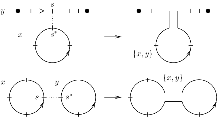
Using the gluing operation, we can define the SFT bracket of two broken closed strings to be the sum of all possible gluings of the broken closed strings. This gives an operation {⋅,⋅}:𝒜^cyc⊗𝒜^cyc→𝒜^cyc\{\cdot,\cdot\}\colon\thinspace\hat{\mathcal{A}}^{\operatorname{cyc}}\otimes\hat{\mathcal{A}}^{\operatorname{cyc}}\to\hat{\mathcal{A}}^{\operatorname{cyc}} (at least mod 22). In the same way, we can define the SFT bracket of a broken closed string and a based broken closed string to be the sum of all based broken closed strings obtained by gluing; this gives a mod 22 map {⋅,⋅}:𝒜^cyc⊗𝒜^→𝒜^\{\cdot,\cdot\}\colon\thinspace\hat{\mathcal{A}}^{\operatorname{cyc}}\otimes\hat{\mathcal{A}}\to\hat{\mathcal{A}}. We refer to either operation as the SFT bracket. See Figure 3.2.
Refer to caption

Figure 3.2. Gluing x∈𝒜^cycx\in\hat{\mathcal{A}}^{\operatorname{cyc}} to y∈𝒜^y\in\hat{\mathcal{A}} to get {x,y}∈𝒜^\{x,y\}\in\hat{\mathcal{A}} (top); gluing x∈𝒜^cycx\in\hat{\mathcal{A}}^{\operatorname{cyc}} to y∈𝒜^cycy\in\hat{\mathcal{A}}^{\operatorname{cyc}} to get {x,y}∈𝒜^cyc\{x,y\}\in\hat{\mathcal{A}}^{\operatorname{cyc}} (bottom). The notches represent corners (punctures), and the dots represent the base point ∙\bullet.

We can define the SFT bracket in a more precise algebraic manner, with the added benefit of lifting to ℤ\mathbb{Z}, as follows. First, given a word w∈𝒜w\in\mathcal{A} ending in a pp or qq, define a contraction map ιw:𝒜→𝒜\iota_{w}\colon\thinspace\mathcal{A}\to\mathcal{A} as follows. Write w=w′​piw=w^{\prime}p_{i} or w=w′​qiw=w^{\prime}q_{i} for some word w′w^{\prime}, and set

ιw′​pi​(s)={δi​j​w′if x=qj0if x=pj or x=t±1\iota_{w^{\prime}p_{i}}(s)=\begin{cases}\delta_{ij}w^{\prime}&\text{if $x=q_{j}$}\\ 0&\text{if $x=p_{j}$ or $x=t^{\pm 1}$}\end{cases}

and

ιw′​qi​(x)={−δi​j​w′if x=pj0if x=qj or x=t±1,\iota_{w^{\prime}q_{i}}(x)=\begin{cases}-\delta_{ij}w^{\prime}&\text{if $x=p_{j}$}\\ 0&\text{if $x=q_{j}$ or $x=t^{\pm 1}$},\end{cases}

where δi​j\delta_{ij} is the Kronecker delta function; extend ιw\iota_{w} to a map 𝒜→𝒜\mathcal{A}\to\mathcal{A} by linearity and the following modified Leibniz rule:

ιw​(x​y)=(ιw​x)​y+(−1)(|w|+1)​|x|​x​(ιw​y).\iota_{w}(xy)=(\iota_{w}x)y+(-1)^{(|w|+1)|x|}x(\iota_{w}y).

The unusual sign ensures that ιw\iota_{w} descends to a map 𝒜cyc→𝒜cyc\mathcal{A}^{\operatorname{cyc}}\to\mathcal{A}^{\operatorname{cyc}}.

Before extending contraction to cyclic words and defining the SFT bracket, we introduce notation for the set of all words that project to a particular cyclic word.

Definition 3.2.

Let ww be a word in 𝒜\mathcal{A}. The length l⁡(w)l(w) of ww is the number of qq’s and pp’s in ww. The cyclic word set 𝒞⁡(w)\mathcal{C}(w) of ww is the l⁡(w)l(w)-element multiset in 𝒜^\hat{\mathcal{A}} of words equal to ww in 𝒜^cyc\hat{\mathcal{A}}^{\operatorname{cyc}}. More precisely, if w=ta0s1ta1s2⋯sl⁡(w)tal⁡(w)w=t^{a_{0}}s_{1}t^{a_{1}}s_{2}\cdots s_{l(w)}t^{a_{l(w)}}, where each sis_{i} is a qq or pp, then

𝒞⁡(w)\displaystyle\mathcal{C}(w) ={ta0+al⁡(w)s1ta1s2⋯sl⁡(w),\displaystyle=\left\{t^{a_{0}+a_{l(w)}}s_{1}t^{a_{1}}s_{2}\cdots s_{l(w)},\right.
(−1)|s1|​(|w|−|s1|)ta1s2⋯sl⁡(w)ta0+al⁡(w)s1,…,\displaystyle(-1)^{|s_{1}|(|w|-|s_{1}|)}t^{a_{1}}s_{2}\cdots s_{l(w)}t^{a_{0}+a_{l(w)}}s_{1},\dots,
(−1)|sl⁡(w)|​(|w|−|sl⁡(w)|)tal⁡(w)−1sl⁡(w)ta0+al⁡(w)s1⋯sl⁡(w)−1}.\displaystyle\left.(-1)^{|s_{l(w)}|(|w|-|s_{l(w)}|)}t^{a_{l(w)-1}}s_{l(w)}t^{a_{0}+a_{l(w)}}s_{1}\cdots s_{l(w)-1}\right\}.

Note that if w,w′w,w^{\prime} represent the same element in 𝒜^cyc\hat{\mathcal{A}}^{\operatorname{cyc}}, then 𝒞⁡(w)=𝒞⁡(w′)\mathcal{C}(w)=\mathcal{C}(w^{\prime}).

Now if ww is a word in 𝒜\mathcal{A} and [w][w] is the image of ww in 𝒜cyc\mathcal{A}^{\operatorname{cyc}}, then we define a contraction map ι[w]:𝒜^→𝒜^\iota_{[w]}\colon\thinspace\hat{\mathcal{A}}\to\hat{\mathcal{A}} by

ι[w]​(x)=∑y∈𝒞⁡(w)ιy​(x).\iota_{[w]}(x)=\sum_{y\in\mathcal{C}(w)}\iota_{y}(x).

Here we use the convention that ι−w​(x)=−ιw​(x)\iota_{-w}(x)=-\iota_{w}(x) if ww is a word in 𝒜\mathcal{A}. The contraction map extends by linearity to a map ι⋅​(⋅):𝒜^cyc⊗𝒜^→𝒜^\iota_{\cdot}(\cdot)\colon\thinspace\hat{\mathcal{A}}^{\operatorname{cyc}}\otimes\hat{\mathcal{A}}\to\hat{\mathcal{A}}.

Definition 3.3.

The SFT bracket {⋅,⋅}:𝒜^cyc⊗𝒜^→𝒜^\{\cdot,\cdot\}\colon\thinspace\hat{\mathcal{A}}^{\operatorname{cyc}}\otimes\hat{\mathcal{A}}\to\hat{\mathcal{A}} is defined by {x,y}=ιx​(y)\{x,y\}=\iota_{x}(y). This descends to a map 𝒜^cyc⊗𝒜^cyc→𝒜^cyc\hat{\mathcal{A}}^{\operatorname{cyc}}\otimes\hat{\mathcal{A}}^{\operatorname{cyc}}\to\hat{\mathcal{A}}^{\operatorname{cyc}}, which we also denote by {⋅,⋅}\{\cdot,\cdot\}.

For reference, the full sign rule, which can be deduced from the definition of ι\iota, is as follows: the ss and s∗s^{*} entries in two words w1​s​w2w_{1}sw_{2}, w3​s∗​w4w_{3}s^{*}w_{4} pair together to give

(3) {w1​s​w2,w3​s∗​w4}=(−1)|w2|​|w1​s|+(|w1​s​w2|+1)​|w3|​{s,s∗}​w3​w2​w1​w4+⋯.\{w_{1}sw_{2},w_{3}s^{*}w_{4}\}=(-1)^{|w_{2}||w_{1}s|+(|w_{1}sw_{2}|+1)|w_{3}|}\{s,s^{*}\}w_{3}w_{2}w_{1}w_{4}+\cdots.
Proposition 3.4 (Properties of the SFT bracket).
  1. (1)

    Let x,y∈𝒜^cycx,y\in\hat{\mathcal{A}}^{\operatorname{cyc}}. Then

    {y,x}=(−1)|x|​|y|+|x|+|y|​{x,y}.\{y,x\}=(-1)^{|x||y|+|x|+|y|}\{x,y\}.
  2. (2)

    Let x∈𝒜^cycx\in\hat{\mathcal{A}}^{\operatorname{cyc}} and y,z∈𝒜^y,z\in\hat{\mathcal{A}}. Then

    {x,y​z}={x,y}​z+(−1)(|x|+1)​|y|​y​{x,z}.\{x,yz\}=\{x,y\}z+(-1)^{(|x|+1)|y|}y\{x,z\}.
  3. (3)

    Let x,y∈𝒜^cycx,y\in\hat{\mathcal{A}}^{\operatorname{cyc}} and z∈𝒜^z\in\hat{\mathcal{A}}. Then we have the following version of the Jacobi identity:

    {x,{y,z}}+(−1)|x|​|y|+|x|+|y|​{y,{x,z}}={{x,y},z}.\{x,\{y,z\}\}+(-1)^{|x||y|+|x|+|y|}\{y,\{x,z\}\}=\{\{x,y\},z\}.
Proof.

We first establish the proposition mod 22. Note that (1) is clear, while (2) can be pictorially represented:

{x,y​z}=[Uncaptioned image]=[Uncaptioned image]+[Uncaptioned image]={x,y}​z+y⁡{x,z}.\{x,yz\}=\raisebox{-11.0pt}{\includegraphics[height=33.0pt]{figures/sftb1.eps}}=\raisebox{-11.0pt}{\includegraphics[height=33.0pt]{figures/sftb2.eps}}+\raisebox{-11.0pt}{\includegraphics[height=33.0pt]{figures/sftb3.eps}}=\{x,y\}z+y\{x,z\}.

For (3), we have

{x,{y,z}}\displaystyle\{x,\{y,z\}\} =[Uncaptioned image]+[Uncaptioned image]+[Uncaptioned image]\displaystyle=\raisebox{-11.0pt}{\includegraphics[height=33.0pt]{figures/sftb4.eps}}+\raisebox{-11.0pt}{\includegraphics[height=33.0pt]{figures/sftb5.eps}}+\raisebox{-11.0pt}{\includegraphics[height=33.0pt]{figures/sftb6.eps}}
{y,{x,z}}\displaystyle\{y,\{x,z\}\} =[Uncaptioned image]+[Uncaptioned image]+[Uncaptioned image]\displaystyle=\raisebox{-11.0pt}{\includegraphics[height=33.0pt]{figures/sftb4.eps}}+\raisebox{-11.0pt}{\includegraphics[height=33.0pt]{figures/sftb5.eps}}+\raisebox{-11.0pt}{\includegraphics[height=33.0pt]{figures/sftb7.eps}}
{{x,y},z}\displaystyle\{\{x,y\},z\} =[Uncaptioned image]+[Uncaptioned image].\displaystyle=\raisebox{-11.0pt}{\includegraphics[height=33.0pt]{figures/sftb7.eps}}+\raisebox{-11.0pt}{\includegraphics[height=33.0pt]{figures/sftb6.eps}}.

Checking the signs is now a routine exercise using equation (3). ∎

3.2. The δ\delta map

Having defined the SFT bracket, we now define another operation on strings, the δ\delta map. This is essentially a string cobracket operation in the language of string topology. First we need to take a slightly closer look at broken closed strings.

Definition 3.5.

A generic broken closed string is a broken closed string γ:(S1,τ1,…,τk)→Λ\gamma\colon\thinspace(S^{1};\tau_{1},\dots,\tau_{k})\to\Lambda such that whenever γ′​(τ)=0\gamma^{\prime}(\tau)=0, γ⁡(τ)∉ℛ\gamma(\tau)\not\in\mathcal{R}, where we recall that ℛ\mathcal{R} is the set of Reeb chord endpoints; in particular, γ′​(τi±)≠0\gamma^{\prime}({\tau_{i}}^{\pm})\neq 0, where γ′​(τi±)=limτ→τi±γ′​(τ)\gamma^{\prime}(\tau_{i}^{\pm})=\lim_{\tau\to\tau_{i}^{\pm}}\gamma^{\prime}(\tau).

A generic broken closed string has holomorphic corners if for each ii, (γ′​(τi−),γ⁡(τi+)−γ⁡(τi−),γ′​(τi+))(\gamma^{\prime}(\tau_{i}^{-}),\gamma(\tau_{i}^{+})-\gamma(\tau_{i}^{-}),\gamma^{\prime}(\tau_{i}^{+})) is a positively oriented frame in ℝ3\mathbb{R}^{3}. This condition is most easily interpreted in the x​yxy projection: the image of γ\gamma in πx​y​(Λ)\pi_{xy}(\Lambda) near each τi\tau_{i} makes a left turn at the corner.

Refer to caption

Figure 3.3. From left to right: a holomorphic corner of a broken closed string; a non-holomorphic corner; and two broken closed strings with holomorphic corners homotopic to the one with the non-holomorphic corner.

Refer to caption

Figure 3.4. A generic broken closed string γ\gamma with holomorphic corners. The word associated to γ\gamma is p2​t​p1p_{2}tp_{1}.

See Figure 3.3 for an illustration of holomorphic corners and Figure 3.4 for an example of a generic broken closed string with holomorphic corners. It is easy to see that any broken closed string is homotopic to a generic broken closed string with holomorphic corners.

Now suppose that γ:(S1,τ1,…,τk)→Λ\gamma\colon\thinspace(S^{1};\tau_{1},\dots,\tau_{k})\to\Lambda is a generic broken closed string of length kk, and suppose τ∈(τi,τi+1)\tau\in(\tau_{i},\tau_{i+1}) satisfies γ⁡(τ)=Rj±\gamma(\tau)=R_{j}^{\pm} for some jj and some choice of ±\pm; in this case, we say that τ\tau is interior Reeb for γ\gamma. We can then define a broken closed string δ⁡(γ,τ)\delta(\gamma;\tau) of length k+2k+2 to have sequential punctures τ1,…,τi,τ(1),τ(2),τi+1,…,τk\tau_{1},\dots,\tau_{i},\tau^{(1)},\tau^{(2)},\tau_{i+1},\dots,\tau_{k}, and

δ⁡(γ,τ)|[τi,τ(1)]\displaystyle\delta(\gamma;\tau)|_{[\tau_{i},\tau^{(1)}]} =γ|[τi,t]\displaystyle=\gamma|_{[\tau_{i},t]}
δ⁡(γ,τ)|[τ(1),τ(2)]\displaystyle\delta(\gamma;\tau)|_{[\tau^{(1)},\tau^{(2)}]} =constant path at Rj∓\displaystyle=\text{constant path at $R_{j}^{\mp}$}
δ⁡(γ,τ)|[τ(2),τi+1]\displaystyle\delta(\gamma;\tau)|_{[\tau^{(2)},\tau_{i+1}]} =γ|[τ,τi+1]\displaystyle=\gamma|_{[\tau,\tau_{i+1}]}
δ⁡(γ,τ)|[τj,τj+1]\displaystyle\delta(\gamma;\tau)|_{[\tau_{j},\tau_{j+1}]} =γ|[τj,τj+1]for j≠i.\displaystyle=\gamma|_{[\tau_{j},\tau_{j+1}]}\quad\text{for $j\neq i$.}

Note that δ⁡(γ,τ)\delta(\gamma;\tau) is not generic, but it can be perturbed to become generic; furthermore, if we stipulate that the perturbed broken closed string has holomorphic corners on the domain interval (τi,τi+1)(\tau_{i},\tau_{i+1}), then the perturbation is unique up to homotopy through generic broken closed strings with holomorphic corners.

If γ\gamma is a generic based broken closed curve and τ\tau is interior Reeb for γ\gamma, we can similarly define a based broken closed curve δ⁡(γ,τ)\delta(\gamma;\tau).

Refer to caption

Figure 3.5. The three terms in δ⁡(p2​t​p1)\delta(p_{2}tp_{1}) for the broken closed string γ=γ⁡(p2​t​p1)\gamma=\gamma(p_{2}tp_{1}) from Figure 3.4. Each new broken closed string has been perturbed to have holomorphic corners.

We can now define a map δ:𝒜→𝒜\delta\colon\thinspace\mathcal{A}\to\mathcal{A}. In fact, δ\delta is just a string reformulation of dstrd_{\operatorname{str}} from Section 2.3; see Proposition 3.9 below.

Definition 3.6.

Let ww be a word in 𝒜\mathcal{A}; we have w=w⁡(γ)w=w(\gamma) for some generic based broken closed string with holomorphic corners. Define δ⁡(w)∈𝒜\delta(w)\in\mathcal{A} by

δ⁡(w)=∑τ interior Reeb for γϵ⁡(γ,τ)​w​(δ⁡(γ,τ)),\delta(w)=\sum_{\text{$\tau$ interior Reeb for $\gamma$}}\epsilon(\gamma;\tau)w(\delta(\gamma;\tau)),

with ϵ⁡(γ,τ)\epsilon(\gamma;\tau) a sign to be defined in the next paragraph. Extend δ\delta to 𝒜\mathcal{A} by linearity.

We define ϵ⁡(γ,τ)∈{±1}\epsilon(\gamma;\tau)\in\{\pm 1\} as follows. Suppose that w⁡(γ)w(\gamma), with powers of tt omitted, is of the form s1⋯sks_{1}\cdots s_{k}, where sjs_{j} corresponds to γ⁡(τj)\gamma(\tau_{j}), and that τi<τ<τi+1\tau_{i}<\tau<\tau_{i+1}. Let ϵ1=±1\epsilon_{1}=\pm 1 according to whether γ⁡(τ)=Rj±1\gamma(\tau)=R_{j}^{\pm 1}, and let ϵ2=±1\epsilon_{2}=\pm 1 according to whether the orientation of γ\gamma in a neighborhood of τ\tau agrees or disagrees with the orientation of Λ\Lambda. Finally, define

ϵ(γ;τ)=(−1)|s1⋯si|ϵ1ϵ2.\epsilon(\gamma;\tau)=(-1)^{|s_{1}\cdots s_{i}|}\epsilon_{1}\epsilon_{2}.

See Figure 3.5 for an illustration of Definition 3.6. In short, if w=s1⋯skw=s_{1}\cdots s_{k}, then δ⁡(w)\delta(w) is a sum of terms of the form

ϵ2(−1)|s1⋯si|s1⋯si(pq)si+1⋯skand−ϵ2(−1)|s1⋯si|s1⋯si(qp)si+1⋯sk,\epsilon_{2}(-1)^{|s_{1}\cdots s_{i}|}s_{1}\cdots s_{i}(pq)s_{i+1}\cdots s_{k}\quad\text{and}\quad-\epsilon_{2}(-1)^{|s_{1}\cdots s_{i}|}s_{1}\cdots s_{i}(qp)s_{i+1}\cdots s_{k},

where ϵ2\epsilon_{2} measures the orientation of the broken closed string for ww at the point where p​qpq or q​pqp is attached.

Example.

Consider the broken closed string from Figure 3.4, corresponding to the word p2​t​p1p_{2}tp_{1}. From Figure 3.5, we see that δ⁡(p2​t​p1)\delta(p_{2}tp_{1}) has three terms corresponding to (p3​q3)​p2​t​p1(p_{3}q_{3})p_{2}tp_{1}, p2​(q3​p3)​t​p1p_{2}(q_{3}p_{3})tp_{1}, and p2​t​p1​(q1​p1)p_{2}tp_{1}(q_{1}p_{1}). In fact, we have

δ⁡(p2​t​p1)=−p3​q3​p2​t​p1+p2​q3​p3​t​p1−p2​t​p1​q1​p1.\delta(p_{2}tp_{1})=-p_{3}q_{3}p_{2}tp_{1}+p_{2}q_{3}p_{3}tp_{1}-p_{2}tp_{1}q_{1}p_{1}.

We verify the sign of the third term as an example. There are three −1-1’s contributing to this sign, one from (−1)|p2​t​p1|(-1)^{|p_{2}tp_{1}|}, one from the fact that q1q_{1} precedes p1p_{1} in the parenthesis, and one from the fact that at the point where q1​p1q_{1}p_{1} is added, the broken closed string is oriented opposite to the orientation of the knot from Figure 2.3.

We remark that it can be readily checked that δ⁡(p2​t​p1)\delta(p_{2}tp_{1}) agrees with dstr​(p2​t​p1)d_{\operatorname{str}}(p_{2}tp_{1}), calculated from the values for dstr​(p1),dstr​(p2),dstr​(t)d_{\operatorname{str}}(p_{1}),d_{\operatorname{str}}(p_{2}),d_{\operatorname{str}}(t) given in Section 2.3; see Proposition 3.9 below.

We now prove some fundamental algebraic properties of δ\delta.

Definition 3.7.

Define a ℤ\mathbb{Z}-linear map ∙:𝒜^cyc→𝒜^\bullet\colon\thinspace\hat{\mathcal{A}}^{\operatorname{cyc}}\to\hat{\mathcal{A}} as follows. Any word ww in 𝒜\mathcal{A} corresponds to a based broken closed string γw:(S1,τ0,τ1,…,τk)→Λ\gamma_{w}\colon\thinspace(S^{1},\tau_{0},\tau_{1},\dots,\tau_{k})\to\Lambda, and γw\gamma_{w} can be chosen so that whenever γw(τ)=∙\gamma_{w}(\tau)=\bullet, γw′​(τ)≠0\gamma_{w}^{\prime}(\tau)\neq 0. Then γw\gamma_{w} passes through ∙\bullet some number of times n⁡(γw)∈ℤn(\gamma_{w})\in\mathbb{Z}, counted with sign according to the orientation of the knot. (More precisely, since γw\gamma_{w} begins and ends at ∙\bullet, one should “close up” γw\gamma_{w} and view it as a homotopy class of unbased broken closed strings when calculating n⁡(γw)n(\gamma_{w}).) Now define ∙:𝒜→𝒜\bullet\colon\thinspace\mathcal{A}\to\mathcal{A} by

∙(w)=(−1)|w|​n​(γw)​w\bullet(w)=(-1)^{|w|}n(\gamma_{w})w

and ∙:𝒜^cyc→𝒜^\bullet\colon\thinspace\hat{\mathcal{A}}^{\operatorname{cyc}}\to\hat{\mathcal{A}} by ∙([w])=∑w′∈𝒞⁡(w)∙(w′)\bullet([w])=\sum_{w^{\prime}\in\mathcal{C}(w)}\bullet(w^{\prime}).

Proposition 3.8 (Properties of δ\delta).
  1. (1)

    δ\delta gives a well-defined map from 𝒜\mathcal{A} to 𝒜\mathcal{A} and induces a well-defined map from 𝒜cyc\mathcal{A}^{\operatorname{cyc}} to 𝒜cyc\mathcal{A}^{\operatorname{cyc}}, as well as from 𝒜^\hat{\mathcal{A}} to 𝒜^\hat{\mathcal{A}} and from 𝒜^cyc\hat{\mathcal{A}}^{\operatorname{cyc}} to 𝒜^cyc\hat{\mathcal{A}}^{\operatorname{cyc}}.

  2. (2)

    If x,y∈𝒜x,y\in\mathcal{A}, then δ⁡(x​y)=(δ​x)​y+(−1)|x|​x​(δ​y)\delta(xy)=(\delta x)y+(-1)^{|x|}x(\delta y).

  3. (3)

    If x∈𝒜x\in\mathcal{A}, then δ2​(x)=0\delta^{2}(x)=0.

  4. (4)

    If x,y∈𝒜cycx,y\in\mathcal{A}^{\operatorname{cyc}}, then

    δ⁡{x,y}={δ​x,y}−(−1)|x|​{x,δ​y}.\delta\{x,y\}=\{\delta x,y\}-(-1)^{|x|}\{x,\delta y\}.
  5. (5)

    If x∈𝒜cycx\in\mathcal{A}^{\operatorname{cyc}} and y∈𝒜y\in\mathcal{A}, then

    δ{x,y}={δx,y}−(−1)|x|{x,δy}+[∙(x),y].\delta\{x,y\}=\{\delta x,y\}-(-1)^{|x|}\{x,\delta y\}+[\bullet(x),y].
Proof.

For (1), note that any two generic based broken closed strings with holomorphic corners that represent the same word in 𝒜\mathcal{A} can be related by a set of local moves, depicted in Figure 3.6. It is easy to check that δ\delta is unchanged by each of these moves, and (1) follows. Items (2) and (3) are both clear mod 22, and are readily seen to hold over ℤ\mathbb{Z} by the definition of the signs ϵ⁡(γ,τ)\epsilon(\gamma;\tau).

Refer to caption

Figure 3.6. Local moves in the x​yxy projection relating two broken closed strings that give the same word in 𝒜\mathcal{A}. The broken closed strings are drawn thickly and the underlying x​yxy projection of Λ\Lambda is drawn thinly.

It remains to prove (4) and (5). Assume xx is a cyclic word (x∈𝒜cycx\in\mathcal{A}^{\operatorname{cyc}}) and yy is either a cyclic word or a word (y∈𝒜cycy\in\mathcal{A}^{\operatorname{cyc}} or y∈𝒜y\in\mathcal{A}), and define

f⁡(x,y)=δ⁡{x,y}−{δ​x,y}+(−1)|x|​{x,δ​y}.f(x,y)=\delta\{x,y\}-\{\delta x,y\}+(-1)^{|x|}\{x,\delta y\}.

Most terms in δ​{x,y}\delta\{x,y\} have an obvious corresponding term (with the same sign) in one of {δ​x,y}\{\delta x,y\} or (−1)|x|+1​{x,δ​y}(-1)^{|x|+1}\{x,\delta y\}, and conversely. The exceptions are terms where the δ\delta operation interacts with the bracket:

  • •

    every term in {x,y}\{x,y\} arises from gluing a corner ss in xx to s∗s^{*} in yy; the resulting broken closed string has a segment that passes over the s,s∗s,s^{*} crossing, where δ\delta can be applied;

  • •

    every term in δ​x\delta x includes two consecutive corners not appearing in xx, and either can be glued to yy;

  • •

    every term in δ​y\delta y includes two consecutive corners not appearing in yy, and either can be glued to xx.

Refer to caption

Figure 3.7. Exceptional terms in f⁡(x,y)f(x,y). The corners glued under the SFT bracket are indicated by a heavy bar. This figure only shows terms where the xx corner lies counterclockwise from the yy corner at the gluing; there is a corresponding set of terms where the xx corner lies clockwise from the yy corner, obtained by reflecting each of the pictures.

Refer to caption

Figure 3.8. Pairing the exceptional terms in f⁡(x,y)f(x,y). Bars indicate glued corners.

These “exceptional terms” in f⁡(x,y)f(x,y) can be depicted as in Figure 3.7, where in each schematic picture xx and yy are oriented counterclockwise. Note that in each case, a quadrant of xx or δ​x\delta x is glued to a quadrant of yy or δ​y\delta y. Figure 3.7 only shows the terms where the xx quadrant lies counterclockwise from the yy quadrant. There is an analogous set of exceptional terms where the xx quadrant lies clockwise from the yy quadrant. Furthermore, there is a one-to-one correspondence between “counterclockwise” terms and “clockwise” terms; see Figure 3.8. In 𝒜^cyc\hat{\mathcal{A}}^{\operatorname{cyc}}, the terms under the one-to-one correspondence cancel pairwise in f⁡(x,y)f(x,y), and (4) follows (up to sign, which will be more carefully considered below).

For (5), the same cancellation holds, but we need to examine the position of the base point on the based broken closed string yy. If xx and yy do not overlap (share a segment), then ∙(x)=f⁡(x,y)=0\bullet(x)=f(x,y)=0 since none of the exceptional terms exist.

Refer to caption

Figure 3.9. Two exceptional terms in f⁡(x,y)f(x,y) for y∈𝒜y\in\mathcal{A}.

Otherwise, assume for simplicity that xx and yy share exactly one segment, and in particular xx passes through the base point exactly once; the argument is similar in the general case. It follows that there are exactly two exceptional terms contributing to f⁡(x,y)f(x,y), and they are paired under the correspondence of Figure 3.8. (The configuration of xx and yy determines which particular pair from Figure 3.8 appears.)

First work mod 22. If the base point does not lie on the shared segment between xx and yy, then ∙(x)=f⁡(x,y)=0\bullet(x)=f(x,y)=0 since the two exceptional terms cancel in 𝒜\mathcal{A}. If the base point lies on the shared segment, then one exceptional term contributes (∙(x))(y)(\bullet(x))(y) and the other (y)(∙(x))(y)(\bullet(x)), because the base point is positioned differently on the glued broken closed string depending on which gluing is used. See Figure 3.9. This completes the proof of (5) mod 22.

Refer to caption

Figure 3.10. Labeling corners and orientations for x,yx,y.

To establish (5) over ℤ\mathbb{Z}, we just need to check signs for each of the nine pairs depicted in Figure 3.8. This is completely straightforward but somewhat tedious; we do one sample sign calculation and leave the rest to the interested reader. Suppose x,yx,y are as depicted in Figure 3.9. Label the corners of x,yx,y as shown in Figure 3.10. There are words w1,w2w_{1},w_{2} such that x=[w1​s∗]x=[w_{1}s^{*}], the image in 𝒜cyc\mathcal{A}^{\operatorname{cyc}} of w1​s∗w_{1}s^{*}, and y=s​w2​s′y=sw_{2}s^{\prime}. Also let ϵ2,ϵ2′\epsilon_{2},\epsilon_{2}^{\prime} be the signs depicted in Figure 3.10.

The relevant term in {x,y}\{x,y\} is {s∗,s}​w1​w2​s′\{s^{*},s\}w_{1}w_{2}s^{\prime}, where as usual {s∗,s}\{s^{*},s\} is +1+1 if ss is a qq, −1-1 if ss is a pp. It follows that the relevant term in δ​{x,y}\delta\{x,y\} is

((−1)|w1|ϵ2)w1s∗sw2s′=((−1)|x|ϵ2′)xy=(∙(x))y,\left((-1)^{|w_{1}|}\epsilon_{2}\right)w_{1}s^{*}sw_{2}s^{\prime}=\left((-1)^{|x|}\epsilon_{2}^{\prime}\right)xy=(\bullet(x))y,

where the first equality follows from the fact that ϵ2=(−1)|s∗|​ϵ2′\epsilon_{2}=(-1)^{|s^{*}|}\epsilon_{2}^{\prime}. On the other hand, the relevant term in δ​x\delta x is ((−1)|x|​{s′⁣∗,s′}​ϵ2′)​w1​s∗​s′⁣∗​s′\left((-1)^{|x|}\{s^{\prime*},s^{\prime}\}\epsilon_{2}^{\prime}\right)w_{1}s^{*}s^{\prime*}s^{\prime}, which is equal in 𝒜cyc\mathcal{A}^{\operatorname{cyc}} to ((−1)|x|+|x|​|s′|​{s′⁣∗,s′}​ϵ2′)​s′​w1​s∗​s′⁣∗\left((-1)^{|x|+|x||s^{\prime}|}\{s^{\prime*},s^{\prime}\}\epsilon_{2}^{\prime}\right)s^{\prime}w_{1}s^{*}s^{\prime*}; thus the relevant term in {δ​x,y}\{\delta x,y\} is

((−1)|x|+|x|​|s′|+|x|​|s​w2|ϵ2′)sw2s′w1s∗=(−1)|x|​|y|y(∙(x)).\left((-1)^{|x|+|x||s^{\prime}|+|x||sw_{2}|}\epsilon_{2}^{\prime}\right)sw_{2}s^{\prime}w_{1}s^{*}=(-1)^{|x||y|}y(\bullet(x)).

Combining the terms in δ​{x,y}\delta\{x,y\} and −{δ​x,y}-\{\delta x,y\} contributes [∙(x),y][\bullet(x),y] to f⁡(x,y)f(x,y), as desired. ∎

The string differential dstrd_{\operatorname{str}} from Section 2.3 was defined to satisfy the following result.

Proposition 3.9.

On 𝒜^\hat{\mathcal{A}}, we have dstr=δd_{\operatorname{str}}=\delta.

Proof.

Since δ\delta is a derivation by Proposition 3.8(2), it suffices to show that dstr​(s)=δ​(s)d_{\operatorname{str}}(s)=\delta(s) when ss is a generator of 𝒜\mathcal{A}.

Refer to caption

Figure 3.11. Based broken closed strings γq2=γq2−∪γq2+\gamma_{q_{2}}=\gamma_{q_{2}}^{-}\cup\gamma_{q_{2}}^{+} (left) and γp2=γ~p2−∪γp2+\gamma_{p_{2}}=\tilde{\gamma}_{p_{2}}^{-}\cup\gamma_{p_{2}}^{+} (right) for the knot Λ0\Lambda_{0}.

If ss is a pp or qq, we can use the paths γs±\gamma_{s}^{\pm} from Section 2.3 to define a based broken closed string γs\gamma_{s} with holomorphic corners such that w⁡(γs)=sw(\gamma_{s})=s. More precisely, if ss has holomorphic capping paths, then define γs=γs−∪γs+\gamma_{s}=\gamma_{s}^{-}\cup\gamma_{s}^{+}; if ss has antiholomorphic capping paths, then define γs\gamma_{s} to be a perturbation of γs−∪γs+\gamma_{s}^{-}\cup\gamma_{s}^{+} to have a holomorphic corner at ss (explicitly, let γs−\gamma_{s}^{-} run past the crossing and return, and then join γs+\gamma_{s}^{+} to it). See Figure 3.11. If s=t±1s=t^{\pm 1}, define paths γt\gamma_{t} to run along Λ\Lambda once, and γt−1\gamma_{t^{-1}} to run along Λ\Lambda once with the reverse orientation.

In all cases, it is now trivial to check, using γs\gamma_{s}, that δ⁡(s)\delta(s) from Definition 3.6 agrees with dstr​(s)d_{\operatorname{str}}(s) from Definition 2.24. ∎

3.3. The Hamiltonian and the LSFT algebra

Having introduced the SFT bracket and the δ\delta map, we are now in a position to redefine the LSFT algebra (𝒜^,d)(\hat{\mathcal{A}},d) in terms of strings. First we introduce the Hamiltonian h∈𝒜^cych\in\hat{\mathcal{A}}^{\operatorname{cyc}} counting rigid holomorphic disks with boundary on Λ×ℝ\Lambda\times\mathbb{R}.

Let ff be an immersed disk in ℝ2\mathbb{R}^{2} with boundary on πx​y​(Λ)\pi_{xy}(\Lambda) and convex corners. More precisely, in the language of Definition 2.18, f∈Δ⁡(s1,…,sk)f\in\Delta(s_{1},\dots,s_{k}) for some s1,…,sks_{1},\dots,s_{k}; recall that ff is equally well an element of Δ⁡(s2,…,sk,s1)\Delta(s_{2},\dots,s_{k},s_{1}) and other cyclic permutations as well. The boundary of ff is a broken closed string in Λ\Lambda with corresponding word s2⋯sks1∈𝒜s_{2}\cdots s_{k}s_{1}\in\mathcal{A} (note that s1s_{1} appears last in this word), and we can also associate a sign ϵ⁡(f,s1)\epsilon(f;s_{1}) to ff, as defined in Section 2.3.

Define w~​(f)∈𝒜cyc\tilde{w}(f)\in\mathcal{A}^{\operatorname{cyc}} to be the image in 𝒜cyc\mathcal{A}^{\operatorname{cyc}} of ϵ(f;s1)s2⋯sks1\epsilon(f;s_{1})s_{2}\cdots s_{k}s_{1}. The key point is the following.

Lemma 3.10.

The element w~​(f)\tilde{w}(f) of 𝒜cyc\mathcal{A}^{\operatorname{cyc}} depends only on the disk ff and not on which puncture is labeled s1s_{1}; that is, w~​(f)\tilde{w}(f) is independent of whether ff is viewed as an element of Δ⁡(s1,…,sk)\Delta(s_{1},\dots,s_{k}), Δ⁡(s2,…,sk,s1),\Delta(s_{2},\dots,s_{k},s_{1}), or any other cyclic permutation.

Proof.

This is clear mod 22. To check signs, suppose f∈Δ⁡(s1,…,sk)=Δ⁡(s2,…,sk,s1)f\in\Delta(s_{1},\dots,s_{k})=\Delta(s_{2},\dots,s_{k},s_{1}). If we view ff as an element of Δ⁡(s1,…,sk)\Delta(s_{1},\dots,s_{k}), then w~(f)=ϵ(f;s1)s2⋯sks1\tilde{w}(f)=\epsilon(f;s_{1})s_{2}\cdots s_{k}s_{1}, while if we view ff as an element of Δ⁡(s2,…,sk,s1)\Delta(s_{2},\dots,s_{k},s_{1}), then w~(f)=ϵ(f;s2)s3⋯sks1s2\tilde{w}(f)=\epsilon(f;s_{2})s_{3}\cdots s_{k}s_{1}s_{2}. But we have ϵ⁡(f,s1)​ϵ​(f,s2)=ϵ′​(f,s1)​ϵ′​(f,s2)=(−1)|s2|\epsilon(f;s_{1})\epsilon(f;s_{2})=\epsilon^{\prime}(f;s_{1})\epsilon^{\prime}(f;s_{2})=(-1)^{|s_{2}|}, where ϵ′​(f,s1),ϵ′​(f,s2)\epsilon^{\prime}(f;s_{1}),\epsilon^{\prime}(f;s_{2}) are the signs shown in Figure 2.5 and the second equality follows from Lemma 2.17. Since |f|=−2|f|=-2 by Lemma 2.23 (cf. Lemma 3.12 below),

ϵ(f;s1)s2⋯sks1=ϵ(f;s1)(−1)|s2|s3⋯sks1s2=ϵ(f;s2)s3⋯sks1s2\epsilon(f;s_{1})s_{2}\cdots s_{k}s_{1}=\epsilon(f;s_{1})(-1)^{|s_{2}|}s_{3}\cdots s_{k}s_{1}s_{2}=\epsilon(f;s_{2})s_{3}\cdots s_{k}s_{1}s_{2}

in 𝒜cyc\mathcal{A}^{\operatorname{cyc}}, and the lemma follows. ∎

Definition 3.11.

The Hamiltonian h∈𝒜^cych\in\hat{\mathcal{A}}^{\operatorname{cyc}} is the sum of w~​(f)\tilde{w}(f) over all immersed disks ff in some Δ⁡(s1,…,sk)\Delta(s_{1},\dots,s_{k}) for all possible k≥1k\geq 1 and all possible s1,…,sks_{1},\dots,s_{k}. (Here we mod out by cyclic permutations and count each immersed disk once; that is, we count f∈Δ⁡(s1,…,sk)f\in\Delta(s_{1},\dots,s_{k}) once and not kk times.)

It is entirely possible that hh is an infinite sum; see Figure 3.12 for an example. We do however have the following result.

Refer to caption

Figure 3.12. The x​yxy projection of a Legendrian knot for which hh is infinite. One immersed disk is indicated in the diagram on the left (the darker-shaded region is covered twice), and heuristically redrawn as the diagram on the top right (pulled apart from itself for clarity). This can be extended by wrapping more times around the bottom section of the projection, to produce an infinite family of contributions to hh, the next of which is drawn on the bottom right. This knot is isotopic through restricted Reidemeister II moves to the standard Legendrian unknot.
Lemma 3.12.

The Hamiltonian hh has degree −2-2 and is an element of ℱ1​𝒜^cyc\mathcal{F}^{1}\!\hat{\mathcal{A}}^{\operatorname{cyc}}.

Proof.

The fact that hh has degree −2-2 can be proved in the same way as Lemma 2.23. To show that h∈ℱ1​𝒜^cych\in\mathcal{F}^{1}\!\hat{\mathcal{A}}^{\operatorname{cyc}}, we claim that all terms in hh contain at least one pp, and that only finitely many terms contain at most kk pp’s for any kk. The first part is evident from Lemma 2.22. For the second part, Lemma 2.22 implies that there are only finitely many nonempty moduli spaces of disks Δ⁡(s1,…,sl)\Delta(s_{1},\dots,s_{l}) for which kk of the sis_{i}’s are pp’s. But for fixed ll and s1,…,sls_{1},\dots,s_{l}, the set Δ⁡(s1,…,sl)\Delta(s_{1},\dots,s_{l}) is finite by a standard argument given in [Che02]. ∎

We now have the following result.

Proposition 3.13 (Quantum master equation).

δ​h+12​{h,h}=0\delta h+\frac{1}{2}\{h,h\}=0.

Remark 3.14.

Despite the presence of 12\frac{1}{2} in the statement of Proposition 3.13, the result can be interpreted over ℤ\mathbb{Z} or even ℤ/2\mathbb{Z}/2. To do this, rewrite {x,y}\{x,y\} as a difference of two terms, (x→y)−(y→x)(x\to y)-(y\to x), where (x→y)(x\to y) counts terms in {x,y}\{x,y\} where a pp in xx is glued to the corresponding qq in yy and similarly for (y→x)(y\to x). Then we can write (h→h)(h\to h) instead of 12​{h,h}\frac{1}{2}\{h,h\}.

Refer to caption

Figure 3.13. Paired contributions to δ​h+(h→h)\delta h+(h\to h). Top row: an obtuse disk contributes to two canceling terms in (h→h)(h\to h). Bottom row: an immersed disk contributes to terms in (h→h)(h\to h) and δ​h\delta h, which also cancel.
Proof of Proposition 3.13.

We wish to show that δ​h=−(h→h)\delta h=-(h\to h) in the notation of Remark 3.14. First argue mod 22. As in the standard proof of d2=0d^{2}=0 in Chekanov [Che02], most of the terms in (h→h)(h\to h) cancel pairwise. Terms in (h→h)(h\to h) correspond to gluing two immersed disks at a corner; near this corner, the two disks overlap on an edge. If the overlapping edges are not identical, then the result is an “obtuse disk” with one concave corner, and this obtuse disk appears twice in (h→h)(h\to h). See the top line of Figure 3.13. If the overlapping edges are identical, then the glued disk is also an immersed disk, and the contribution of the glued disk to (h→h)(h\to h) is canceled by the contribution of the immersed disk to δ​h\delta h. See the bottom line of Figure 3.13.

Refer to caption

Figure 3.14. A closer look at obtuse disks.

As usual, to complete the proof, we need to compute signs. We claim that the two obtuse disks (the top row of Figure 3.13) give canceling contributions to (h→h)(h\to h); a similar calculation shows that the bottom row of Figure 3.13 gives canceling contributions to (h→h)+δ​h(h\to h)+\delta h. Consider the four disks f1,f2,f3,f4f_{1},f_{2},f_{3},f_{4} shown in Figure 3.14. The contribution of, e.g., f1,f2f_{1},f_{2} to (h→h)(h\to h) is either {w~​(f1),w~​(f2)}\{\tilde{w}(f_{1}),\tilde{w}(f_{2})\} or {w~​(f2),w~​(f1)}\{\tilde{w}(f_{2}),\tilde{w}(f_{1})\} depending on which of f1,f2f_{1},f_{2} contains the pp and which the qq, but these two quantities are equal since hh has degree −2-2. It thus suffices to show that the contributions of {w~​(f1),w~​(f2)}\{\tilde{w}(f_{1}),\tilde{w}(f_{2})\} and {w~​(f3),w~​(f4)}\{\tilde{w}(f_{3}),\tilde{w}(f_{4})\} to {h,h}\{h,h\} have opposite sign.

We have

w~​(f1)=(ϵs​(f1)​ϵs′​(f1)​ϵw1​(f1)​ϵ2′)​s​w1​s′\tilde{w}(f_{1})=\left(\epsilon_{s}(f_{1})\epsilon_{s^{\prime}}(f_{1})\epsilon_{w_{1}}(f_{1})\epsilon_{2}^{\prime}\right)sw_{1}s^{\prime}

where w1w_{1} is some word, ϵs​(f1),ϵs′​(f1)\epsilon_{s}(f_{1}),\epsilon_{s^{\prime}}(f_{1}) are the orientation signs for corners s,s′s,s^{\prime} in f1f_{1}, ϵw1​(f1)\epsilon_{w_{1}}(f_{1}) is the product of orientation signs over all other corners of f1f_{1} (i.e., the corners corresponding to w1w_{1}), and ϵ2′\epsilon_{2}^{\prime} is the sign depicted in Figure 3.14 (as usual, relative to the knot orientation). Similarly, we have

w~​(f2)\displaystyle\tilde{w}(f_{2}) =(−ϵs′⁣∗​(f2)​ϵw2​(f2)​ϵ2′)​s′⁣∗​w2\displaystyle=\left(-\epsilon_{s^{\prime*}}(f_{2})\epsilon_{w_{2}}(f_{2})\epsilon_{2}^{\prime}\right)s^{\prime*}w_{2}
w~​(f3)\displaystyle\tilde{w}(f_{3}) =(ϵs′′​(f3)​ϵw3​(f3)​ϵ2′′)​w3​s′′\displaystyle=\left(\epsilon_{s^{\prime\prime}}(f_{3})\epsilon_{w_{3}}(f_{3})\epsilon_{2}^{\prime\prime}\right)w_{3}s^{\prime\prime}
w~​(f4)\displaystyle\tilde{w}(f_{4}) =(−ϵs′′∗(f4)ϵs(f4)ϵw4(f4))s′′∗w4s.\displaystyle=\left(-\epsilon_{s^{\prime\prime*}}(f_{4})\epsilon_{s}(f_{4})\epsilon_{w_{4}}(f_{4})\right)s^{\prime\prime*}w_{4}s.

Gluing s′s^{\prime} in f1f_{1} to s′⁣∗s^{\prime*} in f2f_{2} yields a contribution of

(−ϵs​(f1)​ϵs′​(f1)​ϵs′⁣∗​(f2)​ϵw1​(f1)​ϵw2​(f2)​{s′,s′⁣∗})​s​w1​w2=(−ϵs​(f1)​ϵw1​(f1)​ϵw2​(f2))​s​w1​w2\left(-\epsilon_{s}(f_{1})\epsilon_{s^{\prime}}(f_{1})\epsilon_{s^{\prime*}}(f_{2})\epsilon_{w_{1}}(f_{1})\epsilon_{w_{2}}(f_{2})\{s^{\prime},s^{\prime*}\}\right)sw_{1}w_{2}=\left(-\epsilon_{s}(f_{1})\epsilon_{w_{1}}(f_{1})\epsilon_{w_{2}}(f_{2})\right)sw_{1}w_{2}

to {w~​(f1),w~​(f2)}\{\tilde{w}(f_{1}),\tilde{w}(f_{2})\} by Lemma 2.20; similarly, gluing s′′s^{\prime\prime} in f3f_{3} to s′′∗s^{\prime\prime*} in f4f_{4} yields a contribution of (−ϵs​(f4)​ϵw3​(f3)​ϵw4​(f4))​w3​w4​s\left(-\epsilon_{s}(f_{4})\epsilon_{w_{3}}(f_{3})\epsilon_{w_{4}}(f_{4})\right)w_{3}w_{4}s to {w~​(f3),w~​(f4)}\{\tilde{w}(f_{3}),\tilde{w}(f_{4})\}. But w1​w2=w3​w4w_{1}w_{2}=w_{3}w_{4} and hence s​w1​w2=w3​w4​ssw_{1}w_{2}=w_{3}w_{4}s in 𝒜cyc\mathcal{A}^{\operatorname{cyc}}, while ϵw1​(f1)​ϵw2​(f2)=ϵw3​(f3)​ϵw4​(f4)\epsilon_{w_{1}}(f_{1})\epsilon_{w_{2}}(f_{2})=\epsilon_{w_{3}}(f_{3})\epsilon_{w_{4}}(f_{4}) and hence

(−ϵs​(f1)​ϵw1​(f1)​ϵw2​(f2))=−(−ϵs​(f4)​ϵw3​(f3)​ϵw4​(f4))\left(-\epsilon_{s}(f_{1})\epsilon_{w_{1}}(f_{1})\epsilon_{w_{2}}(f_{2})\right)=-\left(-\epsilon_{s}(f_{4})\epsilon_{w_{3}}(f_{3})\epsilon_{w_{4}}(f_{4})\right)

since ϵs​(f1)=−ϵs​(f4)\epsilon_{s}(f_{1})=-\epsilon_{s}(f_{4}) by Lemma 2.20. This shows that the obtuse disks give canceling contributions to (h→h)(h\to h), as desired. ∎

The following result, the string version of the “d2=0d^{2}=0 result” Theorem 2.25, implies Theorem 2.25.

Proposition 3.15.

Define d:𝒜^→𝒜^d\colon\thinspace\hat{\mathcal{A}}\to\hat{\mathcal{A}} by

d⁡(x)={h,x}+δ​x.d(x)=\{h,x\}+\delta x.

Then {h,x}\{h,x\}, δ​x\delta x, and d⁡(x)d(x) coincide with dSFT​(x)d_{\operatorname{SFT}}(x), dstr​(x)d_{\operatorname{str}}(x), and d⁡(x)d(x) as defined in Section 2.3, and (𝒜^,d)(\hat{\mathcal{A}},d) is an LSFT algebra with Fd=∙(h)F_{d}=\bullet(h).

Proof.

We have already seen in Proposition 3.9 that δ=dstr\delta=d_{\operatorname{str}}. The fact that {h,⋅}=dSFT\{h,\cdot\}=d_{\operatorname{SFT}} follows from a direct inspection of the definitions of hh, dSFTd_{\operatorname{SFT}}, and the SFT bracket.

It remains to show that d2x=[∙(h),x]d^{2}x=[\bullet(h),x]. But Proposition 3.4 implies that {h,{h,x}}={12​{h,h},x}\{h,\{h,x\}\}=\{\frac{1}{2}\{h,h\},x\}, whence by Propositions 3.8 and 3.13,

d2​x\displaystyle d^{2}x ={h,{h,x}}+{h,δ​x}+δ⁡{h,x}+δ2​x\displaystyle=\{h,\{h,x\}\}+\{h,\delta x\}+\delta\{h,x\}+\delta^{2}x
=−{δ​h,x}+{h,δ​x}+δ⁡{h,x}\displaystyle=-\{\delta h,x\}+\{h,\delta x\}+\delta\{h,x\}
=[∙(h),x],\displaystyle=[\bullet(h),x],

as desired. ∎

4. Proof of Invariance

This section is devoted to the proof of the invariance result, Theorem 2.28. The LSFT algebra structure is associated to a Legendrian knot Λ\Lambda with two marked points ∗,∙\ast,\bullet. Any two Legendrian-isotopic knots with marked points can be related by a sequence of four basic moves: keeping the knot fixed and sliding ∗\ast along it; keeping the knot fixed and sliding ∙\bullet along it; changing the knot by a Reidemeister II move, while keeping ∗,∙\ast,\bullet fixed and away from the move; and changing the knot by a Reidemeister III move, while keeping ∗,∙\ast,\bullet fixed and away from the move.

Refer to caption

Figure 4.1. Changing the marked point ∗\ast by moving it through a crossing of πx​y​(Λ)\pi_{xy}(\Lambda), in the direction of the orientation of Λ\Lambda. There is an analogous diagram moving the marked point ∙\bullet through the crossing.

Changing the marked points changes the LSFT algebra in a fairly trivial way. One can readily check from the definitions that moving ∗\ast across a crossing of πx​y​(Λ)\pi_{xy}(\Lambda) labeled by s0,s0∗s_{0},s_{0}^{*}, as shown in Figure 4.1, has the effect of replacing s0s_{0} by t−1​s0t^{-1}s_{0} and s0∗s_{0}^{*} by s0∗​ts_{0}^{*}t, and thus corresponds to a basis change. On the other hand, moving ∙\bullet in the same way does not change dSFTd_{\operatorname{SFT}} but does change dstrd_{\operatorname{str}} by

dstr′​(s)=dstr​(s)−{s0,s0∗}​[s0​s0∗,s]d_{\operatorname{str}}^{\prime}(s)=d_{\operatorname{str}}(s)-\{s_{0},s_{0}^{*}\}[s_{0}s_{0}^{*},s]

for all generators ss; this corresponds to a gauge change with z=−{s0,s0∗}​s0​s0∗z=-\{s_{0},s_{0}^{*}\}s_{0}s_{0}^{*}, in the notation of Definition 2.11.

The remaining moves, Reidemeister III and Reidemeister II, are addressed in Sections 4.1 and 4.2, respectively. These are essentially extensions of the invariance arguments for the contact-homology differential graded algebra from [Che02].

4.1. Reidemeister III

Here we assume that Λ\Lambda and Λ′\Lambda^{\prime} are related by a Reidemeister III move, as shown in Figure 4.2. We may also assume without loss of generality that the points ∗,∙\ast,\bullet are not involved in the move and lie outside of the local pictures. Let (𝒜^,d)(\hat{\mathcal{A}},d) and (𝒜^,d′)(\hat{\mathcal{A}},d^{\prime}) be the LSFT algebras associated to Λ\Lambda and Λ′\Lambda^{\prime}, respectively. Note that we have identified the underlying tensor algebras by labeling the three relevant crossings as shown; all other crossings are labeled identically for the two pictures. Figure 4.2 also defines two signs ϵ△,ϵ1\epsilon_{\triangle},\epsilon_{1}.

Refer to caption

Figure 4.2. Reidemeister III move. The right-hand diagram defines signs ϵ△,ϵ1\epsilon_{\triangle},\epsilon_{1}: ϵ△\epsilon_{\triangle} is the product of the orientation signs of the three marked corners, while ϵ1\epsilon_{1} is the depicted orientation relative to the orientation of Λ\Lambda.

Let ϕ\phi be the basis change defined as follows:

s1\displaystyle s_{1} ↦s1+ϵ⁡{s1∗,s1}​s3∗​s2∗\displaystyle\mapsto s_{1}+\epsilon\{s_{1}^{*},s_{1}\}s_{3}^{*}s_{2}^{*}
s2\displaystyle s_{2} ↦s2+ϵ⁡{s2∗,s2}​s1∗​s3∗\displaystyle\mapsto s_{2}+\epsilon\{s_{2}^{*},s_{2}\}s_{1}^{*}s_{3}^{*}
s3\displaystyle s_{3} ↦s3+ϵ⁡{s3∗,s3}​s2∗​s1∗\displaystyle\mapsto s_{3}+\epsilon\{s_{3}^{*},s_{3}\}s_{2}^{*}s_{1}^{*}
t±1\displaystyle t^{\pm 1} ↦t±1\displaystyle\mapsto t^{\pm 1}
s\displaystyle s ↦s for s≠s1,s2,s3,\displaystyle\mapsto s\qquad\qquad\qquad\qquad\text{ for $s\neq s_{1},s_{2},s_{3}$},

where ϵ={s1∗,s1}​{s2∗,s2}​{s3∗,s3}​ϵ△\epsilon=\{s_{1}^{*},s_{1}\}\{s_{2}^{*},s_{2}\}\{s_{3}^{*},s_{3}\}\epsilon_{\triangle}. Note that ϕ\phi preserves the filtration on 𝒜^\hat{\mathcal{A}}. Indeed, the only way this would not hold would be if s1,s2,s3s_{1},s_{2},s_{3} were all pp’s, in which case the move depicted in Figure 4.2 would not be a topological isotopy.

Lemma 4.1.

If x∈𝒜cycx\in\mathcal{A}^{\operatorname{cyc}} and y∈𝒜y\in\mathcal{A}, then

(4) ϕ⁡({x,y})={ϕ⁡(x),ϕ⁡(y)}.\phi(\{x,y\})=\{\phi(x),\phi(y)\}.

We remark that Lemma 4.1 does not hold if ϕ\phi is an arbitrary basis change.

Proof of Lemma 4.1.

By Proposition 3.4(2), it suffices to establish (4) for y=sy=s, where ss is any pp or qq. If s≠s1,s2,s3s\neq s_{1},s_{2},s_{3}, then (4) holds because ss does not interact with any of the quadratic terms in ϕ\phi. It remains to prove (4) for y=s1,s2,s3y=s_{1},s_{2},s_{3}. We may assume without loss of generality that y=s1y=s_{1} and further that xx is (the cyclic quotient of) a word in 𝒜\mathcal{A}.

Contributions to {x,y}\{x,y\} come from appearances of s1∗s_{1}^{*} in xx: if x=w1​s1∗​w2x=w_{1}s_{1}^{*}w_{2}, then {x,y}\{x,y\} contains the term ±w2​w1\pm w_{2}w_{1}, and ϕ⁡({x,y})\phi(\{x,y\}) contains the term ±ϕ⁡(w2)​ϕ​(w1)\pm\phi(w_{2})\phi(w_{1}). On the other hand, contributions to {ϕ⁡(x),ϕ⁡(y)}={ϕ⁡(x),s1+ϵ⁡{s1∗,s1}​s3∗​s2∗}\{\phi(x),\phi(y)\}=\{\phi(x),s_{1}+\epsilon\{s_{1}^{*},s_{1}\}s_{3}^{*}s_{2}^{*}\} come from appearances of any of s1∗,s2,s3s_{1}^{*},s_{2},s_{3} in xx. The appearances of s1∗s_{1}^{*} give a contribution to {ϕ⁡(x),ϕ⁡(y)}\{\phi(x),\phi(y)\} exactly equal to the corresponding contribution to ϕ​{x,y}\phi\{x,y\}. Any appearance of s2s_{2} gives two canceling contributions to {ϕ⁡(x),ϕ⁡(y)}\{\phi(x),\phi(y)\}: if x=w1​s2​w2x=w_{1}s_{2}w_{2}, then ϕ⁡(x)=ϕ⁡(w1)​s2​ϕ​(w2)+ϵ⁡{s2∗,s2}​ϕ​(w1)​s1∗​s3∗​ϕ​(w2)\phi(x)=\phi(w_{1})s_{2}\phi(w_{2})+\epsilon\{s_{2}^{*},s_{2}\}\phi(w_{1})s_{1}^{*}s_{3}^{*}\phi(w_{2}), and the contribution to {ϕ⁡(x),s1+ϵ⁡{s1∗,s1}​s3∗​s2∗}\{\phi(x),s_{1}+\epsilon\{s_{1}^{*},s_{1}\}s_{3}^{*}s_{2}^{*}\} is

(−1)|w1​s2|​|w2|​(ϵ⁡{s1∗,s1}​{s2,s2∗}​(−1)(|w1​s2​w2|+1)​|s3∗|CLOSEOPEN+ϵ⁡{s2∗,s2}​{s1∗,s1}​(−1)|s3∗|​|w2​w1​s1∗|)​s3∗​ϕ​(w2)​ϕ​(w1)=0,(-1)^{|w_{1}s_{2}||w_{2}|}\left(\epsilon\{s_{1}^{*},s_{1}\}\{s_{2},s_{2}^{*}\}(-1)^{(|w_{1}s_{2}w_{2}|+1)|s_{3}^{*}|}\right.\\ \left.+\epsilon\{s_{2}^{*},s_{2}\}\{s_{1}^{*},s_{1}\}(-1)^{|s_{3}^{*}||w_{2}w_{1}s_{1}^{*}|}\right)s_{3}^{*}\phi(w_{2})\phi(w_{1})=0,

where the cancellation occurs since |s2|=|s3∗​s1∗||s_{2}|=|s_{3}^{*}s_{1}^{*}|. Any appearance of s3s_{3} in xx similarly gives two canceling contributions to {ϕ⁡(x),ϕ⁡(y)}\{\phi(x),\phi(y)\}. It follows that (4) holds for y=s1y=s_{1}, as desired. ∎

Lemma 4.2.

If γ\gamma is a path in Λ\Lambda whose endpoints do not coincide with any of the endpoints of s1,s2,s3s_{1},s_{2},s_{3}, then ϕ⁡(δ⁡(γ))=δ⁡(γ)\phi(\delta(\gamma))=\delta(\gamma).

Proof.

The hypothesis of the lemma implies that s1,s2,s3s_{1},s_{2},s_{3} only appear in δ⁡(γ)\delta(\gamma) in pairs, namely {s1,s1∗}​s1∗​s1+{s2,s2∗}​s2​s2∗\{s_{1},s_{1}^{*}\}s_{1}^{*}s_{1}+\{s_{2},s_{2}^{*}\}s_{2}s_{2}^{*} and its two cyclic permutations (where we cyclically permute the indices 1,2,31,2,3). But ϕ\phi preserves each of these sums. ∎

Lemma 4.3.

If ss is a generator of 𝒜^\hat{\mathcal{A}} not equal to s1,s2,s3,s1∗,s2∗,s3∗s_{1},s_{2},s_{3},s_{1}^{*},s_{2}^{*},s_{3}^{*}, then δ′​(s)=δ​(s)\delta^{\prime}(s)=\delta(s). Also,

δ′​(s1)\displaystyle\delta^{\prime}(s_{1}) =δ⁡(s1)−(ϵ1​(−1)|s1|​{s2,s2∗})​s1​s2​s2∗−(ϵ1​(−1)|s1|​{s3∗,s3})​s3∗​s3​s1\displaystyle=\delta(s_{1})-(\epsilon_{1}(-1)^{|s_{1}|}\{s_{2},s_{2}^{*}\})s_{1}s_{2}s_{2}^{*}-(\epsilon_{1}(-1)^{|s_{1}|}\{s_{3}^{*},s_{3}\})s_{3}^{*}s_{3}s_{1}
δ′​(s1∗)\displaystyle\delta^{\prime}(s_{1}^{*}) =δ⁡(s1∗)+(ϵ1​{s2,s2∗})​s2​s2∗​s1∗−(ϵ1​{s3∗,s3})​s1∗​s3∗​s3,\displaystyle=\delta(s_{1}^{*})+(\epsilon_{1}\{s_{2},s_{2}^{*}\})s_{2}s_{2}^{*}s_{1}^{*}-(\epsilon_{1}\{s_{3}^{*},s_{3}\})s_{1}^{*}s_{3}^{*}s_{3},

with corresponding formulas for δ′​(s2),δ′​(s3),δ′​(s2∗),δ′​(s3∗)\delta^{\prime}(s_{2}),\delta^{\prime}(s_{3}),\delta^{\prime}(s_{2}^{*}),\delta^{\prime}(s_{3}^{*}) (permute the indices cyclically).

Proof.

The first statement is clear by Lemma 4.2. The rest follows from the definition of δ,δ′\delta,\delta^{\prime} and an examination of how capping paths change under the Reidemeister III move. ∎

For the next lemma, note that the triangle in the Reidemeister III move contributes the term (ϵ△​ϵ1)​s2​s3​s1(\epsilon_{\triangle}\epsilon_{1})s_{2}s_{3}s_{1} to both hh and h′h^{\prime} (for the latter, use Lemma 2.20).

Lemma 4.4.

Write h0=h−(ϵ△​ϵ1)​s2​s3​s1h_{0}=h-(\epsilon_{\triangle}\epsilon_{1})s_{2}s_{3}s_{1} and h0′=h′−(ϵ△​ϵ1)​s2​s3​s1h_{0}^{\prime}=h^{\prime}-(\epsilon_{\triangle}\epsilon_{1})s_{2}s_{3}s_{1}; then h0′=ϕ⁡(h0)h_{0}^{\prime}=\phi(h_{0}).

Proof.

This is a standard argument along the lines of Chekanov [Che02]. Let △,△′\triangle,\triangle^{\prime} denote the triangles bounded by s1,s2,s3s_{1},s_{2},s_{3} in πx​y​(Λ),πx​y​(Λ′)\pi_{xy}(\Lambda),\pi_{xy}(\Lambda^{\prime}), respectively. Disks that contribute to h,h′h,h^{\prime} and contain s1s_{1} fall into two categories, depending on whether they contain △,△′\triangle,\triangle^{\prime} or not. To a disk in h′h^{\prime} with a corner at s1s_{1} and not containing △′\triangle^{\prime} (the left picture in the bottom row of Figure 4.3), there are two corresponding disks in hh, one with a corner at s1s_{1} and containing △\triangle, the other with corners at s3∗s_{3}^{*} and s2∗s_{2}^{*} (the two left pictures in the top row). To a disk in hh with a corner at s1s_{1} and not containing △\triangle (right picture, top row), there are two corresponding disks in h′h^{\prime}, one with a corner at s1s_{1} and containing △′\triangle^{\prime}, the other with corners at s3∗s_{3}^{*} and s2∗s_{2}^{*} (two right pictures, bottom row). Similar correspondences occur for disks in h,h′h,h^{\prime} with corners at s2s_{2} or s3s_{3}. That the signs work out follows easily from the definition of ϵ\epsilon and Lemma 2.20. ∎

Refer to caption

Figure 4.3. Contributions to hh and h′h^{\prime} for the Reidemeister III move.
Proposition 4.5.

Under a Reidemeister III move, the LSFT algebra changes by a change of basis. More precisely, d′=ϕ∘d∘ϕ−1d^{\prime}=\phi\circ d\circ\phi^{-1}.

Proof.

It suffices to show that

(5) ϕ​d​(s)=d′​ϕ​(s)\phi d(s)=d^{\prime}\phi(s)

for ss any generator of 𝒜^\hat{\mathcal{A}}.

Case 1: s≠s1,s2,s3,s1∗,s2∗,s3∗s\neq s_{1},s_{2},s_{3},s_{1}^{*},s_{2}^{*},s_{3}^{*}. By Lemma 4.3, ϕ⁡(δ⁡(s))=δ⁡(s)=δ′​(s)\phi(\delta(s))=\delta(s)=\delta^{\prime}(s), while by Lemmas 4.1 and 4.4, ϕ⁡{h0,s}={h0′,s}\phi\{h_{0},s\}=\{h_{0}^{\prime},s\}. It follows that

ϕ​d​(s)=ϕ⁡{h0+(ϵ△​ϵ1)​s2​s3​s1,s}+ϕ​δ​(s)=ϕ⁡{h0,s}+δ′​(s)=d′​ϕ​(s),\phi d(s)=\phi\{h_{0}+(\epsilon_{\triangle}\epsilon_{1})s_{2}s_{3}s_{1},s\}+\phi\delta(s)=\phi\{h_{0},s\}+\delta^{\prime}(s)=d^{\prime}\phi(s),

and (5) holds.

Case 2: s=s1∗,s2∗,s3∗s=s_{1}^{*},s_{2}^{*},s_{3}^{*}. By symmetry, we may assume that s=s1∗s=s_{1}^{*}. Then

ϕ​d​s1∗\displaystyle\phi ds_{1}^{*} =ϕ⁡{h0,s1∗}+ϵ△​ϵ1​ϕ​{s2​s3​s1,s1∗}+ϕ​δ​(s1∗)\displaystyle=\phi\{h_{0},s_{1}^{*}\}+\epsilon_{\triangle}\epsilon_{1}\phi\{s_{2}s_{3}s_{1},s_{1}^{*}\}+\phi\delta(s_{1}^{*})
={h0′,s1∗}+ϵ△​ϵ1​{s1,s1∗}​(s2+ϵ⁡{s2∗,s2}​s1∗​s3∗)​(s3+ϵ⁡{s3∗,s3}​s2∗​s1∗)+ϕ​δ​(s1∗)\displaystyle=\{h_{0}^{\prime},s_{1}^{*}\}+\epsilon_{\triangle}\epsilon_{1}\{s_{1},s_{1}^{*}\}(s_{2}+\epsilon\{s_{2}^{*},s_{2}\}s_{1}^{*}s_{3}^{*})(s_{3}+\epsilon\{s_{3}^{*},s_{3}\}s_{2}^{*}s_{1}^{*})+\phi\delta(s_{1}^{*})

and

d′​ϕ​s1∗=d′​s1∗\displaystyle d^{\prime}\phi s_{1}^{*}=d^{\prime}s_{1}^{*} ={h0′,s1∗}+ϵ△​ϵ1​{s2​s3​s1,s1∗}+δ′​(s1∗)\displaystyle=\{h_{0}^{\prime},s_{1}^{*}\}+\epsilon_{\triangle}\epsilon_{1}\{s_{2}s_{3}s_{1},s_{1}^{*}\}+\delta^{\prime}(s_{1}^{*})
={h0′,s1∗}+ϵ△​ϵ1​{s1,s1∗}​s2​s3+δ⁡(s1∗)+ϵ1​{s2,s2∗}​s2​s2∗​s1∗−ϵ1​{s3∗,s3}​s1∗​s3∗​s3;\displaystyle=\{h_{0}^{\prime},s_{1}^{*}\}+\epsilon_{\triangle}\epsilon_{1}\{s_{1},s_{1}^{*}\}s_{2}s_{3}+\delta(s_{1}^{*})+\epsilon_{1}\{s_{2},s_{2}^{*}\}s_{2}s_{2}^{*}s_{1}^{*}-\epsilon_{1}\{s_{3}^{*},s_{3}\}s_{1}^{*}s_{3}^{*}s_{3};

thus to establish (5) for s=s1∗s=s_{1}^{*}, it suffices to show that

ϕ​δ​(s1∗)−δ⁡(s1∗)=ϵ1​ϵ​s1∗​s3∗​s2∗​s1∗.\phi\delta(s_{1}^{*})-\delta(s_{1}^{*})=\epsilon_{1}\epsilon s_{1}^{*}s_{3}^{*}s_{2}^{*}s_{1}^{*}.

Because of the form of ϕ\phi, one can disregard all terms in δ⁡(s1∗)\delta(s_{1}^{*}) except those of the form s1∗​s1​s1∗s_{1}^{*}s_{1}s_{1}^{*}, s1∗​s3∗​s3s_{1}^{*}s_{3}^{*}s_{3}, s2​s2∗​s1∗s_{2}s_{2}^{*}s_{1}^{*}. It is straightforward to check that the total contribution of these terms to ϕ​δ​(s1∗)−δ⁡(s1∗)\phi\delta(s_{1}^{*})-\delta(s_{1}^{*}) is precisely ϵ1​ϵ​s1∗​s3∗​s2∗​s1∗\epsilon_{1}\epsilon s_{1}^{*}s_{3}^{*}s_{2}^{*}s_{1}^{*} for any of the four possible configurations of γs1∗\gamma_{s_{1}^{*}} near s1∗s_{1}^{*}.

Case 3: s=s1,s2,s3s=s_{1},s_{2},s_{3}. We may assume that s=s1s=s_{1}. Now

ϕ​d​(s1)=ϕ⁡{h,s1}+ϕ​δ​(s1)=ϕ⁡{h0,s1}+ϕ​δ​(s1)\phi d(s_{1})=\phi\{h,s_{1}\}+\phi\delta(s_{1})=\phi\{h_{0},s_{1}\}+\phi\delta(s_{1})

and

d′​ϕ​(s1)\displaystyle d^{\prime}\phi(s_{1}) ={h0′,ϕ⁡(s1)}+ϵ△​ϵ1​{s2​s3​s1,s1+ϵ⁡{s1∗,s1}​s3∗​s2∗}+δ′​(s1+ϵ⁡{s1∗,s1}​s3∗​s2∗)\displaystyle=\{h_{0}^{\prime},\phi(s_{1})\}+\epsilon_{\triangle}\epsilon_{1}\{s_{2}s_{3}s_{1},s_{1}+\epsilon\{s_{1}^{*},s_{1}\}s_{3}^{*}s_{2}^{*}\}+\delta^{\prime}(s_{1}+\epsilon\{s_{1}^{*},s_{1}\}s_{3}^{*}s_{2}^{*})
=ϕ⁡{h0,s1}+δ′​(s1+ϵ⁡{s1∗,s1}​s3∗​s2∗)\displaystyle=\phi\{h_{0},s_{1}\}+\delta^{\prime}(s_{1}+\epsilon\{s_{1}^{*},s_{1}\}s_{3}^{*}s_{2}^{*})
+ϵ1​{s2∗,s2}​{s3∗,s3}​((−1)|s1|​{s3,s3∗}​s1​s2​s2∗+(−1)|s2|+|s3∗|​{s2,s2∗}​s3∗​s3​s1)\displaystyle\quad+\epsilon_{1}\{s_{2}^{*},s_{2}\}\{s_{3}^{*},s_{3}\}\left((-1)^{|s_{1}|}\{s_{3},s_{3}^{*}\}s_{1}s_{2}s_{2}^{*}+(-1)^{|s_{2}|+|s_{3}^{*}|}\{s_{2},s_{2}^{*}\}s_{3}^{*}s_{3}s_{1}\right)
=ϕ⁡{h0,s1}+δ⁡(s1)+ϵ⁡{s1∗,s1}​δ′​(s3∗​s2∗)\displaystyle=\phi\{h_{0},s_{1}\}+\delta(s_{1})+\epsilon\{s_{1}^{*},s_{1}\}\delta^{\prime}(s_{3}^{*}s_{2}^{*})

by Lemmas 4.1, 4.3, and 4.4; thus to establish (5) for s=s1s=s_{1}, it suffices to show that

(6) ϕ​δ​(s1)−δ⁡(s1)=ϵ⁡{s1∗,s1}​δ′​(s3∗​s2∗).\phi\delta(s_{1})-\delta(s_{1})=\epsilon\{s_{1}^{*},s_{1}\}\delta^{\prime}(s_{3}^{*}s_{2}^{*}).

By Lemma 4.2, (6) simply states that replacing each appearance of s1s_{1} in δ⁡(s1)\delta(s_{1}) by s3∗​s2∗s_{3}^{*}s_{2}^{*} results in δ′​(s3∗​s2∗)\delta^{\prime}(s_{3}^{*}s_{2}^{*}). But given a based broken closed string in Λ\Lambda with a single holomorphic corner at s1s_{1}, a small perturbation yields a based broken closed string in Λ′\Lambda^{\prime} whose word is s3∗​s2∗s_{3}^{*}s_{2}^{*}; the correspondence between these strings yields (6). ∎

4.2. Reidemeister II

Here we assume that Λ\Lambda and Λ′\Lambda^{\prime} are related by a Reidemeister II move, as shown in Figure 4.4. At some point it will become important that the move is a restricted Reidemeister II move; we will indicate where we use this fact in the proof.

Refer to caption

Figure 4.4. Reidemeister II move. The two crossings in πx​y​(Λ)\pi_{xy}(\Lambda) are given labels pa,qa,pb,qbp_{a},q_{a},p_{b},q_{b} in their quadrants, as shown. A sign ϵ\epsilon is also shown.

As in the Reidemeister III case, assume that the points ∗,∙\ast,\bullet are not involved in the move and lie outside of the local pictures. Let (𝒜^,d)(\hat{\mathcal{A}},d) and (𝒜^′,d′)(\hat{\mathcal{A}}^{\prime},d^{\prime}) be the LSFT algebras associated to Λ\Lambda and Λ′\Lambda^{\prime}, respectively. View the algebra 𝒜^\hat{\mathcal{A}} as a stabilization of 𝒜^′\hat{\mathcal{A}}^{\prime} by adding four generators pa,qa,pb,qbp_{a},q_{a},p_{b},q_{b} corresponding to the two new crossings in Λ\Lambda. Then we can extend d′d^{\prime} to 𝒜^\hat{\mathcal{A}} by setting

d′​(qa)\displaystyle d^{\prime}(q_{a}) =qb\displaystyle=q_{b}
d′​(qb)\displaystyle d^{\prime}(q_{b}) =[Fd′,qa]\displaystyle=[F_{d^{\prime}},q_{a}]
d′​(pb)\displaystyle d^{\prime}(p_{b}) =pa\displaystyle=p_{a}
d′​(pa)\displaystyle d^{\prime}(p_{a}) =[Fd′,pb].\displaystyle=[F_{d^{\prime}},p_{b}].

Note that this makes (𝒜^,d′)(\hat{\mathcal{A}},d^{\prime}) an LSFT algebra and a stabilization of (𝒜^′,d′)(\hat{\mathcal{A}}^{\prime},d^{\prime}).

We claim that (𝒜^,d)(\hat{\mathcal{A}},d) and (𝒜^,d′)(\hat{\mathcal{A}},d^{\prime}) are related by a basis change; this will prove invariance under restricted Reidemeister II.

The bigon in Figure 4.4 contributes the term ϵ​pa​qb\epsilon p_{a}q_{b} to the Hamiltonian for Λ\Lambda, where ϵ\epsilon is the sign depicted in Figure 4.4; this then contributes −ϵ​pa,ϵ​(−1)|pa|​qb-\epsilon p_{a},\epsilon(-1)^{|p_{a}|}q_{b} to d⁡(pb),d⁡(qa)d(p_{b}),d(q_{a}) respectively. Write

d⁡(pb)\displaystyle d(p_{b}) =−ϵ​pa+u\displaystyle=-\epsilon p_{a}+u
d⁡(qa)\displaystyle d(q_{a}) =ϵ​(−1)|pa|​qb+v\displaystyle=\epsilon(-1)^{|p_{a}|}q_{b}+v

for some u,v∈𝒜^u,v\in\hat{\mathcal{A}}. Let ϕ0\phi_{0} be the algebra map on 𝒜^\hat{\mathcal{A}} defined by

ϕ0​(qb)\displaystyle\phi_{0}(q_{b}) =ϵ​(−1)|pa|​qb+v\displaystyle=\epsilon(-1)^{|p_{a}|}q_{b}+v
ϕ0​(pa)\displaystyle\phi_{0}(p_{a}) =−ϵ​pa+u\displaystyle=-\epsilon p_{a}+u
ϕ0​(s)\displaystyle\phi_{0}(s) =sfor s≠qb,pa.\displaystyle=s\qquad\qquad\qquad\text{for $s\neq q_{b},p_{a}$}.
Lemma 4.6.

ϕ0\phi_{0} is a basis change on 𝒜^\hat{\mathcal{A}}.

Proof.

We have ϕ0=ϕb∘ϕa\phi_{0}=\phi_{b}\circ\phi_{a}, where ϕb\phi_{b} is the elementary automorphism supported at qbq_{b} that sends qbq_{b} to ϵ​(−1)|pa|​qb+v\epsilon(-1)^{|p_{a}|}q_{b}+v, and ϕa\phi_{a} is the elementary automorphism supported at pap_{a} that sends pap_{a} to −ϵ​pa+ϕb−1​(u)-\epsilon p_{a}+\phi_{b}^{-1}(u). Now by Lemma 2.22, any term in vv either involves a pp or only involves t±1t^{\pm 1} and qq’s of smaller height than qbq_{b}, and so ϕb\phi_{b} is an elementary automorphism of 𝒜^\hat{\mathcal{A}}. Also by Lemma 2.22, any term in uu either involves two pp’s or only involves t±1t^{\pm 1}, qq’s, and pp’s of greater height than pap_{a}; it follows that the only terms in ϕb−1​(u)\phi_{b}^{-1}(u) not containing at least two pp’s do not involve pap_{a}, and so ϕa\phi_{a} is an elementary automorphism as well. ∎

So far, the argument given here is a straightforward extension of Chekanov’s proof of Reidemeister-II invariance in [Che02, section 8.4], which then hinges on the following two points [Che02, Lemma 8.2]:

  1. (1)

    d′d^{\prime} and ϕ0−1∘d∘ϕ0\phi_{0}^{-1}\circ d\circ\phi_{0} agree on qq generators whose height is at most the height of qbq_{b};

  2. (2)

    on all qq generators, d′d^{\prime} and ϕ0−1∘d∘ϕ0\phi_{0}^{-1}\circ d\circ\phi_{0} agree modulo terms involving either qaq_{a} or qbq_{b}.

Chekanov uses these two properties to bootstrap ϕ0\phi_{0} up to an automorphism that intertwines d′d^{\prime} and dd for all qq generators.

The proof in the current circumstance is complicated by the fact that (1) no longer holds, due to the possible presence of pp’s in the differentials of any qq generator. Nevertheless, an analogue of (2) still holds and is presented as Lemma 4.9 below. We will use this, along with a property of the differential that we call “ordered”-ness (Definition 4.10) that loosely generalizes property (1), to perform a bootstrapping argument similar to Chekanov’s.

In order to prove the analogue of (2), we need to establish a lemma that extends the central argument in Chekanov’s proof of (2) [Che02, section 8.5]. Define a graded algebra map ψ:𝒜^→𝒜^\psi\colon\thinspace\hat{\mathcal{A}}\to\hat{\mathcal{A}} by ψ⁡(pa)=ϵ​u\psi(p_{a})=\epsilon u, ψ⁡(qb)=−ϵ​(−1)|pa|​v\psi(q_{b})=-\epsilon(-1)^{|p_{a}|}v, ψ⁡(qa)=ψ⁡(pb)=0\psi(q_{a})=\psi(p_{b})=0, and ψ⁡(s)=s\psi(s)=s for all other generators of 𝒜^\hat{\mathcal{A}}.

Lemma 4.7.

Let ss be a generator of 𝒜^\hat{\mathcal{A}} besides pa,qa,pb,qb,t±1p_{a},q_{a},p_{b},q_{b},t^{\pm 1}, and let ψn\psi^{n} denote the nn-th iterate of ψ\psi. In 𝒜^\hat{\mathcal{A}}, the limit limn→∞ψn​dSFT​(s)\lim_{n\to\infty}\psi^{n}d_{\operatorname{SFT}}(s) exists and equals dSFT′​(s)d_{\operatorname{SFT}}^{\prime}(s).

Proof.

We first show that the limit exists. We can assume that h⁡(pa)−h⁡(pb)>0h(p_{a})-h(p_{b})>0 is arbitrarily small, since by Lemma 2.22 this is the area of the bigon determined by pap_{a} and qbq_{b}. By Lemma 2.22 again, this implies that any term in vv or uu involving qbq_{b} must be O⁡(p)O(p), while any term in uu involving pap_{a} must be O⁡(p2)O(p^{2}). It follows that for any mm, the portion of ψn​dSFT​(s)\psi^{n}d_{\operatorname{SFT}}(s) involving at most mm pp’s stabilizes as n→∞n\to\infty, and thus the limit exists.

It remains to show that

(7) limn→∞ψn​dSFT​(s)=dSFT′​(s).\lim_{n\to\infty}\psi^{n}d_{\operatorname{SFT}}(s)=d_{\operatorname{SFT}}^{\prime}(s).

First assume for simplicity that u,v∈𝒜^′u,v\in\hat{\mathcal{A}}^{\prime}, i.e., that u,vu,v do not involve pa,qa,pb,qbp_{a},q_{a},p_{b},q_{b}. In this case, the left hand side of (7) is ψ​dSFT​(s)\psi d_{\operatorname{SFT}}(s).

Refer to caption

Figure 4.5. Top: gluing a term ww in dSFT​(s)d_{\operatorname{SFT}}(s) to uu to obtain a term (or sum of terms) ψ⁡(w)\psi(w) in dSFT′​(s)d_{\operatorname{SFT}}^{\prime}(s); bottom: gluing a term ww in dSFT​(s)d_{\operatorname{SFT}}(s) to vv to obtain a term ψ⁡(w)\psi(w) in dSFT′​(s)d_{\operatorname{SFT}}^{\prime}(s). Two signs ϵ,ϵs∗\epsilon,\epsilon_{s^{*}} are also shown.

Any term in dSFT​(s)d_{\operatorname{SFT}}(s) not involving any of pa,qa,pb,qbp_{a},q_{a},p_{b},q_{b} corresponds to a disk preserved by the Reidemeister II move and thus appears in dSFT′​(s)d_{\operatorname{SFT}}^{\prime}(s) as well. Any term in dSFT​(s)d_{\operatorname{SFT}}(s) involving either qaq_{a} or pbp_{b} is killed by ψ\psi. The remaining terms in dSFT​(s)d_{\operatorname{SFT}}(s) involve pap_{a} or qbq_{b} but not qaq_{a} or pbp_{b}; call such a term ww. Then ψ⁡(w)\psi(w) appears in dSFT′​(s)d_{\operatorname{SFT}}^{\prime}(s): at each pap_{a} or qbq_{b} corner of ww, glue uu or vv, respectively; this gives the disks in dSFT′​(s)d_{\operatorname{SFT}}^{\prime}(s) passing through the neck in πx​y​(Λ′)\pi_{xy}(\Lambda^{\prime}). See Figure 4.5. This proves (7) mod 22 in this case.

In fact, the signs in the definition of ψ\psi work out so that dSFT′​(s)=ψ​dSFT​(s)d_{\operatorname{SFT}}^{\prime}(s)=\psi d_{\operatorname{SFT}}(s) over ℤ\mathbb{Z}. Consider for instance gluing uu to pap_{a}, where we abuse notation and use uu to denote a particular term in uu. Let ϵw,ϵu\epsilon_{w},\epsilon_{u} be the product of the orientation signs over the corners in w,uw,u, and let ϵs∗\epsilon_{s^{*}} be the sign shown in Figure 4.5. Then ww appears in dSFT​(s)d_{\operatorname{SFT}}(s) with sign ϵs∗​ϵw\epsilon_{s^{*}}\epsilon_{w}, while uu has sign ϵ​ϵu\epsilon\epsilon_{u}. On the other hand, ψ⁡(w)\psi(w) appears in dSFT′​(s)d_{\operatorname{SFT}}^{\prime}(s) with sign ϵs∗​ϵw​ϵu\epsilon_{s^{*}}\epsilon_{w}\epsilon_{u} since the orientation signs for the corners of w,uw,u at pa,qbp_{a},q_{b}, respectively, are equal. This agrees with the fact that ψ\psi sends pap_{a} to ϵ​u\epsilon u. We can similarly check the sign in ψ⁡(qb)=−ϵ​(−1)|pa|​v\psi(q_{b})=-\epsilon(-1)^{|p_{a}|}v. This completes the proof of (7) when u,v∈𝒜^′u,v\in\hat{\mathcal{A}}^{\prime}.

In general, even if u,vu,v involve pa,qa,pb,qbp_{a},q_{a},p_{b},q_{b}, the same argument shows (7). To get dSFT′​(s)d_{\operatorname{SFT}}^{\prime}(s), one starts with dSFT​(s)d_{\operatorname{SFT}}(s) and keeps replacing any appearances of pap_{a}, qbq_{b}, qaq_{a}, pbp_{b} by ϵ​u\epsilon u, −ϵ​(−1)|pa|​v-\epsilon(-1)^{|p_{a}|}v, 00, 00, respectively; but this is precisely what limn→∞ψn​dSFT​(s)\lim_{n\to\infty}\psi^{n}d_{\operatorname{SFT}}(s) gives. ∎

Definition 4.8.

If x,y∈𝒜^x,y\in\hat{\mathcal{A}}, write x≡y(moda,b)x\equiv y\pmod{a,b} if x−yx-y only includes terms involving at least one of pa,qa,pb,qbp_{a},q_{a},p_{b},q_{b} (in the notation from Section 2.2, π⁡(x−y)=0\pi(x-y)=0). If f,gf,g are two maps from 𝒜^\hat{\mathcal{A}} to 𝒜^\hat{\mathcal{A}}, write f≡g(moda,b)f\equiv g\pmod{a,b} if f⁡(x)≡g⁡(x)(moda,b)f(x)\equiv g(x)\pmod{a,b} for all x∈𝒜^x\in\hat{\mathcal{A}}.

Lemma 4.9.

On 𝒜^\hat{\mathcal{A}}, d′≡ϕ0−1∘d∘ϕ0(moda,b)d^{\prime}\equiv\phi_{0}^{-1}\circ d\circ\phi_{0}\pmod{a,b}.

Proof.

It suffices to show that d′​(s)≡ϕ0−1∘d∘ϕ0​(s)(moda,b)d^{\prime}(s)\equiv\phi_{0}^{-1}\circ d\circ\phi_{0}(s)\pmod{a,b} for all generators ss of 𝒜^\hat{\mathcal{A}}. We have

ϕ0−1​d​ϕ0​(pa)=ϕ0−1​d2​(pb)=ϕ0−1​[Fd,pb]≡0≡[Fd′,pb]=d′​(pa)(moda,b)\phi_{0}^{-1}d\phi_{0}(p_{a})=\phi_{0}^{-1}d^{2}(p_{b})=\phi_{0}^{-1}[F_{d},p_{b}]\equiv 0\equiv[F_{d^{\prime}},p_{b}]=d^{\prime}(p_{a})\pmod{a,b}

and similarly ϕ0−1​d​ϕ0​(s)≡d′​(s)≡0(moda,b)\phi_{0}^{-1}d\phi_{0}(s)\equiv d^{\prime}(s)\equiv 0\pmod{a,b} for s=qa,pb,qbs=q_{a},p_{b},q_{b}. Also, d′​(t)−d​(t)d^{\prime}(t)-d(t) consists of four terms, one each involving pa​qap_{a}q_{a}, qa​paq_{a}p_{a}, pb​qbp_{b}q_{b}, qb​pbq_{b}p_{b}, and it follows easily that ϕ0−1​d​ϕ0​(t±1)≡d′​(t±1)(moda,b)\phi_{0}^{-1}d\phi_{0}(t^{\pm 1})\equiv d^{\prime}(t^{\pm 1})\pmod{a,b}.

Now assume that s≠pa,qa,pb,qb,t±1s\neq p_{a},q_{a},p_{b},q_{b},t^{\pm 1}; we want to show that d′​s≡ϕ0−1​d​s(moda,b)d^{\prime}s\equiv\phi_{0}^{-1}ds\pmod{a,b}. Since dstr′​s≡ϕ0−1​dstr​s(moda,b)d_{\operatorname{str}}^{\prime}s\equiv\phi_{0}^{-1}d_{\operatorname{str}}s\pmod{a,b} as before, it suffices to show that dSFT′​(s)≡ϕ0−1​dSFT​(s)(moda,b).d_{\operatorname{SFT}}^{\prime}(s)\equiv\phi_{0}^{-1}d_{\operatorname{SFT}}(s)\pmod{a,b}. By Lemma 4.7, this follows from establishing that limn→∞ψn≡ϕ0−1(moda,b)\lim_{n\to\infty}\psi^{n}\equiv\phi_{0}^{-1}\pmod{a,b}.

In fact, we claim that on 𝒜^\hat{\mathcal{A}}, limn→∞ψn=π∘ϕ0−1\lim_{n\to\infty}\psi^{n}=\pi\circ\phi_{0}^{-1}, or equivalently limn→∞ψn∘ϕ0=π\lim_{n\to\infty}\psi^{n}\circ\phi_{0}=\pi, where π\pi is the projection map from 𝒜^\hat{\mathcal{A}} to 𝒜^′\hat{\mathcal{A}}^{\prime} as usual. Indeed, since both sides are algebra maps, it suffices to check that limn→∞ψn∘ϕ0​(s)=π⁡(s)\lim_{n\to\infty}\psi^{n}\circ\phi_{0}(s)=\pi(s) for all generators ss of 𝒜^\hat{\mathcal{A}}. This holds trivially unless s=qbs=q_{b} or pap_{a}; it also holds for s=qbs=q_{b} since

ϵ​(−1)|pa|​limn→∞ψn​ϕ0​(qb)=limn→∞ψn​(qb+ϵ​(−1)|pa|​v)=limn→∞(ψn​qb−ψn+1​qb)=0,\epsilon(-1)^{|p_{a}|}\lim_{n\to\infty}\psi^{n}\phi_{0}(q_{b})=\lim_{n\to\infty}\psi^{n}(q_{b}+\epsilon(-1)^{|p_{a}|}v)=\lim_{n\to\infty}(\psi^{n}q_{b}-\psi^{n+1}q_{b})=0,

and similarly for s=pas=p_{a}. ∎

Write d0=ϕ0−1∘d∘ϕ0d_{0}=\phi_{0}^{-1}\circ d\circ\phi_{0} on 𝒜^\hat{\mathcal{A}}. We claim that d0d_{0} is related to d′d^{\prime} by a basis change; this will imply that dd is related to d′d^{\prime} by a basis change, which will complete the invariance proof for the restricted Reidemeister II move.

Definition 4.10.

We say that a derivation dd on 𝒜^\hat{\mathcal{A}} is ordered if

d⁡(qj)\displaystyle d(q_{j}) =(function of t±1,qa,qb,q1,…,qj−1)+O⁡(p)\displaystyle=(\text{function of $t^{\pm 1},q_{a},q_{b},q_{1},\dots,q_{j-1}$})+O(p)
d⁡(pj)\displaystyle d(p_{j}) =(function of t±1,pa,qa,pb,qb,q1,…,qn,pj+1,…,pn)+O⁡(p2)\displaystyle=(\text{function of $t^{\pm 1},p_{a},q_{a},p_{b},q_{b},q_{1},\dots,q_{n},p_{j+1},\dots,p_{n}$})+O(p^{2})
d⁡(t)\displaystyle d(t) =O⁡(p).\displaystyle=O(p).

Order the crossings of Λ\Lambda (or Λ′\Lambda^{\prime}) in such a way that h⁡(q1)≤h⁡(q2)≤⋯≤h⁡(qn)h(q_{1})\leq h(q_{2})\leq\dots\leq h(q_{n}); then by Lemma 2.22, dd is automatically ordered.

Lemma 4.11.

d0=ϕ0−1∘d∘ϕ0d_{0}=\phi_{0}^{-1}\circ d\circ\phi_{0} is ordered.

Proof.

Since ϕ0\phi_{0} preserves the pp filtration, it is clear that d0​(t)=O​(p)d_{0}(t)=O(p). Next consider d0​(qj)=ϕ0−1​(d⁡(qj))d_{0}(q_{j})=\phi_{0}^{-1}(d(q_{j})), and note that ϕ0−1\phi_{0}^{-1} fixes all generators of 𝒜^\hat{\mathcal{A}} except for qbq_{b} and pap_{a}. We wish to show that the order p0p^{0} terms (that is, the terms that are not O⁡(p1)O(p^{1})) in d0​(qj)d_{0}(q_{j}) do not involve qj,…,qnq_{j},\dots,q_{n}. Since dd is ordered and ϕ0\phi_{0} fixes all words that do not involve qbq_{b} or pap_{a}, it suffices to show that if ww is a word in d⁡(qj)d(q_{j}) involving qbq_{b}, then the order p0p^{0} terms in ϕ0−1​(w)\phi_{0}^{-1}(w) do not involve qj,…,qnq_{j},\dots,q_{n}.

We may assume that |h⁡(qj)|>|h⁡(qb)||h(q_{j})|>|h(q_{b})|, since otherwise any term in d⁡(qj)d(q_{j}) involving qbq_{b} must be O⁡(p)O(p) by Lemma 2.22. As in the proof of Lemma 4.9, we may also assume that |h⁡(qa)|−|h⁡(qb)|>0|h(q_{a})|-|h(q_{b})|>0 is arbitrarily small (more precisely, that no |h⁡(qj)||h(q_{j})| lies in the interval [|h⁡(qb)|,|h⁡(qa)|][|h(q_{b})|,|h(q_{a})|]). Then since d⁡(qa)=qb+vd(q_{a})=q_{b}+v, any term in vv involving qj,…,qnq_{j},\dots,q_{n} must be O⁡(p)O(p); otherwise, by Lemma 4.9, |h⁡(qa)|>|h⁡(qi)||h(q_{a})|>|h(q_{i})| for some i≥ji\geq j, and |h⁡(qi)|≥|h⁡(qj)||h(q_{i})|\geq|h(q_{j})|. But then to order p0p^{0}, vv and hence ϕ0−1​(w)\phi_{0}^{-1}(w) does not involve qj,…,qnq_{j},\dots,q_{n}.

Finally, we need to prove that the order p1p^{1} terms (that is, the terms that are not O⁡(p2)O(p^{2})) in d0​(pj)=ϕ0−1​(d⁡(pj))d_{0}(p_{j})=\phi_{0}^{-1}(d(p_{j})) do not involve p1,…,pj−1p_{1},\dots,p_{j-1}. As before, since dd is ordered, the only place p1,…,pj−1p_{1},\dots,p_{j-1} can appear in the order p1p^{1} terms in d0​(pj)d_{0}(p_{j}) is in contributions from ϕ0−1​(qb)\phi_{0}^{-1}(q_{b}) or ϕ0−1​(pa)\phi_{0}^{-1}(p_{a}). Any contribution from ϕ0−1​(qb)\phi_{0}^{-1}(q_{b}) is O⁡(p2)O(p^{2}), since it contains one of p1,…,pj−1p_{1},\dots,p_{j-1} along with some other pp (from the fact that d⁡(pj)=O⁡(p)d(p_{j})=O(p)). Now if h⁡(pj)>h⁡(pa)h(p_{j})>h(p_{a}), then all terms in d⁡(pj)d(p_{j}) involving pap_{a} are O⁡(p2)O(p^{2}), while if h⁡(pj)<h⁡(pa)h(p_{j})<h(p_{a}), then any term in uu involving p1,…,pj−1p_{1},\dots,p_{j-1} is O⁡(p2)O(p^{2}) by Lemma 2.22 again. In either case, we conclude that the order p1p^{1} terms in ϕ0−1​(d⁡(pj))\phi_{0}^{-1}(d(p_{j})) cannot involve p1,…,pj−1p_{1},\dots,p_{j-1}. ∎

Refer to caption

Figure 4.6. Labels for a restricted Reidemeister II move.

To find the basis change relating d0d_{0} to d′d^{\prime}, we need to use the fact that the Reidemeister II move is restricted. Let pℓ,qℓp_{\ell},q_{\ell} label the crossing whose loop lies outside the rest of the diagram and does not interact with the move, and choose ∙\bullet to lie on this loop and ∗\ast not to lie on this loop.

Lemma 4.12.

For a restricted Reidemeister II move, we have:

  • •

    d⁡(pℓ)=d′​(pℓ)=0d(p_{\ell})=d^{\prime}(p_{\ell})=0;

  • •

    Fd=Fd′=ϵℓ​pℓF_{d}=F_{d^{\prime}}=\epsilon_{\ell}p_{\ell}, where ϵℓ\epsilon_{\ell} is the sign shown in Figure 4.6;

  • •

    d′​(s)=d0​(s)d^{\prime}(s)=d_{0}(s) if s=pa,qa,pb,s=p_{a},q_{a},p_{b}, or qbq_{b}.

Proof.

The only term in the Hamiltonians for Λ\Lambda or Λ′\Lambda^{\prime} involving qℓq_{\ell} is pℓp_{\ell}. The first two properties then follow from the definitions of d,d′d,d^{\prime} and Proposition 3.15. The third property can be proven by trivially modifying the first paragraph of the proof of Lemma 4.9, where we now use the fact that ϕ0−1​(Fd)=Fd=Fd′\phi_{0}^{-1}(F_{d})=F_{d}=F_{d^{\prime}}. ∎

For ease of notation, define q−n,…,q0q_{-n},\dots,q_{0} by q−j=pjq_{-j}=p_{j} for 1≤j≤n1\leq j\leq n, q0=tq_{0}=t. Then the condition for a derivation dd to be ordered is that for all jj with −n≤j≤n-n\leq j\leq n, any term in d⁡(qj)d(q_{j}) involving one of qj,qj+1,…,qnq_{j},q_{j+1},\ldots,q_{n} also involves another pp. Here a word ww involving qiq_{i} involves another pp if i≥0i\geq 0 and w=O⁡(p)w=O(p), or if i<0i<0 and w=O⁡(p2)w=O(p^{2}).

Starting with d0,1:=d0d_{0,1}:=d_{0}, we will inductively define a sequence of differentials dj,1,ϕj,1d_{j,1},\phi_{j,1} for 1≤j≤n1\leq j\leq n and dj,k,ϕj,kd_{j,k},\phi_{j,k} for −n≤j≤n-n\leq j\leq n and k≥2k\geq 2.

Claim.

We can inductively construct dj,k,ϕj,kd_{j,k},\phi_{j,k} to satisfy the following properties:

  1. (i)

    we have

    dj,1\displaystyle d_{j,1} =ϕj,1−1∘dj−1,1∘ϕj,1\displaystyle=\phi_{j,1}^{-1}\circ d_{{j-1},1}\circ\phi_{j,1} 1≤j≤n\displaystyle 1\leq j\leq n
    dj,k\displaystyle d_{j,k} =ϕj,k−1∘dj−1,k∘ϕj,k\displaystyle=\phi_{j,k}^{-1}\circ d_{{j-1},k}\circ\phi_{j,k} 1−n≤j≤n,k≥2\displaystyle 1-n\leq j\leq n,~~~k\geq 2
    d−n,k\displaystyle d_{{-n},k} =ϕ−n,k−1∘dn,k−1∘ϕ−n,k\displaystyle=\phi_{{-n},k}^{-1}\circ d_{n,k-1}\circ\phi_{{-n},k} k≥2;\displaystyle k\geq 2;
  2. (ii)

    dj,kd_{j,k} is ordered;

  3. (iii)

    dj,k​(s)=d′​(s)d_{j,k}(s)=d^{\prime}(s) for s=pa,qa,pb,qbs=p_{a},q_{a},p_{b},q_{b}, dj,k​(pℓ)=0d_{j,k}(p_{\ell})=0, and Fdj,k=ϵℓ​pℓF_{d_{j,k}}=\epsilon_{\ell}p_{\ell};

  4. (iv)

    ϕj,k≡Id(modpk−1)\phi_{j,k}\equiv\operatorname{Id}\pmod{p^{k-1}} for all j,kj,k;

  5. (v)

    dj,k≡d′(moda,b)d_{j,k}\equiv d^{\prime}\pmod{a,b} and dj,k≡d′(modpk−1)d_{j,k}\equiv d^{\prime}\pmod{p^{k-1}} for all j,kj,k;

  6. (vi)

    dj,k​(qi)≡d′​(qi)(modpk)d_{j,k}(q_{i})\equiv d^{\prime}(q_{i})\pmod{p^{k}} for i≤ji\leq j, for all j,kj,k.

Note that d0,1d_{0,1} satisfies (ii) by Lemma 4.11, (iii) by Lemma 4.12, (v) by Lemma 4.9, and (vi) because d0,1​(qi)≡d′​(qi)≡0(modp1)d_{0,1}(q_{i})\equiv d^{\prime}(q_{i})\equiv 0\pmod{p^{1}} for i≤0i\leq 0.

The following diagram summarizes the inductive order of the construction. Given dj−1,kd_{j-1,k} for j≥1−nj\geq 1-n, we construct ϕj,k,dj,k\phi_{j,k},d_{j,k}; given dn,k−1d_{n,k-1}, we construct ϕ−n,k,d−n,k\phi_{-n,k},d_{-n,k}. Each differential agrees with d′d^{\prime} to the specified order in pp when applied to a generator corresponding to its column or any column to its left, and to order one less in pp when applied to any generator corresponding to a column to its right.

pn\textstyle{p_{n}}pn−1\textstyle{p_{n-1}}⋯\textstyle{\cdots}p1\textstyle{p_{1}}t\textstyle{t}q1\textstyle{q_{1}}q2\textstyle{q_{2}}…\textstyle{\dots}qn\textstyle{q_{n}}​O​(p1)\textstyle{\rule[-8.0pt]{0.0pt}{18.0pt}O(p^{1})}d0=d0,1\textstyle{d_{0}=d_{0,1}\ignorespaces\ignorespaces\ignorespaces\ignorespaces}d1,1\textstyle{d_{1,1}\ignorespaces\ignorespaces\ignorespaces\ignorespaces}d2,1\textstyle{d_{2,1}\ignorespaces\ignorespaces\ignorespaces\ignorespaces}⋯\textstyle{\cdots\ignorespaces\ignorespaces\ignorespaces\ignorespaces}dn,1\textstyle{d_{n,1}\ignorespaces\ignorespaces\ignorespaces\ignorespaces\ignorespaces\ignorespaces\ignorespaces\ignorespaces}​O​(p2)\textstyle{\rule[-8.0pt]{0.0pt}{18.0pt}O(p^{2})}d−n,2\textstyle{d_{-n,2}}d1−n,2\textstyle{d_{1-n,2}\ignorespaces\ignorespaces\ignorespaces\ignorespaces}⋯\textstyle{\cdots\ignorespaces\ignorespaces\ignorespaces\ignorespaces}d−1,2\textstyle{d_{-1,2}\ignorespaces\ignorespaces\ignorespaces\ignorespaces}d0,2\textstyle{d_{0,2}\ignorespaces\ignorespaces\ignorespaces\ignorespaces}d1,2\textstyle{d_{1,2}\ignorespaces\ignorespaces\ignorespaces\ignorespaces}d2,2\textstyle{d_{2,2}\ignorespaces\ignorespaces\ignorespaces\ignorespaces}⋯\textstyle{\cdots\ignorespaces\ignorespaces\ignorespaces\ignorespaces}dn,2\textstyle{d_{n,2}\ignorespaces\ignorespaces\ignorespaces\ignorespaces\ignorespaces\ignorespaces\ignorespaces\ignorespaces}O⁡(p3)​\textstyle{O(p^{3})\rule[-8.0pt]{0.0pt}{18.0pt}}d−n,3\textstyle{d_{-n,3}}⋯\textstyle{\cdots}
Proof of Claim.

Suppose that dj−1,kd_{j-1,k} satisfies (ii) through (vi) for some j≤nj\leq n. Define the elementary automorphism ϕj,k\phi_{j,k} on 𝒜^\hat{\mathcal{A}}, supported at qjq_{j}, by

ϕj,k​(qj)=qj−H​dj−1,k​(qj),\phi_{j,k}(q_{j})=q_{j}-Hd_{j-1,k}(q_{j}),

where H:𝒜^→𝒜^H\colon\thinspace\hat{\mathcal{A}}\to\hat{\mathcal{A}} is the operator defined in Section 2.2. (Note that the notation has changed slightly from Section 2.2: 𝒜^\hat{\mathcal{A}} there is 𝒜^′\hat{\mathcal{A}}^{\prime} here, and Si​𝒜^S_{i}\hat{\mathcal{A}} there is 𝒜^\hat{\mathcal{A}} here.) Observe that ϕj,k\phi_{j,k} is elementary because dj−1,kd_{j-1,k} is ordered by assumption.

Define dj,k=ϕj,k−1∘dj−1,k∘ϕj,kd_{j,k}=\phi_{j,k}^{-1}\circ d_{j-1,k}\circ\phi_{j,k}. We wish to show that dj,k,ϕj,kd_{j,k},\phi_{j,k} satisfy (ii) through (vi). (A corresponding construction produces d−n,kd_{-n,k} from dn,k−1d_{n,k-1}; here ϕ−n,k\phi_{-n,k} is supported at q−n=pnq_{-n}=p_{n} and ϕ−n,k​(q−n)=q−n−H​dn,k−1​(q−n)\phi_{-n,k}(q_{-n})=q_{-n}-Hd_{n,k-1}(q_{-n}). The proof that d−n,k,ϕ−n,kd_{-n,k},\phi_{-n,k} satisfy (ii) through (vi) is entirely similar and will be omitted here.)

We first check (ii): for all ii, any term in dj,k​(qi)d_{j,k}(q_{i}) involving qi,…,qnq_{i},\dots,q_{n} must include another pp as well. If i<ji<j, then since dj−1,kd_{j-1,k} is ordered, any term in dj−1,k​(qi)d_{j-1,k}(q_{i}) involving qjq_{j} must include another pp, and the condition holds. If i≥ji\geq j, then since any term in H​dj−1,k​(qj)Hd_{j-1,k}(q_{j}) involving qj,…,qnq_{j},\dots,q_{n} must include another pp, it follows that any term in ϕj,k−1​(qj)\phi_{j,k}^{-1}(q_{j}) involving qj,…,qnq_{j},\dots,q_{n} must also include another pp, and the condition holds here as well. This demonstrates (ii) for dj,kd_{j,k}.

As for the other conditions, note that (iii) holds for dj,kd_{j,k} since ϕj,k\phi_{j,k} preserves pa,qa,pb,qb,pℓp_{a},q_{a},p_{b},q_{b},p_{\ell} by construction (for pℓp_{\ell}, use the induction hypothesis dj−1,k​(pℓ)=0d_{j-1,k}(p_{\ell})=0). Since HH preserves the pp filtration and dj−1,k​(qj)≡d′​(qj)(modpk−1)d_{j-1,k}(q_{j})\equiv d^{\prime}(q_{j})\pmod{p^{k-1}}, we have

H​dj−1,k​(qj)≡H​d′​(qj)=0(modpk−1)Hd_{j-1,k}(q_{j})\equiv Hd^{\prime}(q_{j})=0\pmod{p^{k-1}}

and thus ϕj,k≡Id(modpk−1)\phi_{j,k}\equiv\operatorname{Id}\pmod{p^{k-1}}, as required by (iv). It follows that (v) holds for dj,kd_{j,k} since it holds for dj−1,kd_{j-1,k}. As for (vi), if i<ji<j, then

dj,k​(qi)=ϕj,k−1​dj−1,k​ϕj,k​(qi)=ϕj,k−1​dj−1,k​(qi)≡ϕj,k−1​d′​(qi)≡d′​(qi)(modpk),d_{j,k}(q_{i})=\phi_{j,k}^{-1}d_{j-1,k}\phi_{j,k}(q_{i})=\phi_{j,k}^{-1}d_{j-1,k}(q_{i})\equiv\phi_{j,k}^{-1}d^{\prime}(q_{i})\equiv d^{\prime}(q_{i})\pmod{p^{k}},

where the second-to-last equality holds since dj−1,k​(qi)≡d′​(qi)(modpk)d_{j-1,k}(q_{i})\equiv d^{\prime}(q_{i})\pmod{p^{k}} by induction assumption, and the final equality holds because the only terms in d′​(qi)d^{\prime}(q_{i}) that can involve qjq_{j} must also involve another pp.

Thus to complete the induction step, we need to establish that dj,k​(qj)≡d′​(qj)(modpk)d_{j,k}(q_{j})\equiv d^{\prime}(q_{j})\pmod{p^{k}}. Since the only terms d′​(qj)d^{\prime}(q_{j}) involving qjq_{j} itself must also involve another pp, we have ϕj,k−1​d′​(qj)≡d′​(qj)(modpk)\phi_{j,k}^{-1}d^{\prime}(q_{j})\equiv d^{\prime}(q_{j})\pmod{p^{k}}. By the construction of dj,kd_{j,k} in terms of dj,k−1d_{j,k-1}, it now suffices to show that

(8) dj−1,k​ϕj,k​(qj)≡d′​(qj)(modpk).d_{j-1,k}\phi_{j,k}(q_{j})\equiv d^{\prime}(q_{j})\pmod{p^{k}}.

For ease of notation, write d~=dj−1,k\tilde{d}=d_{j-1,k}. Recall the map H:𝒜^→𝒜^H\colon\thinspace\hat{\mathcal{A}}\to\hat{\mathcal{A}} from Lemma 2.16; by Lemma 2.16, we have H​d′+d′​H=Id−ι∘πHd^{\prime}+d^{\prime}H=\operatorname{Id}-\iota\circ\pi, where ι∘π\iota\circ\pi is the map on 𝒜^\hat{\mathcal{A}} that projects away any term involving pa,qa,pb,qbp_{a},q_{a},p_{b},q_{b}. It follows that

H​d′​d~​qj+d′​H​d~​qj=d~​qj−ι​π​d~​qj=d~​qj−d′​qjHd^{\prime}\tilde{d}q_{j}+d^{\prime}H\tilde{d}q_{j}=\tilde{d}q_{j}-\iota\pi\tilde{d}q_{j}=\tilde{d}q_{j}-d^{\prime}q_{j}

where the last equality holds by property (v). Thus

d~​ϕj,k​qj\displaystyle\tilde{d}\phi_{j,k}q_{j} =d~​(qj−H​d~​qj)\displaystyle=\tilde{d}(q_{j}-H\tilde{d}q_{j})
=d′​qj−(d~−d′)​H​d~​qj−H⁡(d~−d′)​d~​qj+H⁡[Fd~,qj].\displaystyle=d^{\prime}q_{j}-(\tilde{d}-d^{\prime})H\tilde{d}q_{j}-H(\tilde{d}-d^{\prime})\tilde{d}q_{j}+H[F_{\tilde{d}},q_{j}].

Now from properties (ii), (v), and (vi) for d~\tilde{d}, it follows that

(d~−d′)​d~​qj≡(d~−d′)​H​d~​qj≡0(modpk).(\tilde{d}-d^{\prime})\tilde{d}q_{j}\equiv(\tilde{d}-d^{\prime})H\tilde{d}q_{j}\equiv 0\pmod{p^{k}}.

Also Fd~=Fd′∈𝒜^′F_{\tilde{d}}=F_{d^{\prime}}\in\hat{\mathcal{A}}^{\prime} so H⁡[Fd~,qj]=0H[F_{\tilde{d}},q_{j}]=0. The desired equation (8) now follows.

This completes the induction step and the proof of the claim. ∎

To finish the proof of invariance under restricted Reidemeister II, we note that since d0=ϕ0−1∘d∘ϕ0d_{0}=\phi_{0}^{-1}\circ d\circ\phi_{0}, we can write d′=ϕ−1∘d∘ϕd^{\prime}=\phi^{-1}\circ d\circ\phi, where

ϕ=ϕ0ϕ1,1ϕ2,1⋯ϕn,1ϕ−n,2⋯ϕn,2ϕ−n,3⋯.\phi=\phi_{0}\phi_{1,1}\phi_{2,1}\cdots\phi_{n,1}\phi_{-n,2}\cdots\phi_{n,2}\phi_{-n,3}\cdots.

This is an infinite composition, but for any kk, all but finitely many terms in this composition are congruent to the identity (modpk)\pmod{p^{k}}. For ϕ\phi to be a change of basis, we need rewrite this as a composition of finitely many elementary automorphisms. The following result thus completes the invariance proof.

Lemma 4.13.

If, for −n≤j≤n-n\leq j\leq n and k≥2k\geq 2, ϕj,k\phi_{j,k} are elementary automorphisms with ϕj,k\phi_{j,k} supported at qjq_{j} and ϕj,k≡Id(modpk−1)\phi_{j,k}\equiv\operatorname{Id}\pmod{p^{k-1}} for all j,kj,k, then we can write the infinite composition

ϕ−n,2⋯ϕn,2ϕ−n,3⋯\phi_{-n,2}\cdots\phi_{n,2}\phi_{-n,3}\cdots

as a finite composition ϕ(−n)⋯ϕ(n)\phi_{(-n)}\cdots\phi_{(n)}, where ϕ(j)\phi_{(j)} is an elementary automorphism supported at qjq_{j}.

Proof.

Consider two elementary automorphisms ϕ1,ϕ2\phi_{1},\phi_{2} on 𝒜^\hat{\mathcal{A}} supported at two different generators s1,s2s_{1},s_{2} with ϕ1​(s1)=s1+v1\phi_{1}(s_{1})=s_{1}+v_{1}, ϕ2​(s2)=s2+v2\phi_{2}(s_{2})=s_{2}+v_{2}, and v1,v2=O⁡(p2)v_{1},v_{2}=O(p^{2}). Then the composition ϕ2∘ϕ1\phi_{2}\circ\phi_{1} can also be written as ϕ1′∘ϕ2′\phi_{1}^{\prime}\circ\phi_{2}^{\prime}, where ϕ1′,ϕ2′\phi_{1}^{\prime},\phi_{2}^{\prime} are elementary automorphisms supported at s1,s2s_{1},s_{2} with

ϕ1′​(s1)\displaystyle\phi_{1}^{\prime}(s_{1}) =s1+ϕ2​(v1)\displaystyle=s_{1}+\phi_{2}(v_{1})
ϕ2′​(s2)\displaystyle\phi_{2}^{\prime}(s_{2}) =s2+(ϕ1′)−1​(v2);\displaystyle=s_{2}+(\phi_{1}^{\prime})^{-1}(v_{2});

that is, we can rewrite a composition of elementary automorphisms supported at s1s_{1} and s2s_{2} as a similar composition with the roles of s1s_{1} and s2s_{2} reversed. In addition, if ϕ1≡Id(modpk)\phi_{1}\equiv\operatorname{Id}\pmod{p^{k}} for some kk, then ϕ1′≡Id(modpk)\phi_{1}^{\prime}\equiv\operatorname{Id}\pmod{p^{k}} and ϕ2′≡ϕ2(modpk)\phi_{2}^{\prime}\equiv\phi_{2}\pmod{p^{k}}.

Through this trick, we can rewrite a “partial convergent”

(ϕ−n,2⋯ϕn,2)⋯(ϕ−n,k⋯ϕn,k)(\phi_{-n,2}\cdots\phi_{n,2})\cdots(\phi_{-n,k}\cdots\phi_{n,k})

of the infinite composition as ϕ(−n,k)⋯ϕ(n,k)\phi_{(-n,k)}\cdots\phi_{(n,k)}, where ϕ(j,k)\phi_{(j,k)} is an elementary automorphism supported at qjq_{j} with ϕ(j,k)​(qj)=qj+vj,k\phi_{(j,k)}(q_{j})=q_{j}+v_{j,k} for some vj,k=O⁡(p2)v_{j,k}=O(p^{2}). (To this end, note that the composition of two elementary automorphisms supported at qjq_{j} is another.) It is easy to see that vj,k≡vj,k+1(modpk)v_{j,k}\equiv v_{j,k+1}\pmod{p^{k}} for all kk, and thus that vj,kv_{j,k} has a limit in 𝒜^\hat{\mathcal{A}} as k→∞k\to\infty. Defining ϕ(j)\phi_{(j)} for −n≤j≤n-n\leq j\leq n to be the elementary automorphism supported at qjq_{j} with ϕ(j)​(qj)=qj+limk→∞vj,k\phi_{(j)}(q_{j})=q_{j}+\lim_{k\to\infty}v_{j,k} then completes the proof of the lemma. ∎

Appendix A: Orientation Signs

To define the Hamiltonian hh and the SFT differential dSFTd_{\operatorname{SFT}} over ℤ\mathbb{Z}, we chose particular orientation signs as shown in Figure 2.4; see also Remark 2.31. These are not the only possible orientation signs leading to a viable LSFT algebra. Here we find all possible combinatorial choices for orientation signs and show that they are all equivalent under basis change. As a corollary, we obtain a refinement of a result in [EES05b]. There two sign choices for Legendrian contact homology in ℝ3\mathbb{R}^{3} are given, one of which recovers the signs from [ENS02] and one of which appears to be different; we show that the two choices are in fact equivalent.

Refer to caption

Figure A.1. Possible orientation signs for corners. Each of a,b,c,d,e,f,g,ha,b,c,d,e,f,g,h is ±1\pm 1. The left figure is a positive crossing in the usual knot-theoretic sense, with qq even and pp odd; the right figure is a negative crossing, with qq odd and pp even.

The most general set of orientation signs has eight degrees of freedom a,b,c,d,e,f,g,h∈{±1}a,b,c,d,e,f,g,h\in\{\pm 1\}, one for each quadrant of a positive and a negative crossing; see Figure A.1. Note that in the formulation from Section 3, the orientation signs only figure in the definition of hh.

Refer to caption

Figure A.2. Signs from an obtuse disk (cf. Figure 3.14).

To give rise to an LSFT algebra structure, signs must be chosen so that an identity like 12​{h,h}+δ​h=0\frac{1}{2}\{h,h\}+\delta h=0 (Proposition 3.13) holds. In particular, the two terms in {h,h}\{h,h\} arising from an obtuse disk must cancel. From the proof of Proposition 3.13, we see that we must have ϵ{s′,s′⁣∗}{s′′,s′′∗}=1\epsilon\{s^{\prime},s^{\prime*}\}\{s^{\prime\prime},s^{\prime\prime*}\}=1 for all configurations of the form depicted in Figure A.2, where ϵ\epsilon is the product of the orientation signs over the six shaded corners. One readily deduces that we must have a​b=g​h=−a​d=−e​hab=gh=-ad=-eh and c​d=e​f=−b​c=−f​gcd=ef=-bc=-fg, whence d=−bd=-b, g=−eg=-e, f=−bc/ef=-bc/e, and h=a​b/eh=ab/e. This reduces us to four degrees of freedom a,b,c,ea,b,c,e.

We can get rid of three further degrees of freedom as follows. Replacing (a,b,c,e)(a,b,c,e) by (−a,−b,−c,e)(-a,-b,-c,e) has the effect in the LSFT algebra of replacing all pj,qjp_{j},q_{j} corresponding to positive crossings by −pj,−qj-p_{j},-q_{j}, thus only modifying the LSFT algebra by a basis change. Similarly, replacing (a,b,c,e)(a,b,c,e) by (a,b,c,−e)(a,b,c,-e) just replaces all pj,qjp_{j},q_{j} corresponding to negative crossings by −pj,−qj-p_{j},-q_{j}. Furthermore, replacing (a,b,c,e)(a,b,c,e) by (−a,b,−c,−e)(-a,b,-c,-e) has no effect on hh or the LSFT algebra, since this simply changes each term ww in hh by (−1)o⁡(w)(-1)^{o(w)}, where o⁡(w)o(w) is the number of odd-degree generators in ww and is always even since |h|=−2|h|=-2.

Refer to caption

Figure A.3. The orientation signs used in this paper (left) and another choice agreeing with [ENS02] (right), resulting in Hamiltonians hh and h′h^{\prime}.

Eliminating these three degrees of freedom, we are left with two possibly different equivalence classes of orientation signs, represented by (a,b,c,e)=(1,1,−1,1)(a,b,c,e)=(1,1,-1,1) and (1,−1,1,1)(1,-1,1,1) and depicted in Figure A.3. These orientation signs yield two Hamiltonians h,h′∈𝒜^h,h^{\prime}\in\hat{\mathcal{A}} that agree mod 22. The first is the Hamiltonian used in this paper, satisfying the quantum master equation 12​{h,h}+δ​h=0\frac{1}{2}\{h,h\}+\delta h=0. It can readily be shown that the second satisfies the equation 12​{h′,h′}−δ​h′=0\frac{1}{2}\{h^{\prime},h^{\prime}\}-\delta h^{\prime}=0. We can then define a derivation d′={h,⋅}−δ​xd^{\prime}=\{h,\cdot\}-\delta x, and (𝒜^,d′)(\hat{\mathcal{A}},d^{\prime}) is an LSFT algebra.

Each of (𝒜^,d)(\hat{\mathcal{A}},d) and (𝒜^,d′)(\hat{\mathcal{A}},d^{\prime}) induces a choice of signs for the differential on Legendrian contact homology ℱ0​𝒜^/ℱ1​𝒜^\mathcal{F}^{0}\!\hat{\mathcal{A}}/\mathcal{F}^{1}\!\hat{\mathcal{A}}. In [EES05b, Theorem 4.32], two sign rules for Legendrian contact homology are given, essentially corresponding to the two orientations on ℂ\mathbb{C}; these correspond to our (a,b,c,e)=(1,−1,1,1)(a,b,c,e)=(1,-1,1,1) and (−1,−1,1,1)(-1,-1,1,1) and hence to (𝒜^,d′)(\hat{\mathcal{A}},d^{\prime}) and (𝒜^,d)(\hat{\mathcal{A}},d), respectively. The first sign rule in [EES05b] also agrees with the signs given in [ENS02].55 5 To translate between our signs and the signs for contact homology in [EES05b, ENS02], we must incorporate the sign ϵ⁡(f,s1)\epsilon(f;s_{1}) (cf. Section 2.3) measuring the orientation of the disk after the pp puncture. This has the effect of negating the signs for the corners marked aa and gg in Figure A.1.

At the time of the writing of [EES05b], it was not known whether the two sign rules led to different contact homology differential graded algebras. In fact, we shall see that they are equivalent. This follows from the corresponding result for the LSFT algebras.

Proposition A.1.

Let Λ\Lambda be a Legendrian knot in standard contact ℝ3\mathbb{R}^{3}. The LSFT algebra (𝒜^,d)(\hat{\mathcal{A}},d) for Λ\Lambda is related by a basis change to the LSFT algebra obtained from (𝒜^,d′)(\hat{\mathcal{A}},d^{\prime}) by conjugation with the involution t±1↦(−1)r⁡(Λ)​t±1t^{\pm 1}\mapsto(-1)^{r(\Lambda)}t^{\pm 1}, where r⁡(Λ)r(\Lambda) is the rotation number of Λ\Lambda.

Corollary A.2.

The DGAs given by the two sign rules in [EES05b, Theorem 4.32] are tamely isomorphic if we first replace tt in one of the DGAs by (−1)r⁡(Λ)​t(-1)^{r(\Lambda)}t. Here the tame isomorphism can be chosen to extend the identity map on the base ring ℤ⁡[t,t−1]\mathbb{Z}[t,t^{-1}].

Proof of Proposition A.1.

Define an involution ϕ1\phi_{1} on 𝒜^\hat{\mathcal{A}} that negates pj,qjp_{j},q_{j} for all jj such that pj,qjp_{j},q_{j} corresponds to a positive crossing, and let h′′=ϕ1​(h′)h^{\prime\prime}=\phi_{1}(h^{\prime}). The orientation signs defining h′′h^{\prime\prime} are the same as those defining h′h^{\prime}, except that all signs for positive crossings are reversed. An examination of Figure A.3 then shows that the orientation signs between hh and h′′h^{\prime\prime} only differ at corners where the knot is oriented into the crossing on both sides of the corner.

Define another involution ϕ2\phi_{2} on 𝒜^\hat{\mathcal{A}} as follows:

ϕ2​(s)={sif |s|≡0,1(mod4)−sif |s|≡2,3(mod4)(−1)r⁡(Λ)​t±1if s=t±1.\phi_{2}(s)=\begin{cases}s&\text{if $|s|\equiv 0,1\pmod{4}$}\\ -s&\text{if $|s|\equiv 2,3\pmod{4}$}\\ (-1)^{r(\Lambda)}t^{\pm 1}&\text{if $s=t^{\pm 1}$}.\end{cases}

(Note that the third line is superfluous but has been included for clarity.) We claim that h′′=−ϕ2​(h)h^{\prime\prime}=-\phi_{2}(h). Indeed, the difference in signs between the appearances of a word ww in hh and in h′′h^{\prime\prime} is (−1)o⁡(w)/2(-1)^{o(w)/2}, where o⁡(w)o(w) is the number of odd ss’s appearing in ww, so that o⁡(w)/2o(w)/2 is the number of corners where the sign changes between hh and h′′h^{\prime\prime}, cf. Lemma 2.17. Suppose that the word ww contains mjm_{j} generators (counting multiplicity) whose degree is j(mod4)j\pmod{4} for j=0,1,2,3j=0,1,2,3. Since |w|=−2|w|=-2, we have m1+2​m2+3​m3≡2(mod4)m_{1}+2m_{2}+3m_{3}\equiv 2\pmod{4} and hence

o⁡(w)2=m1+m32≡m2+m3+1(mod2).\frac{o(w)}{2}=\frac{m_{1}+m_{3}}{2}\equiv m_{2}+m_{3}+1\pmod{2}.

The claim follows.

We conclude that h′=−ϕ⁡(h)h^{\prime}=-\phi(h) where ϕ=ϕ1∘ϕ2\phi=\phi_{1}\circ\phi_{2}. Note that ϕ\phi is a basis change composed with the map t±1↦(−1)r⁡(Λ)​t±1t^{\pm 1}\mapsto(-1)^{r(\Lambda)}t^{\pm 1}. By construction, ϕ\phi negates exactly one of each pj,qjp_{j},q_{j} pair; it follows that ϕ⁡{x,y}=−{ϕ⁡(x),ϕ⁡(y)}\phi\{x,y\}=-\{\phi(x),\phi(y)\} and ϕ⁡(δ⁡(x))=−δ⁡(ϕ⁡(x))\phi(\delta(x))=-\delta(\phi(x)) for all x,yx,y. Hence

ϕ​d​ϕ−1​(x)=ϕ⁡{h,ϕ−1​(x)}+ϕ​δ​ϕ−1​(x)=−{ϕ⁡(h),x}−δ⁡(x)=d′​(x)\phi d\phi^{-1}(x)=\phi\{h,\phi^{-1}(x)\}+\phi\delta\phi^{-1}(x)=-\{\phi(h),x\}-\delta(x)=d^{\prime}(x)

and this establishes the proposition. ∎

Appendix B: Stabilized Knots

In this section, we show that the LSFT algebra of any stabilized Legendrian knot Λ\Lambda is equivalent via a basis change to an LSFT algebra that depends only on t​b​(Λ)tb(\Lambda) and r⁡(Λ)r(\Lambda), the classical Legendrian invariants associated to Λ\Lambda. This implies that the LSFT algebra of a stabilized knot contains no interesting information about the knot.

Refer to caption

Figure B.1. Obtaining a bubble from a stabilization, in the front projection. Which of the two pictures (top or bottom) applies depends on the sign of the stabilization and the orientation of the rightmost cusp of the front.

Refer to caption

Figure B.2. The x​yxy projection of a stabilized knot Λ\Lambda.

Let Λ\Lambda be a stabilized knot, i.e., a knot Legendrian isotopic to one whose front diagram contains a zigzag. Up to isotopy, we can assume that the front of Λ\Lambda has a zigzag next to its rightmost cusp. We can further isotop the front to obtain a “bubble” at the rightmost cusp; see Figure B.1. The resolution of a bubble is shown in Figure B.2. It follows that, up to equivalence of LSFT algebras, we can assume that the x​yxy diagram for Λ\Lambda, given by resolving its front, contains the piece shown in Figure B.2, and no part of the diagram lies further to the right than the depicted part.

With q1,p1,q2,p2q_{1},p_{1},q_{2},p_{2} as labeled and the base point ∙\bullet as shown in Figure B.2, the LSFT algebra for Λ\Lambda satisfies

Fd\displaystyle F_{d} =p1\displaystyle=p_{1}
d⁡(p1)\displaystyle d(p_{1}) =0\displaystyle=0
d⁡(q1)\displaystyle d(q_{1}) =1−p2+q1​p1​q1.\displaystyle=1-p_{2}+q_{1}p_{1}q_{1}.

(These signs are correct if the rightmost loop in Figure B.2 is oriented counterclockwise; if it is oriented clockwise, then d⁡(q1)=−1+p2−q1​p1​q1d(q_{1})=-1+p_{2}-q_{1}p_{1}q_{1}, but this is equivalent to the given signs after we replace q1q_{1} by −q1-q_{1}.) By further conjugating by the basis change given by the elementary automorphism p2↦−p2+q1​p1​q1p_{2}\mapsto-p_{2}+q_{1}p_{1}q_{1}, we can write d⁡(q1)=1+p2d(q_{1})=1+p_{2} instead.

Definition B.1.

The LSFT algebra (𝒜^,d)(\hat{\mathcal{A}},d) generated by q1,…,qn,p1,…,pn,t±1q_{1},\dots,q_{n},p_{1},\dots,p_{n},t^{\pm 1} is of ordered stabilized type if it has the form:

Fd\displaystyle F_{d} =p1\displaystyle=p_{1}
d⁡(p1)\displaystyle d(p_{1}) =0\displaystyle=0
d⁡(q1)\displaystyle d(q_{1}) =1+p2\displaystyle=1+p_{2}
d⁡(p2)\displaystyle d(p_{2}) =[p1,q1]\displaystyle=[p_{1},q_{1}]
d⁡(qj)\displaystyle d(q_{j}) =(function of ​t±1,q1,…,qj−1)+O⁡(p)\displaystyle=(\text{function of }t^{\pm 1},q_{1},\dots,q_{j-1})+O(p)
d⁡(pj)\displaystyle d(p_{j}) =(function of ​t±1,q1,…,qn,p1,p2,pj+1,…,pn)+O⁡(p2)\displaystyle=(\text{function of }t^{\pm 1},q_{1},\dots,q_{n},p_{1},p_{2},p_{j+1},\dots,p_{n})+O(p^{2})
d⁡(t)\displaystyle d(t) =O⁡(p)\displaystyle=O(p)

where j=1,…,nj=1,\dots,n.

Lemma B.2.

Up to equivalence, the LSFT algebra for a stabilized knot is of ordered stabilized type.

Proof.

From the discussion prior to Definition B.1, we can write the LSFT algebra of any stabilized knot to satisfy Fd=p1F_{d}=p_{1}, d⁡(p1)=0d(p_{1})=0, d⁡(q1)=1+p2d(q_{1})=1+p_{2}, and hence d⁡(p2)=[p1,q1]d(p_{2})=[p_{1},q_{1}] as well. Now order the crossings of the x​yxy projection to satisfy h⁡(q3)≤h⁡(q4)≤⋯≤h⁡(qn)h(q_{3})\leq h(q_{4})\leq\cdots\leq h(q_{n}), where hh is the height of the corresponding Reeb chord. The remainder of the conditions in Definition B.1 then follow automatically from Lemma 2.22. ∎

A linear map f:𝒜^→𝒜^f\colon\thinspace\hat{\mathcal{A}}\to\hat{\mathcal{A}} is a map that sends y∈𝒜^y\in\hat{\mathcal{A}} to a sum of terms, each of which includes yy once. Given a linear map ff and y∈𝒜^y\in\hat{\mathcal{A}}, we can define another linear map Dy​f:𝒜^→𝒜^D_{y}f\colon\thinspace\hat{\mathcal{A}}\to\hat{\mathcal{A}} as the “derivative” of ff: (Dy​f)​(z)=d⁡(f⁡(y))|d⁡(y)=z(D_{y}f)(z)=d(f(y))|_{d(y)=z}. Thus if f⁡(y)=x1​y​x2f(y)=x_{1}yx_{2} for x1,x2∈𝒜^x_{1},x_{2}\in\hat{\mathcal{A}}, then

(Dy​f)​(z)=d⁡(x1)​y​x2+(−1)|x1|​x1​z​x2+(−1)|x1​y|​x1​y​d​(x2).(D_{y}f)(z)=d(x_{1})yx_{2}+(-1)^{|x_{1}|}x_{1}zx_{2}+(-1)^{|x_{1}y|}x_{1}yd(x_{2}).

Let (𝒜^,d)(\hat{\mathcal{A}},d) be of ordered stabilized type. For k≥−1k\geq-1, define a linear map fk:𝒜^→𝒜^f_{k}\colon\thinspace\hat{\mathcal{A}}\to\hat{\mathcal{A}} inductively as follows: f−1​(y)=f0​(y)=0f_{-1}(y)=f_{0}(y)=0 and

fk​(y)=fk−1​(y)+q1​[p1,y]−q1​(Dy​fk−1)​(fk−1​(y))(modpk+1),f_{k}(y)=f_{k-1}(y)+q_{1}[p_{1},y]-q_{1}(D_{y}f_{k-1})(f_{k-1}(y))\pmod{p^{k+1}},

where (modpk+1)\pmod{p^{k+1}} indicates that we drop all terms of order k+1k+1 or higher in the pp’s (i.e., in ℱk+1​𝒜^\mathcal{F}^{k+1}\!\hat{\mathcal{A}} for all yy). The first few fkf_{k}’s are given as follows:

f0​(y)\displaystyle f_{0}(y) =0\displaystyle=0
f1​(y)\displaystyle f_{1}(y) =q1​[p1,y]\displaystyle=q_{1}[p_{1},y]
f2​(y)\displaystyle f_{2}(y) =q1​[p1,y]+q12​[p1,q1​[p1,y]]−q1​p2​[p1,y]\displaystyle=q_{1}[p_{1},y]+q_{1}^{2}[p_{1},q_{1}[p_{1},y]]-q_{1}p_{2}[p_{1},y]
f3​(y)\displaystyle f_{3}(y) =q1​[p1,y]+q12​[p1,q1​[p1,y]]−q1​p2​[p1,y]+q12​[p1,q12​[p1,q1​[p1,y]]]\displaystyle=q_{1}[p_{1},y]+q_{1}^{2}[p_{1},q_{1}[p_{1},y]]-q_{1}p_{2}[p_{1},y]+q_{1}^{2}[p_{1},q_{1}^{2}[p_{1},q_{1}[p_{1},y]]]
−q13​[p1,p2​[p1,y]]−q12​[p1,q1​p2​[p1,y]]−q1​p2​q1​[p1,q1​[p1,y]]+q1​p22​[p1,y].\displaystyle\quad-q_{1}^{3}[p_{1},p_{2}[p_{1},y]]-q_{1}^{2}[p_{1},q_{1}p_{2}[p_{1},y]]-q_{1}p_{2}q_{1}[p_{1},q_{1}[p_{1},y]]+q_{1}p_{2}^{2}[p_{1},y].
Lemma B.3.

For all kk, fk​(y)f_{k}(y) is a linear function in yy with coefficients involving only p1,q1,p2p_{1},q_{1},p_{2}, and fk​(y)∈ℱ1​𝒜^f_{k}(y)\in\mathcal{F}^{1}\!\hat{\mathcal{A}} (i.e., every term in fk​(y)f_{k}(y) involves some pp). Furthermore, fk​(y)f_{k}(y) does not depend on (𝒜^,d)(\hat{\mathcal{A}},d).

Proof.

Clear by induction. ∎

Now suppose that (𝒜^,d)(\hat{\mathcal{A}},d) is of ordered stabilized type. Let ss be a generator of 𝒜^\hat{\mathcal{A}} besides p1,q1,p2p_{1},q_{1},p_{2}. We inductively define a sequence of differentials dkd_{k}, elements xk∈𝒜^x_{k}\in\hat{\mathcal{A}}, and elementary automorphisms ϕk\phi_{k} supported at ss, as follows:

  • •

    d−1=dd_{-1}=d;

  • •

    xk=dk−1​(s)−fk−1​(s)(modpk+1)x_{k}=d_{k-1}(s)-f_{k-1}(s)\pmod{p^{k+1}};

  • •

    ϕk​(s)=s−q1​xk\phi_{k}(s)=s-q_{1}x_{k};

  • •

    dk=ϕk−1∘dk−1∘ϕkd_{k}=\phi_{k}^{-1}\circ d_{k-1}\circ\phi_{k}.

Note that it is not clear a priori that ϕk\phi_{k} is an elementary automorphism (in particular, invertible).

Lemma B.4.

For all k≥0k\geq 0, we have:

  • •

    dk​(x)=d​(x)d_{k}(x)=d(x) for x=p1,q1,p2x=p_{1},q_{1},p_{2} and Fdk=p1F_{d_{k}}=p_{1};

  • •

    xk=O⁡(pk)x_{k}=O(p^{k});

  • •

    ϕk\phi_{k} is an elementary automorphism;

  • •

    dk​(s)=fk​(s)+O⁡(pk+1)d_{k}(s)=f_{k}(s)+O(p^{k+1}).

Proof.

We prove the lemma by induction. For k=0k=0, since dd is ordered, x0=d⁡(s)(modp)x_{0}=d(s)\pmod{p} does not involve ss, so ϕ0\phi_{0} is elementary. We then have d⁡(x0)=d2​(s)+O⁡(p)=[p1,s]+O⁡(p)=O⁡(p)d(x_{0})=d^{2}(s)+O(p)=[p_{1},s]+O(p)=O(p) and thus

d0​(s)=ϕ0−1​(d⁡(s−q1​x0))=ϕ0−1​(x0−x0+q1​d​(x0)+O⁡(p))=ϕ0−1​(O⁡(p))=O⁡(p).d_{0}(s)=\phi_{0}^{-1}(d(s-q_{1}x_{0}))=\phi_{0}^{-1}(x_{0}-x_{0}+q_{1}d(x_{0})+O(p))=\phi_{0}^{-1}(O(p))=O(p).

Now assume the lemma holds for k−1≥0k-1\geq 0. Since ϕk\phi_{k} is supported at ss and dk−1​(x)d_{k-1}(x) does not involve ss for x=p1,q1,p2x=p_{1},q_{1},p_{2}, it follows that dk​(x)=dk−1​(x)d_{k}(x)=d_{k-1}(x) for these values of xx, while Fdk=ϕk−1​(Fdk−1)=p1F_{d_{k}}=\phi_{k}^{-1}(F_{d_{k-1}})=p_{1}.

Next, since dk−1​(s)=fk−1​(s)+O⁡(pk)d_{k-1}(s)=f_{k-1}(s)+O(p^{k}), xk=O⁡(pk)x_{k}=O(p^{k}) by definition. It follows that ϕk\phi_{k} is elementary. (If ss is a pp and k=1k=1, then x0=0x_{0}=0 and x1=d⁡(s)(modp2)x_{1}=d(s)\pmod{p^{2}}; since dd is ordered, x1x_{1} does not involve ss and so ϕk\phi_{k} is elementary.)

Finally we check that dk​(s)=fk​(s)+O⁡(pk+1)d_{k}(s)=f_{k}(s)+O(p^{k+1}). By Lemma B.3, fk−1​(s)f_{k-1}(s) is linear in ss with coefficients involving only p1,q1,p2p_{1},q_{1},p_{2}; since dk−1=dd_{k-1}=d on p1,q1,p2p_{1},q_{1},p_{2}, we have dk−1​(fk−1​(s))=(Ds​fk−1)​(dk−1​(s))d_{k-1}(f_{k-1}(s))=(D_{s}f_{k-1})(d_{k-1}(s)). By the induction assumption, dk−1​(s)≡fk−1​(s)(modpk)d_{k-1}(s)\equiv f_{k-1}(s)\pmod{p^{k}}; since every term in fk−1f_{k-1} involves a pp by Lemma B.3 again, we conclude that

dk−1​(fk−1​(s))=(Ds​fk−1)​(dk−1​(s))≡(Ds​fk−1)​(fk−1​(s))(modpk+1).d_{k-1}(f_{k-1}(s))=(D_{s}f_{k-1})(d_{k-1}(s))\equiv(D_{s}f_{k-1})(f_{k-1}(s))\pmod{p^{k+1}}.

Thus

dk−1​ϕk​(s)=dk−1​(s−q1​xk)\displaystyle d_{k-1}\phi_{k}(s)=d_{k-1}(s-q_{1}x_{k}) =dk−1​(s)−(1+p2)​xk+q1​dk−1​(xk)\displaystyle=d_{k-1}(s)-(1+p_{2})x_{k}+q_{1}d_{k-1}(x_{k})
=fk−1​(s)+q1​(dk−12​(s)−dk−1​fk−1​(s))+O⁡(pk+1)\displaystyle=f_{k-1}(s)+q_{1}(d_{k-1}^{2}(s)-d_{k-1}f_{k-1}(s))+O(p^{k+1})
=fk−1​(s)+q1​[p1,s]−q1​(Ds​fk−1)​(fk−1​(s))+O⁡(pk+1)\displaystyle=f_{k-1}(s)+q_{1}[p_{1},s]-q_{1}(D_{s}f_{k-1})(f_{k-1}(s))+O(p^{k+1})
=fk​(s)+O⁡(pk+1).\displaystyle=f_{k}(s)+O(p^{k+1}).

Now ϕk\phi_{k} is the identity mod pkp^{k} and fk​(s)∈ℱ1​𝒜^f_{k}(s)\in\mathcal{F}^{1}\!\hat{\mathcal{A}}, whence dk​(s)=ϕk−1​dk−1​ϕk​(s)=ϕk−1​(fk​(s))+O⁡(pk+1)=fk​(s)+O⁡(pk+1)d_{k}(s)=\phi_{k}^{-1}d_{k-1}\phi_{k}(s)=\phi_{k}^{-1}(f_{k}(s))+O(p^{k+1})=f_{k}(s)+O(p^{k+1}). ∎

Lemma B.5.

For all kk, we have fk​(s)=fk−1​(s)+O⁡(pk)f_{k}(s)=f_{k-1}(s)+O(p^{k}).

Proof.

This follows directly from Lemma B.4. Since ϕk\phi_{k} is the identity mod pkp^{k}, dk​(s)=dk−1​(s)+O⁡(pk)d_{k}(s)=d_{k-1}(s)+O(p^{k}). From Lemma B.4 again, fk​(s)=dk​(s)+O⁡(pk+1)f_{k}(s)=d_{k}(s)+O(p^{k+1}) and fk−1​(s)=dk−1​(s)+O⁡(pk)f_{k-1}(s)=d_{k-1}(s)+O(p^{k}). The lemma follows. ∎

Because of Lemma B.5, we can define an element f⁡(s)∈𝒜^f(s)\in\hat{\mathcal{A}} to be the limit limk→∞fk​(s)\lim_{k\to\infty}f_{k}(s).

Lemma B.6.

If (𝒜^,d)(\hat{\mathcal{A}},d) is of ordered stabilized type and ss is one of q2,…,qn,p3,…,pn,tq_{2},\dots,q_{n},p_{3},\dots,p_{n},t, then there is an elementary automorphism ϕ\phi supported at ss such that if d′=ϕ−1∘d∘ϕd^{\prime}=\phi^{-1}\circ d\circ\phi, then (𝒜^,d′)(\hat{\mathcal{A}},d^{\prime}) is of ordered stabilized type and d′​(s)=f​(s)d^{\prime}(s)=f(s).

Proof.

Using Lemma B.4, set ϕ=limk→∞(ϕ0∘ϕ1∘⋯∘ϕk)\phi=\lim_{k\to\infty}(\phi_{0}\circ\phi_{1}\circ\cdots\circ\phi_{k}), a well-defined limit since ϕk\phi_{k} is the identity mod pkp^{k} for all kk. ∎

Proposition B.7.

An LSFT algebra of ordered stabilized type is equivalent under basis change to the LSFT algebra whose differential is given by

Fd\displaystyle F_{d} =p1\displaystyle=p_{1}
d⁡(p1)\displaystyle d(p_{1}) =0\displaystyle=0
d⁡(q1)\displaystyle d(q_{1}) =1+p2\displaystyle=1+p_{2}
d⁡(p2)\displaystyle d(p_{2}) =[p1,q1]\displaystyle=[p_{1},q_{1}]
d⁡(qj)\displaystyle d(q_{j}) =f⁡(qj)​ for 2≤j≤n\displaystyle=f(q_{j})\text{ for $2\leq j\leq n$}
d⁡(pj)\displaystyle d(p_{j}) =f⁡(pj)​ for 3≤j≤n\displaystyle=f(p_{j})\text{ for $3\leq j\leq n$}
d⁡(t)\displaystyle d(t) =f⁡(t).\displaystyle=f(t).
Proof.

Successively apply Lemma B.6 with s=q2,…,qn,p3,…,pn,ts=q_{2},\dots,q_{n},p_{3},\dots,p_{n},t. ∎

For any Legendrian knot Λ\Lambda, the LSFT algebra of Λ\Lambda encodes both the Thurston–Bennequin and rotation numbers of Λ\Lambda: r⁡(Λ)r(\Lambda) is −1/2-1/2 times the degree of tt, while t​b​(Λ)tb(\Lambda) is the difference between the number of qq generators of even degree and the number of odd degree. However, if Λ\Lambda is stabilized, Proposition B.7 implies that the LSFT algebra encodes nothing else.

Corollary B.8.

The LSFT algebra of a stabilized knot Λ\Lambda is equivalent to an LSFT algebra depending only on t​b​(Λ)tb(\Lambda) and r⁡(Λ)r(\Lambda).

References

  • [BEE] Frédéric Bourgeois, Tobias Ekholm, and Yakov Eliashberg. Effect of Legendrian surgery. arXiv:0911.0026.
  • [Che02] Yuri Chekanov. Differential algebra of Legendrian links. Invent. Math., 150(3):441–483, 2002.
  • [CL] Kai Cieliebak and Janko Latschev. The role of string topology in symplectic field theory. arXiv:0706.3284.
  • [CL06] Octav Cornea and François Lalonde. Cluster homology: an overview of the construction and results. Electron. Res. Announc. Amer. Math. Soc., 12:1–12 (electronic), 2006.
  • [CS] Moira Chas and Dennis Sullivan. String topology. math.GT/9911159.
  • [EES05a] Tobias Ekholm, John Etnyre, and Michael Sullivan. The contact homology of Legendrian submanifolds in ℝ2​n+1\mathbb{R}^{2n+1}. J. Differential Geom., 71(2):177–305, 2005. math.SG/0210124.
  • [EES05b] Tobias Ekholm, John Etnyre, and Michael Sullivan. Orientations in Legendrian contact homology and exact Lagrangian immersions. Internat. J. Math., 16(5):453–532, 2005. math.SG/0408411.
  • [EES07] Tobias Ekholm, John Etnyre, and Michael Sullivan. Legendrian contact homology in P×ℝP\times\mathbb{R}. Trans. Amer. Math. Soc., 359(7):3301–3335 (electronic), 2007. math.SG/0505451.
  • [EGH00] Y. Eliashberg, A. Givental, and H. Hofer. Introduction to symplectic field theory. Geom. Funct. Anal., (Special Volume, Part II):560–673, 2000. GAFA 2000 (Tel Aviv, 1999).
  • [Eli98] Yakov Eliashberg. Invariants in contact topology. In Proceedings of the International Congress of Mathematicians, Vol. II (Berlin, 1998), number Extra Vol. II, pages 327–338 (electronic), 1998.
  • [Eli07] Yakov Eliashberg. Symplectic field theory and its applications. In International Congress of Mathematicians. Vol. I, pages 217–246. Eur. Math. Soc., Zürich, 2007.
  • [ENS02] John B. Etnyre, Lenhard L. Ng, and Joshua M. Sabloff. Invariants of Legendrian knots and coherent orientations. J. Symplectic Geom., 1(2):321–367, 2002. math.SG/0101145.
  • [Etn05] John B. Etnyre. Legendrian and transversal knots. In Handbook of knot theory, pages 105–185. Elsevier B. V., Amsterdam, 2005. math.SG/0306256.
  • [Fer02] Emmanuel Ferrand. On Legendrian knots and polynomial invariants. Proc. Amer. Math. Soc., 130(4):1169–1176 (electronic), 2002. math.GT/0002250.
  • [Ng01] Lenhard L. Ng. Invariants of Legendrian links. Ph.D. dissertation, MIT, 2001.
  • [Ng03] Lenhard L. Ng. Computable Legendrian invariants. Topology, 42(1):55–82, 2003. math.GT/0002250.
  • [Ng08] Lenhard Ng. Framed knot contact homology. Duke Math. J., 141(2):365–406, 2008. math/0407071.
  • [NT04] Lenhard Ng and Lisa Traynor. Legendrian solid-torus links. J. Symplectic Geom., 2(3):411–443, 2004. math.SG/0407068.
  • [Pos93] L. E. Positsel′skiĭ. Nonhomogeneous quadratic duality and curvature. Funktsional. Anal. i Prilozhen., 27(3):57–66, 96, 1993.
  • [Sab03] Joshua M. Sabloff. Invariants of Legendrian knots in circle bundles. Commun. Contemp. Math., 5(4):569–627, 2003. math.SG/0208214.
  • [Sch99] Albert Schwarz. Noncommutative supergeometry and duality. Lett. Math. Phys., 50(4):309–321, 1999.