A note on matrix model with IR cutoff and AdS/CFT
Tanay K. Deya11
1
e-mail: tanay.dey@wits.ac.za,
Sudipta
Mukherjib22
2
e-mail: mukherji@iopb.res.in,
Subir Mukhopadhyayc33
3
e-mail: subirkm@gmail.com and
Swarnendu Sarkard44
4
e-mail: swarnendu@theory.tifr.res.in
aNational Institute for Theoretical Physics,
Department of Physics and Centre for Theoretical Physics,
University of the Witwatersrand,
Wits, 2050, South Africa.
bInstitute of Physics,
Bhubaneswar 751 005, India.
cSaha Institute of Nuclear Physics,
1/AF Bidhannagar, Kolkata-700 064, India
dDepartment of Theoretical Physics
Tata Institute of Fundamental Research,
Mumbai 400 005, India.
ABSTRACT
We propose an effective model of strongly coupled gauge theory at finite temperature on in the presence of an infrared cutoff. It is constructed by considering the theory on with an infrared cutoff and then taking the size of the to infinity while keeping the cutoff fixed. This model reproduces various qualitative features expected from its gravity dual.
1 Introduction
Considerable progress has been made recently in understanding various aspects of gauge theories with confinement [1, 2, 5, 6, 7, 8, 9]. It turned out that one way of fabricating gravity dual of a gauge theory with confinement is to introduce an ultraviolet cut-off. Indeed, in [10], the gravity dual of the confining gauge theory on flat space was constructed by smoothly capping off the geometry at small radius. A simpler model appeared in [12, 13] where the gravitational description consists of AdS5 with small radius region removed and this was termed as a hard wall approximation. It is shown [13] that for small enough cutoff (infact, smaller than the size of a black hole horizon), one obtains Hawking-Page transition at a finite nonzero temperature. Introduction the cut-off in a milder way leads to a soft wall approximation where one uses an appropriate dilaton field in the background to truncate small radius region. However, in either cases, the short distance cutoff on the gravity side translates into an IR cutoff in the corresponding gauge theory and so the gauge theory dual to the gravity theory under consideration is a theory on in the presence of an IR cutoff. Using the gravity dual one can learn various aspects of this gauge theory in the strongly coupled regime. At this point one may ask: Can these lessons be used to design an effective theory for the strongly coupled regime of this gauge theory with IR cut-off? This is essentially the point that we would like to address in the present note.
Necessary hint comes from the consideration of the confining gauge theory on a compact space, such as, . There one does not need a cut-off and radius of the three-sphere provides the scale essential for confinement. Indeed an effective model for strongly coupled regime of this gauge theory on was constructed in [4, 2]. This model, which we call model in the sequel, is characterized by two parameters and . These parameters, in general, depend on temperature and the ’t Hooft coupling. If satisfy certain properties, this model reproduces the qualitative features of the phase structures expected from the dual theory in the bulk. To construct an analogus model on with an IR cutoff, we use the following route:
Incorporate the IR cut-off in the model so as to describe a gauge theory on with an infrared cutoff.
Keep the cutoff fixed and let the size of go to infinity.
The first step of constructing an intermediate model is easier. On generic ground, we expect that, in the presence of cutoff, the parameters and would depend on the cutoff. Indeed, we find that the model reproduces the qualitative features of gauge theory on with cutoff if depend on the cutoff in a specific way. This can be computed by comparing the effective potential in the gravity side with the free energy of the gauge theory arising from the model. In the absence of cutoff, and are monotonically increasing function of the temperature [2]. However, we find, while remains an increasing fuction even in the presence of cutoff, the nature of the variation of is sensitive to the magnitude of the cutoff. The second step is more difficult. Since the radius of the three-sphere does not appear as a tunable parameter, there is no simple procedure to carry out this step. Comparing gravity duals of the gauge theories on and respecvtively we propose that the effective model remains qualitatively similar. Based on this assumption we have constructed an effective model. Details of the computation is presented in latter sections of the note. Indeed our model posseses all the qualitative features expected from the gravity side. However, it also leads to a puzzle which we address in the next paragraph.
One of the features of our effective model is that there always exists an unstable maximum which separates the two minima. These two minima, in the gravity side, represent thermal AdS and black hole in presence of UV cutoff. On the other hand, one expects the maximum to represent a small unstable black hole. However, for the cases analysed in [13], such a black hole is missing. We suspect that this is due to the fact that the cutoff was introduced by hand. Once this cutoff is intruduced, both in soft and hard wall models dynamically, such black hole would prehaps appear. A preliminary support of our proposal comes from a calculation carried out in the apendix of this paper. Here we analyse a gravity action which has a fine tuned dilaton potential. If we set the dilaton to zero, we have a flat AdS black hole. The temperature of this black hole increases linearly with the horizon size. However, as we turn on a dilaton profile and the dilaton potential ( satisfying the BF bound), we see that for a given temperature, there can have two black holes – one of which is unstable.
The plan of the paper is as follows. In section (2), we analyze the gravity theory with a radial cutoff. In section (3), we consider the zero coupling limit of gauge theory with an IR cutoff. In section (4), we study the behaviour of the phenomenological matrix model on with an IR cutoff. Next section, (5), consists of analysis of the model as we take the size of to infinity, keeping the cutoff fixed. This paper ends with a discussion of our results. Finally, in the appendix, we show, with in the soft wall model, how an unstable black hole may appear if we introduce cutoff dynamically. This is a prediction that arise from an analysis of our martix model of .
2 Bulk with UV cutoff
We begin this section, with gravitational configuration having boundary and its thermodynamic properties the presence of an UV cutoff. In the latter part of this section, we take a suitable limit to obtain gravitational configuration having boundary and study its analogous properties.
Gravitational configuration with boundary
Five dimensional gravity action with a negative cosmological constant is given by,
| (2.1) |
where is the five dimensional gravitational constant and parametrizes the cosmological constant. This action admits two solutions with same asymptotic behaviour: AdS and AdS black hole. For both, the metric can be written as
| (2.2) |
While for AdS, is
| (2.3) |
for the AdS black hole it has the form
| (2.4) |
In the last equation is associated to the ADM mass of the black hole and is given by
| (2.5) |
where is the volume of the unit three-sphere. In the asymptotic limit, , the metric becomes the AdS metric. The black hole has a curvature singularity at and has a single horizon. The horizon radius can be obtained by setting and is given by the real positive root of
| (2.6) |
Various thermodynamic quantities for the black hole with an UV cutoff is given in [14]. Continuing to Euclidean signature, with time direction as a circle, one finds that smoothness of the geometry at non-zero requires the radius of the time circle to vanish at horizon. This leads to a temperature,
| (2.7) |
which is independent of the cutoff. There is a critical temperature , termed as nucleation temperature, below which there is no black hole. For there are two black hole solutions - an unstable small black hole and a stable big black hole with horizon radius given by the smaller and larger root of respectively. They merge at .
The free energy of the system is obtained by integrating the regularized action for AdS space and the black hole over the amputated space where a small three-sphere of radius is removed from the origin and so the lower limit of the integration on the radial coordinate is instead of the origin . Imposing same asymptotic boundary condition for both the geometries and choosing the free energy of the AdS to be zero, one can obtain the free energy associated with the black hole as [14],
| (2.8) |
Here we choose
| (2.9) | |||
| (2.10) |
Hawking-Page (HP) transition occurs only if as only in this case the free energy (2.8) changes sign. In terms of Wilson loop operator, one can see that unless , there is no world-sheet belonging to zero homotopy group which ends on the temperature circle at the asymptotic infinity. Consequently, Wilson loop operator does not show a phase transition. The same conclusion is reported in [13]. At this point it may appear in mind that since cut-off is within the horizon thermodynamic quantities are not affected by it. Indeed we will see the critical exponents do not depend on the cut-off.
Since we are interested in comparing the thermodynamic behaviour with that of the matrix model counterpart coming from gauge theory, where the order parameter is the moment of the vev of the Wilson loop operator, we restrict ourselves to . The situation for is considered in[14]. The entropy of this sytem turns out to be
| (2.11) |
and does not depend on the cutoff.
In order to summarize different phases in a convenient way ( which will help us in later sections to make a comparison with the matrix model ), we construct a Landau function. This reproduces equations (2.7, 2.8, 2.11) on shell. First, we define the following dimensionless quantitites
| (2.12) |
Then, by identifying the horizon radius as the order parameter, it is easy to write down the Landau function as,
| (2.13) |
where . On shell, this function reduces to the expression of free energy given in (2.8). In order to see this, we need to compute the on shell temperature, which can be obtained by setting first variation of Landau function with respect to the order parameter equal to zero. The result matches with (2.7). Then substituting it in (2.13) we get (2.8). We plot the Landau function for various temperatures with three different values of cutoff. The critical temperature corresponds to having two degenerate minima of . This can be determined as follows. The function vanishes when the right hand side in equation (2.13) is identically equal to zero. This, in turn, gives an equation for involving and . Equating this with (2.7), we get in terms of . Upon substituting this in (2.7), we finally get the critical temperature as
| (2.14) |


From the plots we observe that the transition temperature increases with the cutoff. We will see that a similar behaviour occurs on the gauge theory side as well. Nevertheless, the qualitative features remain independent of the cutoff. In addition, we find that the critical behaviour around the nucleation temperature (), is universal and does not depend on details of the model. A computation of the specific heat near the nucleation temperature, shows that it diverges as . The critical exponent is thus unaffected by the presence of the cutoff.
Gravitational configuration with boundary
Having discussed the gravitational configurations with boundary in the presence of an ultraviolate cutoff, we now review the case where the boundary is . This can simply be obtained by appropriate scaling of the coordinates and the parameters that are involved in the previous geometries. We scale
| (2.15) |
Then, taking the limit , earlier black hole metric reduces to
| (2.16) |
where are the appropriate coordinates on . The horizon radius in this limit reduces to .

Since the temperature is related to the inverse of the Euclidean time, in this scaling limit, the temperature of the black hole reduces to
| (2.17) |
We note that, unlike the case of black hole with spherical horizon, here for a given temperature, there is only a single black hole with a non-zero horizon. The free energy of this flat black hole follows from the spherical ones in the scaling limit and is given by
| (2.18) |
where
and we have scaled the free energy . The Hawking-Page transition when and at temperature .
Finally, the Landau function can be obtained easily as
| (2.19) |
where we have defined . For the plot of this function for different temperature is shown in figure (2).
We end this section with the computation of the potential for a quark-antiquark pair on . The confined phase of the gauge theory corresponds to a thermal AdS geometry in the bulk. We thus compute the Wilson loop by computing the area of the dual world sheet extending into the bulk AdS space following [15, 16]. The computation will however be done in the pesence of the cutoff11 1 Similar computations, with the bulk AdS Schwarzschild black hole geometry, were carried out in [17, 18] where phase transition different from the one studied in the present paper, was considered..
The AdS metric with boundary is,
| (2.20) | |||||
| (2.21) |
The AdS radius is .
To compute the potential between a quark and antiquark pair placed at , we consider a rectangular Wilson loop in the plane. The dual area can be computed from the Nambu-Goto action,
| (2.22) |
where, are the components of the metric (2.20). In the static gauge: and , we get
| (2.23) |
Equation of motion from (2.23) satisfies,
| (2.24) |
where is a constant that can be fixed by saying that for ( is the cutoff radius). So that we get .
Equation (2.24) can be solved for using the boundary condition that ,
| (2.25) |
where . For , . So given and , one can solve for from (2.25). The full energy of the configuration is given by the contribution from the sections of the curve “AB” plus “BC”, shown in figure (3).
The contribution from “AB” is given by inserting the solution (2.25) into (2.23),
| (2.26) |
This contribution goes as the inverse power of , because from (2.25), .

“BC” is the straight vertical line at , the contribution from which is given by evaluating (2.23) along this line,
| (2.27) |
where, in equation (2.27), . The string tension is thus,
| (2.28) |
Going to the original radial coordinate by replacing ,
| (2.29) |
This shows that the tension grows with the cutoff. For SYM on we do not expect to get such a linear potential and hence a string tension. This potential has been recently computed in [19]. Though the nature of phase transition in the two cases - that is one on finite and the other on with a cutoff are similar, the behavior of the potential before and after the transitions seem to be quite different in the two cases.
Let us note that the string tension vanishes as the cutoff is taken to zero in equation (2.29). This is expected because, in this case, the theory is same as that of one on the three-sphere with the radius of the sphere taken to infinity where we only have the coulombic term in the potential. Finally, if we consider the theory on with an additional cutoff, this result can also be thought of arising when , where is the radius of the three-sphere.
3 Effective model at zero coupling with IR cutoff
In this section, we discuss an effective model obtained from gauge theory on a three-sphere in presence of an IR cut-off. A three-sphere provides a natural scale which translates into confinement scale and in view of that it may appear superfluous to consider an additional cut-off. However, as emphasized in the introduction this model is an intermediate step to construct an effective theory for strongly coupled gauge theory in in presence of an IR cut-off. Before we move to the discussion of the boundary gauge theory at strong coupling, in this section we will begin with the partition function of super Yang-Mills theory at zero coupling on a three-sphere with an IR cutoff following [4]. The field content of the theory consists of vector bosons, scalar bosons and fermions all in adjoint representation of . We expand various fields into spherical harmonic modes on the three-sphere leading to a quantum mechanical system consisting of infinite number of degrees of freedom. The non-zero modes lead to massive degrees of freedom and it turns out that the zero modes are also massive in this problem. The fermionic zero modes are massive because of anti-periodic boundary condition around the temperature circle and the scalar zero modes are massive due to their coupling with the Ricci scalar of the three-sphere. Since we set the coupling to zero these degrees of freedom can be thought of as infinite number of decoupled harmonic oscillators each in the adjoint representation of . They can be either bosonic or fermionic depending on their parent field. Any excitation of this system, then, composed of single particle states corresponding to the various oscillator modes and a general physical state can be obtained by acting with an arbitrary collection of these oscillators on the Fock space vacuum. However, the Gauss’s law does not allow any non-singlet state to be physical. So while considering physical excitations we need to consider those which are singlets of .
We begin with the partition function for bosonic modes in adjoint representation of . Single particle modes are denoted by with energy . A generic state is represented by a set of integers where is the level of ’th mode and so with energy . The corresponding partition function can be written as
| (3.1) |
where represent number of singlet states in a symmetric product of number of particles in adjoint representation, which takes care of the fact that we are summing over physical states only. Since number of singlet in any representation can be obtained by integrating the character of that representation over the group manifold, we write
| (3.2) |
We substitute this integral expression in (3.1) to obtain
| (3.3) |
As shown in the appendix of [4], this expression reduces to
| (3.4) |
where we use and the implies trace in the fundamental representation. We can carry out a partial sum over all single particle states associated with a particular field. There could be different single particle partition functions for scalars and vectors. For the time being we assume only one kind and write single particle partition function as . The above partition function in (3.4)reduces to
| (3.5) |
A similar computation can be done for the fermionic fields also (see[4] for details) where the symmetric product in (3.1) is replaced by antisymmetric product. Considering both the bosons and the fermions we obtain the total partition function as
| (3.6) |
where and are bosonic and fermionic single particle partition function respectively. If we have number of bosonic fields and number of fermionic field the expression in the square bracket in (3.6) will be replaced by . In addition, if there are two kinds of bosonic fields, such as, number of vector fields and number of scalar fields the term becomes where and are single particle partition function for vector and scalar fields.
In presence of a cutoff we will consider the states, with energy satisfying the bound . The corresponding partition function can be written as
| (3.7) |
where we use the -function satisfying for and for . Using the integral representation
| (3.8) |
we can rewrite the partition function as
| (3.9) | |||
| (3.10) |
Then following the similar procedure as above we can write the partition function with cutoff from (3.4) by replacing and by and respectively
| (3.11) |
where and are bosonic and fermionic single particle partition functions respectively with cutoff . Both of them have the general form
| (3.12) |
A formal path-integral derivation of the partition function for Yang-Mills theory at zero coupling is done in [4] and turn out to give rise to the same partition function as in (3.6). All the modes once again gets massive and can be systematically integrated out. The only massless mode that remains in the spectrum is the zero mode associated with around the thermal cycle. Thus the group theoretic quantity actually represents Polyakov loop operator around thermal cycle and serves as an order parameter. In presence of cutoff the generalization of computation of partition function in a path-integral formulation is very similar and so we are not repeating that here. One will get the same result as (3.6).
The only variable in this effective action is an unitary matrix and thus we have arrived at an effective matrix model. Following [4] we rewrite it in terms of the eigenvalues of as where ’s are within the range and obtain a system of eigenvalues distributed over a circle. The measure can be rewritten in terms of the eigenvalues as
| (3.13) |
We make the substitution
| (3.14) |
in the action and write down the partition function as
| (3.15) |
where
| (3.16) |
The temperature independent repulsive potential is independent of cutoff and the attractive potential, which monotonically increases with temperature, decreases as the value of cutoff increases. That is what we expect because increasing the cutoff amounts to discarding lower powers of in a Taylor series expansion of and and so the attractive potential dominates over the repulsive potential at higher value of .
This system of eigenvalues shows two different phases in terms of the eigenvalue distribution as order parameter. At low temperature the repulsive potential dominates and the eigenvalues tend to be distributed uniformly over the circle . As temperature increases the attractive potential gets stronger and at some critical temperature the eigenvalues tend to clump together signalling a phase transition as happens in absence of cutoff. Since attractive potential decreases with cutoff while repulsive potential is independent of it, the phase transition temperature increases. Introducing the eigenvalue distribution function, , normalized as the effective action can be written as
| (3.17) |
where represents moments of and the moments of potential are
| (3.18) |
From (3.17) we see the uniform distribution is minimum when . As we increase the temperature it is which reaches the zero first and so the uniform distribution will be destabilized. Setting we get at . This temperature is identified with the Hagedorn temperature of the corresponding gauge theory. The coefficients and depends on the bosonic and fermionic matter contents respectively. In particular, for SYM, in which we are interested, the single particle partition functions are given by
| (3.19) |
From this expression, using (3.1) we can calculate and respectively. We have plotted the Hagedorn temperature for free SYM against the cutoff and observe that the temperature decreases with increase in cutoff.
4 Effective model at strong coupling on with IR
In the last section we briefly reviewed the derivation of the matrix model associated with an SYM theory with an IR cutoff on a three-sphere at zero coupling. In order to compare with gravity we need to go to the strongly coupled regime. Let us begin considering the analogous analysis[4, 2] in absence of cutoff. At weak coupling the Polyakov loop operator will remain the only massless mode and one can write down an effective action by integrating all other modes out. The effective action cannot be written in a closed form a priory, but from the requirement of gauge invariance and Gauss’s law one can show that it will contain terms like . As evident from (3.17) at weak coupling mass of -th moment of distribution function is given by . Since at a fixed temperature is the smallest, we expect that would be the lightest mode. So at weak coupling it is possible to integrate out all other moments and write down an effective action in terms of only. One extrapolates this to strong coupling and assumes so far the universal features of the system is concerned, one can write down an effective matrix model action quadratic in with coefficients depending on the temperature the ‘t Hooft coupling .
On the basis of the above arguments a matrix model consisting of a unitary matrix was introduced in [2]. The partition function and effective action are given by
| (4.1) | |||||
| (4.2) |
respectively, which involves the order parameter characterising the deconfined phase of the gauge theory given by the expectation value of the Polyakov loop . The equations of motion that follows from the action can be written as,
| (4.3) | |||||
where . For later use let us note that the equations of motion can be integrated in the form of a potential. In particular, for the potential can be written as
| (4.4) |
where we have added a constant, to make the potential continuous at .
Considering this model as an effective theory in the strong coupling regime, the phases were studied in[2]. It was shown that this model undergoes two phase transitions as a function of temperature. There is a first and a third order transition when and . The thermal history matches with that of the bulk gravity as long as both and are increasing functions of temperature. The first order transition can be mapped to the HP transition between thermal AdS and the big black hole. It was further proposed that the third order transition corresponds to the black-hole string transition for the small black hole. This transition is not visible in the gravity approximation of string theory.
Since on the gravity side, turning on the cutoff does not lead to any drastic change in the thermodynamic behaviour it is a reasonable assumption that the above arguments leading to the quadratic matrix model effective action will remain valid for non-zero cutoff and it is possible to describe the thermodynamic behaviour with the effective action given in (4.2), where the coefficients and will depend on the value of the cutoff as well. In what follows, we analyse this matrix model and comparing with the results obtained from gravity side we study the behavior of the coefficients and as functions of infrared cutoff. For convenience we write the cutoff parameter as , which is related to the cutoff on the gravity side through the relation .
We now use a method similar to [7] in order to study the temperature dependence of at various IR cutoffs. Subsequently, we discuss, with a mild assumption, how this method also allow us to find dependence of and at fixed temperature. The procedure is as follows. On the matrix model side, at a generic temperature, there are two saddle points arising as the solution of (4.3). Of which the unstable one (maximum) corresponds to the small black hole and the stable one (minimum) corresponds to the large black hole on the gravity side. We identify the matrix model potential at maximum and minimum with the gravity action evaluated with the smaller and larger values of horizon radius respectively. That will lead to the following two equations
| (4.5) | |||
| (4.6) |
where the are the actions for the large and small black-holes respectively and are the corresponding solutions in the matrix model. Since we need the black hole solutions on the gravity side and the saddle points on the matrix model these equations are valid at . At the black hole nucleation point, where , above two equations converges into one. Therefore we can begin from an input value of while will be determined by that equation. In addition to (4.5,4.6) and satisfy the saddle point equation (4.3) as well which leads to two more equations one for each of them.
| (4.7) | |||
| (4.8) |
This set of four equations given by (4.5,4.6,4.7,4.8) can be used numerically to eliminate , , and to solve for and . 22 2 We have set , , to in the numerical computations. and thus provide the temperature dependence of and .
The variations of and as function of temperature for various values of are shown in figures (5). In absence of cutoff both and are monotonically increasing function of temperature as shown in [2]. From figure (5) we observe that remains a monotonically increasing function of for all non-zero values of the cutoff . However, from figure we find that increases slowly for . It becomes a decreasing function of temperature for higher values of the cutoff. This is somewhat puzzling from the following point of view. At zero coupling, has an interpretation of a single particle partition function. This increases with temperature. Thus one expects, even at a very weak coupling, would remain a monotonically increasing function of temperature. In the absence of cutoff, we have also seen in [7] that the gravity data suggests continues to increase with even in the strong coupling. In view of this one may have expected similar behaviour of even in the presence of a cutoff. However, what we find here does not match with this expectation.

In the figure (6), we plot the thermal paths in the () space with along the vertical-axis. Each dot in the figure has the coordinate and for a given value of cutoff . the line “N” denotes the “Nucleation” point (, ) of the blackholes in the () paremeter space. Similarly, line “D” is the“Deconfinement” transition line corresponds to (, ). For a given value of cutoff, the dot moves upward with increasing temperature begining from the nucleation line. All dots on the nucleation line are at the same temperature independent of cutoff since the nucleation temperature of black holes in the bulk is unaffected by the cutoff while it is different on the deconfinement line.
From the plot, following the dots along the path, one can see that deconfinement temperature increases with increasing . From the matrix model side, it can be seen that as cutoff increases the deconfinement temperature will increase as long as remains an increasing function. We can compare this with the zero coupling situation. There the transition temperature is determined by . As we raise the value of the cutoff, increases more and more slowly with temperature and as a result the transition temperature increases. The free case can be thought of as a flow of along the horizontal axis where .
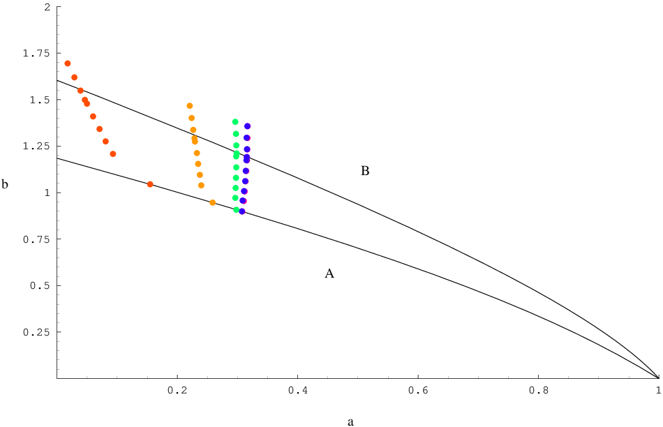
The theory in this section has three scales, the temperature , the radius of the sphere and the cutoff (which is related inversely to from the gauge/gravity duality). and are thus functions of two dimensionless quantities: and . However it can be seen from Figure (5) that the terms containing dominate over the other dimensionless quantities. For fixed , both and scale with respect to in the same way as the cutoff . This dependence on two dimensionless combinations is in contrast to the theory without the cutoff with boundary or the one with flat boundary and a cutoff. In the latter cases the free energy in gravity and hence the parameters and show much simpler dependence on the scales.
The critical exponent around the nucleation temperature, for this matrix model has been calculated in [2]. This is obtained by expanding the effective potential (4.4) in powers of . As there is no explicit dependence of the parameters on the cutoff here, the critical exponents thus remain the same. This is consistent with what we found in gravity, that the various critical exponents are insensitive to the cutoff.
We now use these above inputs to construct a model on with an infrared cutoff. This is the subject of the next section.

5 Effective model at strong coupling on with IR
Having discussed the theory on with an additional IR cutoff, let us now study its behavior as we take the radius of to infinity keeping the IR cutoff fixed. The effective theory with two parameters serves as phenomenological model for the theory on . The radius of the acts as an infrared cutoff and there is a phase transition at a temperature proportional to the inverse of the radius. As the radius of the sphere is taken to infinity the theory is always in the deconfined phase. We have seen in section (2) that for a flat boundary with an IR cutoff introduced by hand also shows the same qualitative features as the theory on the sphere. Thus at the level of a phenomenological model, it is natural to expect that (4.2) should serve as good effective model for the theory on flat space with an IR cutoff. From the point of view of the boundary theory this relies on the assumption that the effective model with IR cutoff also has an expansion in terms of the Polyakov loop. The dimensionless quantity on which the phases of the theory depend is , where is IR cutoff on the boundary. For the theory on the sphere .
The main qualitative difference as seen from section (2) is that for the flat boundary, the gravity theory with cutoff shows only one black hole solution that exists for all temperatures, whereas the theory with the boundary has two. In the latter case, the euclidean version of this unstable black hole serves as the bounce for the AdS to black hole transition. In with cutoff, one may expect a similar phenomenon when we can find an exact solution of the Einstein’s equation with an inbuilt cutoff (instead of putting it by hand). The Lorenzian version of the missing bounce would be an unstable black hole. In the appendix, we provide such a construction for the soft wall model.
From the matrix model side we have seen that it is impossible to write down a smooth potential that interpolates between two minima (corresponding to thermal AdS and the big black hole) without having an unstable maximum in between. Here in this analysis we will include this unstable maximum so that it lies in the range . The interpretation of such a saddle point is that of a stringy solution not visible in the supergravity approximation. A transition to such a string phase from the black hole phase was interpreted in [2, 9] as the gravity dual of the third order phase transition [20, 21] on the boundary. In a complete gravity solution with cutoff we expect to see an unstable black hole as mentioned in the earlier paragraph the corresponding saddle point for which in the matrix model would lie in the region .
To implement this in the following numerical analysis similar to that in section (4), we keep the unstable saddle point at . The following plots of and (Figure(7)) reflects the fact that they are functions of the dimensionless quantity .
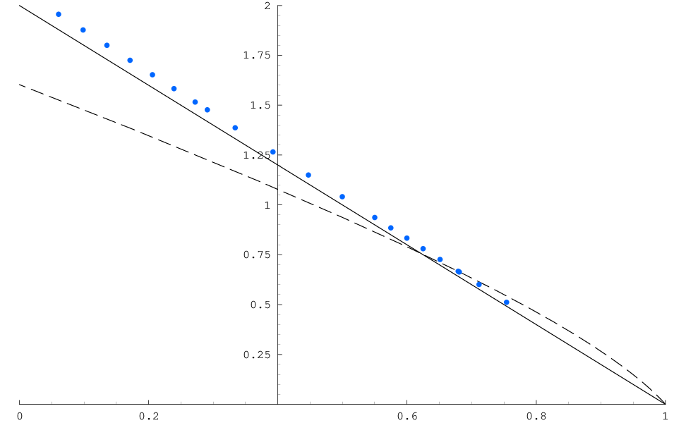
Figure (8) shows the thermal path in the space. Note that there is only one path for all values of as against Figure (6), where we have different paths for different values of . This is primarily due to the fact that here we have only one other scale, the cutoff or besides the temperature. So a change in will keep us on the same path as it can be compensated by a change in temperature. The fact that the transition temperature increases with is thus obvious as the phases depend on the dimensionless ratio . This is not so for the theory discussed in the earlier part of this section where apart from we had both and . In the numerical calculations here the critical value of is . It lies on the deconfinement line (dashed line in Figure (8)). For this value is never reached and the thermal path of always remains above the deconfinement line. For rest of the finite values of the path crosses the deconfinement line and at low enough temperatures the values of and correspond to those in the confined phase. However, since the unstable maximum is always below , the curve for all values of never crosses the third-order (black hole-string) transition line (solid line in Figure (8)) from above. The thermal history for nonzero temperature thus starts beyond this line.
6 Discussion
The analysis in this paper rests on the assumption that near the critical temperature, the effective theory governing the phase transitions for SYM on and the same on with an IR cutoff are identical. Some evidence for this assumption is obtained from the phase transitions in gravity. On the gravitational side there is no phase transition for a theory with boundary, . The theory in this case is always in one of the phases; specifically the black hole free energy is less than that of thermal AdS for all non zero temperatures. However there are two ways to get a phase transition at finite temperature; one by changing the boundary to and the other by putting a radial cutoff in gravity , that has been discussed in section (2). These result in lifting the free energy of the black hole above zero below a certain critical temperature. To this effect, the physical roles played by the cutoff and the finite radius of the three-sphere are identical. We have thus proposed that the effective matrix model (4.2) should also model the phase transitions for the theory with the cutoff. Comparing with the thermodynamic behaviour of its gravity dual, we analyzed this matrix model. This model is parametrized by two parameters and . We have numerically calculated the variations of these parameters with respect to the temperature and the cutoff. The relative behaviors of and with respect to the scales reflect those of the free energy of gravity. While for the theory on with a cutoff, due to the presence of three scales (, and ), the nature of the relative dependences is not that clear, it is quite simple when we have only two scales ( and ).
Apart from the similarities of the two configurations, there are of course certain differences that we find in the analysing the response of the matrix model parameters to changes of temperature when considering or with cutoff. For the former, the parameters are increasing functions of temperature (see [7]). This is not so in the latter case (Figure (7)). Also, from the computation of the potential for a quark-antiquark pair, we find that the potentials differ in the above two cases. These differences could be due to the details of the form of the free energy from gravity. A weak coupling computation with an IR cutoff on the gauge theory side may shed some light on the similarities and differences of the two configurations.
Acknowledgements: We would like to thank Bala Sathiapalan for discussions and for his comments on the paper. We also thank Souvik Banerjee for collaboration on results presented in the appendix. The work of TKD is supported by the South African Research Chairs Initiative of the Department of Science and Technology and National Research Foundation. Any opinion, findings and conclusions or recommendations expressed in this material are those of the authors and therefore the NRF and DST do not accept any liability with regard thereto.
Appendix A Dynamical cutoff?
In (5), we saw that it was impossible to write down a smooth potential which would interpolate between two minima (representing thermal AdS and black hole in the presence of cutoff) without having an unstable maximum. This maximum, in the gravity side, would represent a small unstable black hole which is not seen in the hard wall model of [13]. Furthermore, on generic ground, one may expect that since in this model, there is a transition from AdS to black hole, there should be a bounce solution. The Lorentzian version of this bounce would be an unstable black hole. Can the absence of such a solution in thiese models be an artifact of introducing cutoff by hand? Within the framework of soft wall model, we try to address this issue in the appendix. 33 3 This computations in this appendix was done along with Souvik Banerjee, Institute of Physics, Bhubaneswar, India.
Here, we consider a toy model in five dimensions which has a dilaton along with a non-trivial dilaton potential. This potential goes to a negative cosmological constant for small value of the scalar. We construct a family of solutions for the metric with a soft wall like behaviour of the dilaton. At large distance, the metric asymptotes to a flat AdS black hole. On the other hand, at short distance, due to dilaton backreaction, the metric gets deformed from it asymptotic structure. We indeed see that this deformation induces a small unstable black hole in the geometry. This perhaps suggests that had we dynamically intoduced a cutoff in the soft wall model of [13], a small black hole would prehaps have showed up. However, it should be noted that, we only consider a toy model and it requires a fine-tuned dilaton potential.
The model we consider is represented by the following action
| (A.1) |
We look for classical solution of this action where the metric has the following form
| (A.2) |
where are functions of only. The equations of motion can be written down by varrying the action with respect to the metric and the dilaton. They are
| (A.3) |
Here the first three equations follow from the variation of the metric and the last one is the scalar equation. Differentiating the third equation in (A.3) and using the first two, we get the last equation. In this sense, there are only three independent equations. Our will look for solutions of the above equations where the scalar depends on as
| (A.4) |
and then determine and by solving (A.3). It is easy to see that the following metric satisies the equations of motion
| (A.5) |
In the expression of the metric and are constants. The role of these constants will be discussed shortly. The potential for which (A.5) is a solution is given by
| (A.6) |
We first note that for large , as goes to zero, the potential goes to a negative constant given by
| (A.7) |
Setting
| (A.8) |
we get, asymptotically, the standard negative cosmological constant term () in the action (A.1). Furthermore, coefficient of in the potential, for , saturates the BF bound . To leading order, the metric reduces to
| (A.9) |
where we have used relation (A.8). This is an AdS black hole solution with flat horizon if we identify the mass of the black hole as
| (A.10) |
Calculating , it is easy to check that (A.5) has a curvature singularity at .
The horizon of the metric is given by the zero of . We denote the horizon radius as . It satisfies
| (A.11) |
The temperature can be computed by analysing the behaviour of the Euclidean version of the metric (A.5) near the horizon. For that, we define a new coordinate as
| (A.12) |
In terms of , (A.5) takes the form
| (A.13) |
where . This metric does not have a conical singularity at only when has a periodicity
| (A.14) |
Inverse of gives the temperature
| (A.15) |
In the limit of large ,
| (A.16) |
This is the temperature of a flat black hole in the absence of a scalar. For generic value of , the behaviour of the temperature is shown in figure (9).

We first not that the behaviour is reminiscent to that of an AdS-Schearzschild black hole with sperical horizon. The temperature has a minimum when satisfies
| (A.17) |
If we denote this value of as , we find that the minimum temperature is
| (A.18) |
Temperature is identified as the nucleation temperature where a pair of black hole nucleates. At any temperature above , there are two black holes. The smaller one is clearly unstable with negative specific heat – it’s temperature decreases as it increases in size. The bigger one, on the other hand, is always stable.
References
- [1] E. Witten, “Anti-de Sitter space, thermal phase transition, and confinement in gauge theories,” Adv. Theor. Math. Phys. 2, 505 (1998) [arXiv:hep-th/9803131].
- [2] L. Alvarez-Gaume, C. Gomez, H. Liu and S. Wadia, “Finite temperature effective action, black holes, and expansion,” Phys. Rev. D 71, 124023 (2005) [arXiv:hep-th/0502227].
- [3] B. Sundborg, “The Hagedorn transition, deconfinement and N = 4 SYM theory,” Nucl. Phys. B 573, 349 (2000) [arXiv:hep-th/9908001].
- [4] O. Aharony, J. Marsano, S. Minwalla, K. Papadodimas and M. Van Raamsdonk, “The Hagedorn / deconfinement phase transition in weakly coupled large N gauge theories,” Adv. Theor. Math. Phys. 8, 603 (2004) [arXiv:hep-th/0310285].
- [5] P. Basu and S. R. Wadia, “R-charged AdS(5) black holes and large N unitary matrix models,” Phys. Rev. D 73, 045022 (2006) [arXiv:hep-th/0506203].
- [6] P. Basu, B. Ezhuthachan and S. R. Wadia, “Plasma balls / kinks as solitons of large N confining gauge theories,” JHEP 0701, 003 (2007) [arXiv:hep-th/0610257].
- [7] T. K. Dey, S. Mukherji, S. Mukhopadhyay and S. Sarkar, “Phase Transitions in Higher Derivative Gravity,” JHEP 0704, 014 (2007) [arXiv:hep-th/0609038].
- [8] T. K. Dey, S. Mukherji, S. Mukhopadhyay and S. Sarkar, “Phase transitions in higher derivative gravity and gauge theory: R-charged black holes,” JHEP 0709, 026 (2007) [arXiv:0706.3996 [hep-th]].
- [9] L. Alvarez-Gaume, P. Basu, M. Marino and S. R. Wadia, “Blackhole / string transition for the small Schwarzschild blackhole of and critical unitary matrix models,” Eur. Phys. J. C 48, 647 (2006) [arXiv:hep-th/0605041].
- [10] I. R. Klebanov and M. J. Strassler, “Supergravity and a confining gauge theory: Duality cascades and chiSB-resolution of naked singularities,” JHEP 0008, 052 (2000) [arXiv:hep-th/0007191].
- [11] B. Sathiapalan and N. Sircar, “Can the Hagedorn Phase Transition be explained from Matrix Model for Strings?,” [arXiv:0805.0076 [hep-th]].
- [12] K. Ghoroku, A. Nakamura and M. Yahiro, Phys. Lett. B 638, 382 (2006) [arXiv:hep-ph/0605026].
- [13] C. P. Herzog, “A holographic prediction of the deconfinement temperature,” Phys. Rev. Lett. 98, 091601 (2007) [arXiv:hep-th/0608151].
- [14] R-G. Cai and J. P. Shock, “Holographic Confinement/Deconfinement Phase Transitions of AdS/QCD in Curved Spaces,” JHEP 0708, 095 (2007) [arXiv:0705.3388 [hep-th]]
- [15] J. M. Maldacena, “Wilson loops in large N field theories,” Phys. Rev. Lett. 80, 4859 (1998) [arXiv:hep-th/9803002].
- [16] S. J. Rey and J. T. Yee, “Macroscopic strings as heavy quarks in large N gauge theory and anti-de Sitter supergravity,” Eur. Phys. J. C 22, 379 (2001) [arXiv:hep-th/9803001].
- [17] O. Andreev and V. I. Zakharov, “The spatial string tension, thermal phase transition, and AdS/QCD,” Phys. Lett. B 645 (2007) 437 [arXiv:hep-ph/0607026].
- [18] H. Boschi-Filho, N. Braga and C. Ferreira, “Heavy quark potential at finite temperature from gauge/gravity duality,” Phys. Rev D74, 086001 (2006) [arXiv:hepth/0607038].
- [19] C. A. Ballon Bayona and C. N. Ferreira, “Static strings in global AdS space and quark anti-quark potential,” arXiv:0801.0305 [hep-th].
- [20] D. J. Gross and E. Witten, “Possible Third Order Phase Transition In The Large N Lattice Gauge Theory,” Phys. Rev. D 21, 446 (1980).
- [21] S. R. Wadia, “N = Infinity Phase Transition In A Class Of Exactly Soluble Model Lattice Gauge Theories,” Phys. Lett. B 93, 403 (1980).