Large curvature perturbations near horizon crossing
in single-field inflation models

This form of the inflaton potential having an unstable local maximum at the origin has been discussed many times in studies of eternal and new inflation. The main problem was to realize the initial condition for the new inflation when system starts from a top of the hill. Ten years ago the model of ”chaotic new inflation” has been proposed [6], in which the system climbs on the top during dynamical evolution of the inflaton field with initial conditions coinciding with those of chaotic inflation models. In the approach of [6] the inflation has two stages, chaotic and new, and during transition from the first stage to the second the slow-roll conditions break down (in general).

The potential has two parameters:

The inflaton starts with the rather high value of $\phi$ (we take $\phi_{\rm in}\sim 5m_{Pl}$) and rolls down to the origin. The parameter $\lambda$ is fixed by a normalization of the power spectrum on experimental data, $\lambda\sim 10^{-13}$. The evolution of the system strongly depends on the value of $v$: if $v$ is finely tuned, $\phi$ can spend some time near the origin, i.e. on the top, and then roll down to one of the two minima. In figs. 1 and 2a the time evolution for the inflaton and the parameter $\epsilon$ for the definite values of the parameters $\lambda$ , $v$ are shown. One can see that, really, $\phi\approx 0$ at some period of time and, what is important, the slow-roll approximation is invalid ($\epsilon\sim 1$) just at the time of the transition from a rolling to a temporary stay at the top of the potential.

It is well known that in situations when there is a failure of the slow-roll evolution the perturbations on super-horizon scales can be amplified and specific features in the power spectrum can arise [8, 9, 10, 11, 12] (see also the recent paper [13]). In particular, in the earliest work where this problem was studied [8], the inflation potential with a sudden gradient discontinuity leading to the power spectrum of a step-like form was considered. All this means that the predictions of the slow-roll approximation which are based on the assumption that perturbations reach an asymptotic regime outside the horizon cannot be trusted.

The curvature perturbation on comoving hypersurfaces ${\cal R}_{k}$, as a function of the conformal time $\tau$, is a solution of the differential equation (prime denotes the derivative over $\tau$)

($\phi$ is the inflaton field). The standard initial condition for this equation, corresponding to the Bunch-Davies [14] vacuum, is

where $u=z{\cal R}$. The variable $u$ had been introduced in [15, 16, 17].

The functions $\epsilon$ and $\eta$ in eq. (3) are the Hubble slow-roll parameters defined by the expressions [18]

Outside the slow-roll limit these functions are not necessarily small.

It had been demonstrated in [11] that solutions of the equation (2), at $k\ll aH$, i.e., outside horizon, are well approximated by constant if the coefficient of the friction term, $z^{\prime}/z$, doesn’t change sign near the horizon crossing. In the opposite case, if $z^{\prime}/z$ changes sign at some time, the friction term becomes a negative driving term, and one can expect strong effects on modes which left horizon near that time. In the present paper we study the corresponding features of the power spectrum, following closely the analysis of [11].

According to eq. (3), $z^{\prime}/z$ is proportional to $1+\epsilon-\eta$ and the comoving Hubble wave number $aH$. The time dependences of these functions are shown in fig. 2b. One can see that the interruption of inflation correlates with the change of the sign of $1+\epsilon-\eta$.

The time evolution of curvature perturbations for several modes is shown in fig. 3. It is clearly seen that the perturbations ${\cal R}_{k}$ for different modes freeze out at different amplitudes. The mode which crosses horizon near the moment of time when the sign of $1+\epsilon-\eta$ changes (i.e., near $t\approx 7.5m_{Pl}$) freezes at maximum amplitude, due to the exponentially growing driving term in eq. (2) (which is most effective just for this mode). It leads to the characteristic peak in the power spectrum ${\cal P}_{\cal R}(k)$,

shown in fig. 4.

The calculations of ${\cal R}_{k}$ (fig. 3) are carried out up to the end of inflation, and the power spectrum in fig. 4 also corresponds to this moment of time. We estimate approximately the reheat temperature in our case as $\sim(\lambda v^{4})^{1/4}\sim 10^{14}$ GeV. The horizon mass at the beginning of radiation era is

and maximum wave number, which equals the Hubble radius at the end of inflation, is

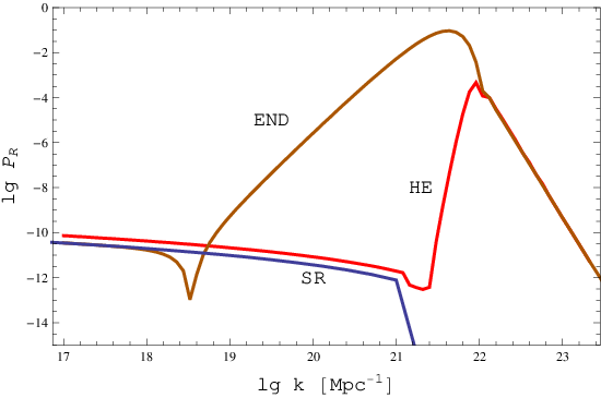
In the fig. 5 we show the power spectrum calculated for two stages of its evolution: at horizon exit (HE) and at the end of inflation (END). In the same figure the result of the calculation with an use of the slow-roll formulae is also shown. The peak of HE curve at the region of large $k$ is due to a failure (for ${\cal R}_{k}$) to reach the asymptotic limit. One can see also that the slow-roll approximation is too crude to describe perturbations at the end of inflation (this our conclusion agrees with general statements of [11]).

The Coleman-Weinberg potential has the form [19]:

It looks very similar to the previous one, but the important difference is its behavior near the origin. Namely, the CW potential behaves as $A+B\phi^{4}\ln(\phi/v)$ near the origin, i.e., it is more flat near zero, in comparison with the DW potential. Therefore, it has more e-folds of ”new inflation” [6] and, as a consequence, the peaks of the power spectrum (arising, as in the previous case, due to the temporary interruption of inflation) correspond to relatively smaller $k$ values. Besides, at the beginning of new inflation when the very flat region of the potential near zero is crossed by $\phi$, quantum fluctuations with a particle creation can be large (e.g., see below, Sec. III.3) and must be taken into account.

In fig. 6 two examples of the power spectrum calculations are shown for two different sets of parameter values. As before, the peaks are very distinct, although their amplitudes are smaller.

One can see, in particular, from fig. 4, that, in principle, the production of primordial black holes (about these objects, see original works [20, 21] and reviews [22, 23]) can be rather large in single-field inflation models with potentials of double-well type. The main conclusion is that it requires rather large fine tuning of parameters of the potential. The characteristic PBH mass is estimated by

and in the case of the spectrum of fig. 4, $M_{\rm BH}\sim 10^{7}$g. In the CW case, fig. 6, $M_{\rm BH}\sim 100M_{\odot}$ for the left peak and $M_{\rm BH}\sim 10^{27}$g for the right peak (but the amplitudes of the spectra are too small).

Recently, it has been shown [3] that inflation with CW potential is capable to produce significant number of PBHs: the parameter $v$ can be chosen (by finest tuning!) in such a way that inflaton field makes several oscillations from one minimum to another before it climbs on the top and ”new inflation” starts.

In the present paper we do not consider possibilities of a constraining of the peak amplitudes, based, for example, on the effects of PBH evaporation in early Universe (see, e.g., [24]).

We consider in more detail a case of the running mass inflation model [25, 26, 27, 28, 29, 30, 31] which predicts a spectral index with rather strong scale dependence. The potential in this case takes into account quantum corrections in the context of softly broken global supersymmetry and is given by the formula

The dependence of the inflaton mass on the renormalization scale $\phi$ is determined by the solution of the renormalization group equation (RGE).

1. The inflationary potential in supergravity theory is of the order of $M_{\rm inf}^{4}$, where $M_{\rm inf}$ is the scale of supersymmetry breaking during inflation. In turn, the mass-squared of the inflaton (and any other scalar field) in supergravity has, in general, the order of the square of Hubble expansion rate during inflation,

We suppose, for simplicity (see [25, 26, 28, 29]), that $M_{\rm inf}\sim M_{\rm s}$, where $M_{\rm s}$ is the scale of supersymmetry breaking in the vacuum,

($\tilde{m}_{s}$ is the scale of squarks and slepton masses, $\tilde{m}_{s}\sim 3$ TeV). These assumptions give the scale of the inflationary potential:

2. RGE for the inflaton mass is the following (we consider a model [28, 29] of hybrid inflation using the softly broken SUSY with gauge group $SU(N)$ and small Yukawa coupling):

$m_{0}^{2}$ and $\tilde{m}_{0}^{2}$ are, correspondingly, the inflaton and gaugino masses at $\phi=M_{P}$,

$\alpha_{0}$ is the gauge coupling constant, $\alpha_{0}=g^{2}/4\pi$. $A$ and $B$ are positive numbers of order $1$, which are different for different variants of the model, even if they are based on the same supersymmetric gauge group $SU(N)$ (it depends on a form of the superpotential, particle content of supermultiplets, etc). We use in the present parer the variant of [29] and, correspondingly, put everywhere below $A=2$ and $B=N=2$.

3. A truncated Taylor expansion of the potential around the particular scale $\phi_{0}$ (in our case, $\phi_{0}$ is the inflaton value at the epoch of horizon exit for the pivot scale $k_{0}\approx 0.002h$ Mpc^-1) is

Here, constant $c$ is defined by the equation

In turn, a Taylor expansion of eq. (15) up to linear terms gives ($t_{0}=\ln\frac{\phi_{0}}{M_{P}}$):

From eqs. (18) and (19) we obtain the expression for the constant $c$,

If $|m_{0}^{2}|\sim\tilde{m}_{0}^{2}\approx H_{I}^{2}$, then

It appears (see fig. 7b) that in our example $\phi_{0}\sim 10^{-10}M_{P}$, so, $t_{0}\sim\ln 10^{-10}\sim(-23)$. Assuming that $\alpha_{0}\sim 1/24$ (as in SUSY-GUT models), one has $\tilde{\alpha}_{0}\sim\frac{2}{2\pi}\frac{1}{24}$. In such a case, $c\sim 4\tilde{\alpha}_{0}\sim 0.06$.

If we would keep terms of higher order in $t-t_{0}=\ln\frac{\phi}{\phi_{0}}$ in the Taylor expansion of $m^{2}(t)$ in eq. (19) we would see that the real expansion parameter is $\tilde{\alpha}_{0}\ln\frac{\phi}{\phi_{0}}$ rather than $\ln\frac{\phi}{\phi_{0}}$. The smallest value of $\phi$, $\phi_{\rm end}$, in our case is $\sim 10^{-16}M_{P}$ (see fig. 7b). Even for such value of $\phi_{\rm end}$, the expansion parameter is rather small,

Having this in mind, we will use the linear approximation for the inflaton mass (eq. (19)) in the entire region of inflaton field values exploited in the present paper.

Following the previous papers, we introduce also another parameter,

where $\phi_{*}$ is the inflaton value corresponding to a maximum of the potential. This parameter connects the field value $\phi_{0}$ with the Hubble parameter during inflation and with the normalization of the CMB power spectrum:

4. The minimum value of the inflaton field which corresponds to the end of inflation can be determined from the approximate equation [29]

Using RGE, one obtains from this formula the relation

Substituting here $A=2$, $\tilde{m}_{0}^{2}=|m_{0}^{2}|=V_{0}/3M_{P}^{2}$, one has finally the approximate expression for $\phi_{\rm end}$,

which shows that the minimum field value is very sensitive to the value of the model parameter $\tilde{\alpha}_{0}$ and, in our case, does not depend on $V_{0}$. More exactly, the condition $\eta=1$ means the end of the slow-roll part of inflation. We suppose, as usual (see, e.g. [25, 26]) that in reality inflation ends by hybrid mechanism, and the critical value of inflaton field, $\phi_{\rm cr}$, is determined by the value of the Yukawa coupling $\lambda$ (in spite of the inequality $\lambda^{2}\ll\alpha$). One can check [29] that the value of $\lambda$ can always be chosen such that $\phi_{\rm cr}<\phi_{\rm end}$ and slow-roll ends before the reaching of $\phi_{\rm cr}$.

One should note that the accuracy of the approximate formula (27) is not very good. Luckily, in the approach based on the numerical calculation of the power spectrum there is no need to use it, because the value of $\phi_{\rm end}$ appears in a course of the calculation (fig. 7b).

An analysis of CMB anisotropy data [32, 33], including other types of observation [34], leads to the following main qualitative conclusions:

i) the power spectrum of scalar curvature perturbations is red, i.e., the spectral index is negative,

ii) observations are consistent, or, at least, are not in contradiction with the small positive running of the spectral index, $n_{0}^{\prime}<0.01$;

iii) the contribution of tensor perturbations in the value of the spectral index is small ($\lesssim 10^{-2}$) and, as a result, $n\approx 1+2\eta$ ; it means that $\eta$ is negative, and the potential must be concave-downward (i.e., of hill-top type), while cosmological scales cross horizon during inflation [1].

One should note that, strictly speaking, the conclusion iii) is not grounded firmly enough. According to the recent analysis [35], the present data still admit any sign of $\eta$ and $V^{\prime\prime}$.

These conclusions constrain the possible values of the parameters $s$ and $c$. Approximately, for cosmological scale one has

From the conclusion iii) it follows that $c>0$ (it is consistent with eq. (24)), from the positivity of $n_{0}^{\prime}$ (the conclusion ii) ) it follows that $s>0$. At last, the conclusion i) leads to the inequality $s<c$.

We choose for the power spectrum calculation the following values:

These numbers correspond, at cosmological scales, to the following values of slow-roll parameters:

that seems to be consistent with the present data [4].

To check the validity of the slow-roll approximation, we calculate the spectrum by the three ways: i) using the approximate analytic slow-roll formula

($\Delta N(k)\equiv\ln(k/k_{0})$; this expression is easily derived from the simplest slow-roll prediction

which gives the power spectrum to leading order in the slow-roll approximation [36]); ii) using the Stewart-Lyth approximation [37], which is valid to first order in the slow-roll approximation,

iii) by numerical integration of the differential equation for ${\cal R}_{k}$, eq. (2).

The results of the calculations are presented in figs. 7-9. Fig. 7 shows the evolution of the inflaton field $\phi$ with the scale factor and a growth of the slow-roll parameter $\eta$ with a decrease of $\phi$ from $\phi_{0}$ to $\phi_{\rm end}$. The power spectrum is shown in fig. 8 for a broad interval of comoving wave numbers. It is clearly seen that near the end of inflation, when

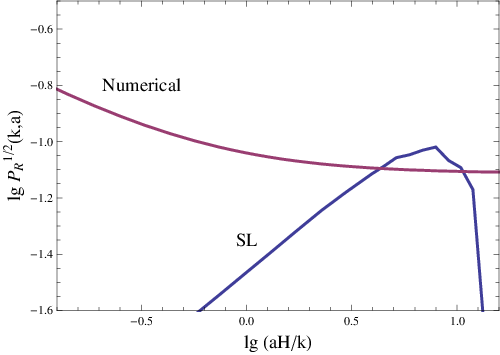
the slow-roll formulae are inaccurate: they strongly underestimate values of ${\cal P}_{\cal R}$. To illustrate this point more clearly, at the next figure we show the comparison of two curves: $aH$-dependence of the spectrum calculated numerically for a definite value of $k$, $k=10^{15.8}$ Mpc^-1, and $aH$- dependence of the Stewart-Lyth spectrum. It is seen that the numerical spectrum at the moment of crossing horizon (when $aH=k$) is already almost asymptotical, and its value distinctly exceeds the corresponding value predicted by Stewart-Lyth formula.

We calculated the curvature perturbations in terms of the classical trajectories of a scalar field associating, in particular, points in a field space with definite numbers of e-folds from the end of inflation. This description becomes incorrect if the quantum diffusion destroys the classical evolution of the field. In this case we should use the methods of stochastic inflation. The latter approach operates with the coarse-grained field, which is defined to be spatial average of the field $\phi$ over a physical volume with size larger than the Hubble radius $H^{-1}$.

In the slow-roll approximation, the evolution of the coarse-grained field $\varphi$ is governed by the first order Langevin-like equation [38, 39, 40, 41]

Here, $\xi(t)$ is a random noise field, and angular brackets mean ensemble average. The term $\frac{1}{3H}V^{\prime}(\varphi)$ describes the deterministic evolution of the field $\varphi$, in the absence of the noise term $\frac{H^{3/2}}{2\pi}\xi(t)$. The solution of eq. (36), in the absence of the noise term, is the deterministic slow-roll trajectory $\varphi_{\rm sr}(t)$. Going to finite time differences, the coefficient $\frac{H^{3/2}}{2\pi}$ can be rewritten as $\sqrt{\frac{H^{3}}{4\pi^{2}\Delta t}}$, and the evolution of $\varphi$ on timescales $\Delta t\geq H^{-1}$ can be described by a finite-difference form of the eq. (36),

The condition for the deterministic evolution is (see, e.g., [42])

Using the slow-roll connection between $V$ and $H$, one obtains

In the approach of [43] the coarse-grained field is considered as a perturbation of the classical solution $\varphi_{\rm cl}$ (which is the solution of the Langevin equation without the noise),

Here, the term $\delta\varphi_{i}(t)$ depends on the noise at the power $i$. It is assumed that the Hubble parameter in the Langevin equation depends only on the coarse-grained field $\varphi$,

Correspondingly, the Hubble parameter can be expanded perturbatively,

This approach permits to calculate the mean value of the total number of e-folds, $\langle N\rangle$, and to compare it with the corresponding ”classical” number,

Besides, one can calculate the mean value of the Gaussian probability distribution function for the coarse-grained field and to see how it behaves as a function of the current field value.

The interval of inflaton field values for which the inequality (40) holds and, therefore, the deterministic evolution dominates, is shown in fig. 10a,b. The variable $x$ in fig. 10b is defined by the relation

($\varphi_{*}$ is, as before, the point of a maximum of the potential $V(\varphi)$). It is seen from the figure that the constraints on the inflaton field following from the condition (40) are not too severe,

An accuracy of the perturbative expansion (41) for the monomial potential of stochastic inflation models was studied in [44]. Here we study this accuracy for the running mass potential, using the parameters $V_{0}$, $s$, $c$, $\varphi_{\rm end}$ introduced above. The results of the calculation of $\langle\delta\varphi_{1}^{2}\rangle$ and $\langle\delta\varphi_{2}\rangle$ are shown in fig. 11. As one can see, the perturbative expansion is good if the starting value of the inflaton field, $\varphi_{\rm in}$, is chosen to be not too close to the value of $\varphi$ at the maximum of the potential. More exactly, the parameter $x$, defined in eq. (47), must be smaller than $4\div 4.5$. The starting value $\varphi_{\rm in}$ corresponds to a beginning of the evolution, i.e., $\delta\varphi_{1}(t_{\rm in})=\delta\varphi_{2}(t_{\rm in})=0$.

If the evolution is deterministic, the correction to a classical e-fold number $N_{T}^{\rm cl}$ , given by eq. (46), is small. To estimate analytically the upper limit for this correction, we used the analytic expressions for $\langle\delta\varphi_{1}^{2}\rangle$ and $\langle\delta\varphi_{2}\rangle$ derived in [43], keeping in them leading terms only. According to these expressions, the following inequalities hold:

Using these upper limits, one can estimate the corresponding upper limits of two integrals in the expression for $\delta N_{T}$ (46). The result is the following:

It is clear from the inequalities (52) that the quantum correction to e-fold number, $\delta N_{T}$, is quantitatively small even if the value of $x$ is as large as $10$. But only if $x<4\div 4.5$ , and the perturbative expansion, eq. (41), is valid, one really can be sure that

and the evolution is deterministic.

However, this analysis is still not complete: one must check also the position of the mean value of the probability distribution function for the coarse-grained field [43]. The calculation, with taking into account the volume effects, leads to the results shown in fig. 12a,b. It is seen from the figure that in this case also, as in the calculation of the e-fold number correction, the correct choice of the initial condition plays a decisive role: there are no effects of a ”walk” of the mean value around the maximum of the potential (such effects were noticed in [43]) if evolution starts from the point which is far enough from the maximum ($x\lesssim 4.5$). Of course, the realization of the initial condition of this kind is, in itself, a problem. Supposedly, it could be provided by the previous history of eternal inflation [25, 26].