跳到论文正文
W Papers独立论文阅读器 arXiv:0806.4482 论文正文 计算阅读时间 · 0%
引用这篇论文根据当前论文元数据生成,正式投稿前建议核对。


License: arXiv.org perpetual non-exclusive license
arXiv:0806.4482v2 [gr-qc] 29 Jun 2008

Squeezed States and Affleck Dine Baryogenesis

Preprint: APS/123-QED
K. V. S. Shiv Chaitanya Email: ph03ph13@uohyd.ernet.in Affiliation: School of Physics, University of Hyderabad, Hyderabad, A.P. 500 046, India.    Bindu A Bambah Email: bbsp@uohyd.ernet.in Affiliation: School of Physics, University of Hyderabad, Hyderabad, A.P. 500 046, India.
August 24, 2026
Abstract

Quantum fluctuations in the post inflationary Affleck-Dine baryogenesis model are studied. The squeezed states formalism is used to give evolution equations for the particle and anti-particle modes in the early universe. The role of expansion and parametric amplification of the quantum fluctuations on the baryon asymmetry produced is investigated.

pacs
 98.80.Cq,98.80.Qc, 03.70.+k, 42.50.Dv

I Introduction

The dominance of matter over antimatter is known as baryon asymmetry. The generation of baryon asymmetry from an initially symmetric universe is an open problem. Baryon asymmetry is quantified by the ratio η=nbnγ\eta=\frac{n_{b}}{n_{\gamma}}, where nbn_{b} is the number of baryons and nγn_{\gamma} is the number of photons in the universe. The present value of the asymmetry in the universe is η≈10−10\eta\approx 10^{-10}. The three conditions postulated by Sakharov [1] to generate baryon asymmetry are baryon number violation, CP violation and out of equilibrium evolution of universe. Many theories have been proposed to explain baryon asymmetry. Some of them are GUT baryogenesis [2], electroweak baryogenesis [2], leptogenesis [3] and the Affleck Dine(AD) mechanism [4]. Most of these are still inadequate in explaining the value of η\eta and a lot of work remains to be done to get a complete theory of baryon asymmetry generation. In view of the inefficient baryon production in GUTS, Affleck and Dine [4] focused on the supersymmetric extension of GUTS to generate a new mechanism for baryon production based on flat directions. In the minimal supersymmetric standard model(MSSM) the number of degrees of freedom are increased by virtue of the fact that bosons and fermions have supersymmetric counterparts. The increase in the number of degrees of freedom results in directions in field space which have virtually no potential. These are known as flat directions and are made up of squarks or sleptons, so they carry baryon or lepton number. During inflation the squarks and sleptons are free to fluctuate along these directions as it costs little energy and can form condensates with a large baryon or lepton number. Supersymmetry breaking lifts these flat directions and sets a scale for the potential. Supersymmetry breaking can introduce terms that violate baryon number and CP. In the Affleck Dine model, the cosmological constant in early universe breaks the supersymmetry spontaneously during inflation and this gives rise to B−LB-L violation, satisfying Sakharov’s first condition. The scalar fields through the interaction with the inflaton field generate C and CP violation, thus satisfying Sakharov’s second condition. The expectation values of massless scalar fields can start out displaced from true minimum, oscillations around the minimum occur when the Hubble constant becomes comparable to their effective mass resulting in coherent production of scalar fields manifested as a condensate of light scalar particles. This condensate stores baryonic charge and when inflation is over its decay produces nonzero baryon asymmetry.

Dine et.al.[3]showed that baryon asymmetry can be generated for a scalar field Lagrangian with an interaction term of a general quartic type with complex couplings of the form

LI=−λ​|ϕ|4+ϵ​ϕ3​ϕ†+ϱ​ϕ4+C.C.,L_{I}=-\lambda|\phi|^{4}+\epsilon\phi^{3}\phi^{\dagger}+\varrho\phi^{4}+C.C.,

λ\lambda, ϵ\epsilon and ϱ\varrho are of the order of MS2/MG2M_{S}^{2}/M_{G}^{2}, where MGM_{G} is the grand unification scale and MsM_{s} is the supersymmetry breaking scale. The baryon number per particle at very large times (t≫mϕ−1t\gg m_{\phi}^{-1}) in both the radiation and matter dominated eras is given by

r≈I​m​(ϵ+ϱ)​ϕ02mϕ2,r\approx\frac{Im(\epsilon+\varrho)\phi_{0}^{2}}{m_{\phi}^{2}},

where, mϕm_{\phi} is of the order of MSM_{S} and ϕ0\phi_{0} is the vacuum expectation value of the scalar field. It can be seen that if ϵ\epsilon and ϱ\varrho are real then the asymmetry vanishes.

This mechanism is too efficient and produces a baryon asymmetry that is too large. Attempts to dilute this have been proposed, but most of these models use classical arguments, where additional entropy is released after baryogenesis through decay of the inflaton field [5, 6]. Other models introduce nonrenormalizable terms [7, 8]. In [9], a preliminary perturbative analysis of out of equilibrium quantum fluctuations in the AD model has been shown to lead to some amount of reduction in the asymmetry. In this paper we do a comprehensive study of quantum fluctuations in a non-perturbative fashion, using the squeezed state formalism, which allows the analysis of quantum effects and expansion on Affleck Dine baryogenesis.

II The Formalism

To carry out our analysis for AD baryogenesis for quantum fluctuations arising post inflation, we choose a Lagrangian with complex quartic couplings of the form [9]

S=∫d4​x​−g​[gμ​ν​(∂μϕ†)​(∂νϕ)−mϕ2​ϕ†​ϕ−i​λ​(ϕ4−ϕ†4)]S=\int d^{4}x\sqrt{-g}[g_{\mu\nu}(\partial^{\mu}\phi^{\dagger})(\partial^{\nu}\phi)-m_{\phi}^{2}\phi^{\dagger}\phi-i\lambda(\phi^{4}-\phi^{\dagger 4})] (1)

where ϕ\phi is a complex scalar field, mϕm_{\phi} is the mass of the scalar field and λ\lambda is a dimensionless real coupling constant. The baryon number violation comes from the coupling λ≈ϵ​MS2/MG2\lambda\approx\epsilon M_{S}^{2}/M_{G}^{2} where MSM_{S} is the supersymmetry breaking scale, ϵ\epsilon is a real parameter which characterises CP violation and MGM_{G} is the grand unification scale. The background metric is considered to be the flat FRW metric.

d​s2=d​t2−a2​(t)​d​x2ds^{2}=dt^{2}-a^{2}(t)dx^{2}

where a(t) is the expansion parameter. The classical equation of motion of the field is,

ϕ¨+3​H​ϕ˙+mϕ2​ϕ†=4​i​λ​ϕ†3\displaystyle\ddot{\phi}+3H\dot{\phi}+m^{2}_{\phi}\phi^{\dagger}=4i\lambda\phi^{\dagger 3} (2)
ϕ†¨+3​H​ϕ†˙+mϕ2​ϕ†=4​i​λ​ϕ3\displaystyle\ddot{\phi^{\dagger}}+3H\dot{\phi^{\dagger}}+m^{2}_{\phi}\phi^{\dagger}=4i\lambda\phi^{3} (3)

where H is Hubble’s constant. The initial conditions at t=t0t=t_{0} are given by

ϕ|t=t0=i​ϕ0,ϕ˙|t=t0=0.\displaystyle\phi|_{t=t_{0}}=i\phi_{0},~~~\dot{\phi}|_{t=t_{0}}=0. (4)

The baryon number per particle for large times in this model is is given by

r≈λ​ϕ02mϕ2,r\approx\frac{\lambda\phi_{0}^{2}}{m_{\phi}^{2}}, (5)

in concurrence with the classical AD result.

We now study the quantum effects on r′′{}^{\prime}r^{\prime}. We rewrite eqn.[1] in terms of conformal time η=∫d​t(a⁡(t)CLOSE\eta=\int\frac{dt}{(a(t)} as

S\displaystyle S =\displaystyle= ∫dηd3xa4[1a2((∂ϕ†∂η)(∂ϕ∂η)−(∇ϕ†)(∇ϕ))\displaystyle\int d\eta d^{3}x~a^{4}[\frac{1}{a^{2}}((\frac{\partial\phi^{\dagger}}{\partial\eta})(\frac{\partial\phi}{\partial\eta})-(\nabla\phi^{\dagger})(\nabla\phi)) (6)
−mϕ2ϕ†ϕ−iλ(ϕ4−ϕ†4)].\displaystyle-m_{\phi}^{2}\phi^{\dagger}\phi-i\lambda(\phi^{4}-\phi^{\dagger 4})].

Defining χ=a⁡(η)​ϕ\chi=a(\eta)\phi, we get

S\displaystyle S =\displaystyle= ∫dηd3x[((∂χ†∂η)(∂χ∂η)−(∇χ†)(∇χ))\displaystyle\int d\eta d^{3}x[((\frac{\partial\chi^{\dagger}}{\partial\eta})(\frac{\partial\chi}{\partial\eta})-(\nabla\chi^{\dagger})(\nabla\chi)) (7)
−(mϕ2a2−a′′a)χ†χ−iλ(χ4−χ†4)].\displaystyle-(m_{\phi}^{2}a^{2}-\frac{a^{\prime\prime}}{a})\chi^{\dagger}\chi-i\lambda(\chi^{4}-\chi^{\dagger 4})].

Decomposing χ\chi into two real scalar fields,

χ=12​(χ1+i​χ2)\displaystyle\chi=\frac{1}{\sqrt{2}}(\chi_{1}+i\chi_{2}) (8)
χ†=12​(χ1−i​χ2),\displaystyle\chi^{\dagger}=\frac{1}{\sqrt{2}}(\chi_{1}-i\chi_{2}), (9)

and substituting into the action, we get

S\displaystyle S =\displaystyle= ∫dηd3x[12(χ1′)2−12(∇χ1)2+12(χ1′)2−12(∇χ2)2\displaystyle\int d\eta d^{3}x[\frac{1}{2}(\chi^{\prime}_{1})^{2}-\frac{1}{2}(\nabla\chi_{1})^{2}+\frac{1}{2}(\chi^{\prime}_{1})^{2}-\frac{1}{2}(\nabla\chi_{2})^{2} (10)
−mη22(χ12+χ22)−2λχ1χ2[χ12−χ22]],\displaystyle-\frac{m_{\eta}^{2}}{2}(\chi_{1}^{2}+\chi_{2}^{2})-2\lambda\chi_{1}\chi_{2}[\chi_{1}^{2}-\chi_{2}^{2}]],

where prime denotes derivative with respect to conformal time η\eta and mη2=mϕ2​a2−a′′am_{\eta}^{2}=m_{\phi}^{2}a^{2}-\frac{a^{\prime\prime}}{a}.

Using the background field method to study quantum effects[10, 11, 12], we assume field χi\chi_{i}, i=1,2i=1,2, has background classical component χi​0\chi_{i0} and a quantum(order h2​π\frac{h}{2\pi}) field χ^i\widehat{\chi}_{i}:

χi=χi​0+χ^i\chi_{i}=\chi_{i0}+\widehat{\chi}_{i} (11)

where χi​0\chi_{i0} satisfies the classical equation of motion,

δ​Sδ​χi|(χi=χi​0)=0\frac{\delta S}{\delta\chi_{i}}|_{(\chi_{i}=\chi_{i0})}=0 (12)

and the field χ^i\widehat{\chi}_{i} represents quantum fluctuations around the classical solution. We expand the action in terms of Taylor series

S⁡[χi,χj]\displaystyle S[\chi_{i},\chi_{j}] =\displaystyle= S⁡[χi,χj]+δ​S​[χi,χj]δ​χi|(χi=χi​0)\displaystyle S[\chi_{i},\chi_{j}]+\frac{\delta S[\chi_{i},\chi_{j}]}{\delta\chi_{i}}|_{(\chi_{i}=\chi_{i0})} (13)
+12​(χ^i​|δ2​S​[χi,χj]δ​χi​δ​χj|(χi=χi​0)​χ^j)+…​…​…\displaystyle+\frac{1}{2}(\widehat{\chi}_{i}|\frac{\delta^{2}S[\chi_{i},\chi_{j}]}{\delta\chi_{i}\delta\chi_{j}}|_{(\chi_{i}=\chi_{i0})}\widehat{\chi}_{j})+.........

Since χi​0\chi_{i0} satisfies the classical equation of motion, the second term is zero and the contribution of the quantum fluctuations comes from the quadratic and higher order terms.

S\displaystyle S =\displaystyle= ∫dηd3x[12(χ^1′)−12(∇χ^1)2+12(χ^2′)−12(∇χ^2)2\displaystyle\int d\eta d^{3}x[\frac{1}{2}(\widehat{\chi}^{\prime}_{1})-\frac{1}{2}(\nabla\widehat{\chi}_{1})^{2}+\frac{1}{2}(\widehat{\chi}^{\prime}_{2})-\frac{1}{2}(\nabla\widehat{\chi}_{2})^{2} (14)
−mη22(χ^12+χ^22)−2λ(ρχ^1χ^2+δ(χ^12−χ^22))]\displaystyle-\frac{m_{\eta}^{2}}{2}(\widehat{\chi}_{1}^{2}+\widehat{\chi}_{2}^{2})-2\lambda(\rho\widehat{\chi}_{1}\widehat{\chi}_{2}+\delta(\widehat{\chi}_{1}^{2}-\widehat{\chi}_{2}^{2}))]

where ρ=3​(χ102−χ202)\rho=3(\chi_{10}^{2}-\chi_{20}^{2}) and δ=3​χ10​χ20\delta=3\chi_{10}\chi_{20}.

Using the Legendre transformation, we get the effective Hamiltonian of the fluctuations to be

H\displaystyle H =\displaystyle= ∫dηd3x[p^122+(∇χ^1)22+mη22χ^12+p^222+(∇χ^2)22\displaystyle\int d\eta d^{3}x[\frac{\widehat{p}_{1}^{2}}{2}+\frac{(\nabla\widehat{\chi}_{1})^{2}}{2}+\frac{m_{\eta}^{2}}{2}\widehat{\chi}_{1}^{2}+\frac{\widehat{p}_{2}^{2}}{2}+\frac{(\nabla\widehat{\chi}_{2})^{2}}{2} (15)
+mη22χ^22+2λ(ρχ^1χ^2+δ(χ^12−χ^22))]\displaystyle+\frac{m_{\eta}^{2}}{2}\widehat{\chi}_{2}^{2}+2\lambda(\rho\widehat{\chi}_{1}\widehat{\chi}_{2}+\delta(\widehat{\chi}_{1}^{2}-\widehat{\chi}_{2}^{2}))]

here p^i\widehat{p}_{i} are the canonical momenta of the χ^i\widehat{\chi}_{i} fields.

Carrying out the mode expansion of the fields, we get

χ^1=∫dk[ak†ei​k⋅x+ake−ik⋅x],\displaystyle\widehat{\chi}_{1}=\int dk[a_{k}^{\dagger}e^{ik\cdot x}+a_{k}e^{-ik\cdot x}], (16)
χ^2=∫dk[bk†ei​k⋅x+bke−ik⋅x],\displaystyle\widehat{\chi}_{2}=\int dk[b_{k}^{\dagger}e^{ik\cdot x}+b_{k}e^{-ik\cdot x}], (17)

where,

k⋅x=kμ​xμ\displaystyle k\cdot x=k_{\mu}x^{\mu} =\displaystyle= ω​η−ki​xi,\displaystyle\omega\eta-k_{i}x_{i}, (18)
d​k~\displaystyle d\tilde{k} =\displaystyle= d3​k​d​η[(2​π)3​2​ω]12,\displaystyle\frac{d^{3}kd\eta}{[(2\pi)^{3}2\omega]^{\frac{1}{2}}},
ω2\displaystyle\omega^{2} =\displaystyle= k2+mη2.\displaystyle k^{2}+m_{\eta}^{2}.

The mode Hamiltonian is

H\displaystyle H =\displaystyle= ∫d3​k(2​π)3[[ω2+λ​δ2​ω](ak†ak+a−ka−k†)\displaystyle\int\frac{d^{3}k}{(2\pi)^{3}}[[\frac{\omega}{2}+\frac{\lambda\delta}{2\omega}](a_{k}^{\dagger}a_{k}+a_{-k}a_{-k}^{\dagger}) (19)
+[ω2−λ​δ2​ω](bk†bk+b−kb−k†)]\displaystyle+[\frac{\omega}{2}-\frac{\lambda\delta}{2\omega}](b_{k}^{\dagger}b_{k}+b_{-k}b_{-k}^{\dagger})]
+(λ​ρ2​ω​(ak†​bk+a−k​b−k†+ak†​b−k†+ak​b−k)CLOSE\displaystyle+(\frac{\lambda\rho}{2\omega}(a_{k}^{\dagger}b_{k}+a_{-k}b_{-k}^{\dagger}+a_{k}^{\dagger}b^{\dagger}_{-k}+a_{k}b_{-k})
+λ​δ2​ω(ak†a−k†+aka−k)−λ​δ2​ω(bk†b−k†+bkb−k)]].\displaystyle+\frac{\lambda\delta}{2\omega}(a_{k}^{\dagger}a^{\dagger}_{-k}+a_{k}a_{-k})-\frac{\lambda\delta}{2\omega}(b_{k}^{\dagger}b^{\dagger}_{-k}+b_{k}b_{-k})]].

To see the symmetries of the Hamiltonian, we define the following generators

N1=12​(ak†​ak+a−k​a−k†),N2=12​(bk†​bk+b−k​b−k†)\displaystyle N_{1}=\frac{1}{2}(a_{k}^{\dagger}a_{k}+a_{-k}a_{-k}^{\dagger}),\;\;N_{2}=\frac{1}{2}(b_{k}^{\dagger}b_{k}+b_{-k}b_{-k}^{\dagger}) (20)
J+\displaystyle J_{+} =\displaystyle= 12​(ak†​bk+a−k†​b−k),J−=12​(bk†​ak+b−k†​a−k),\displaystyle\frac{1}{2}(a_{k}^{\dagger}b_{k}+a_{-k}^{\dagger}b_{-k}),\;J_{-}=\frac{1}{2}(b_{k}^{\dagger}a_{k}+b_{-k}^{\dagger}a_{-k}),
J0\displaystyle J_{0} =\displaystyle= 12​(N1−N2),\displaystyle\frac{1}{2}(N_{1}-N_{2}), (21)
K+=ak​b−k,K−=b−k†​ak†,K0=12​(N1+N2+1),\displaystyle K_{+}=a_{k}b_{-k},\;K_{-}=b^{\dagger}_{-k}a^{\dagger}_{k},\;K_{0}=\frac{1}{2}(N_{1}+N_{2}+1),
L1−=ak†​a−k†,L1+=a−k​ak,L10=12​(N1+1),\displaystyle L_{1-}=a^{\dagger}_{k}a^{\dagger}_{-k},\;L_{1+}=a_{-k}a_{k},\;L_{10}=\frac{1}{2}(N_{1}+1),
L2−=bk†​b−k†,L2+=b−k​bk,L20=12​(N2+1),.\displaystyle L_{2-}=b^{\dagger}_{k}b^{\dagger}_{-k},\;L_{2+}=b_{-k}b_{k},\;L_{20}=\frac{1}{2}(N_{2}+1),. (22)

We can show that (J+,J−,J0)(J_{+},J_{-},J_{0}) satisfy an s​u​(2)su(2) algebra and (K+,K−,K0)(K_{+},K_{-},K_{0}), (L1+,L1−,L10)(L_{1+},L_{1-},L_{10}), (L2+,L2−,L20)(L_{2+},L_{2-},L_{20}) satisfy s​u​(1,1)su(1,1) algebras.

In terms of these generators and the number operators , the Hamiltonian is

H\displaystyle H =\displaystyle= ∫d3​k(2​π)3[(ω2+λ​δ2​ω)N1+(ω2−λ​δ2​ω)N2\displaystyle\int\frac{d^{3}k}{(2\pi)^{3}}[(\frac{\omega}{2}+\frac{\lambda\delta}{2\omega})N_{1}+(\frac{\omega}{2}-\frac{\lambda\delta}{2\omega})N_{2} (23)
+λ​ρ2​ω​(J++J−+K++K−)\displaystyle+\frac{\lambda\rho}{2\omega}(J_{+}+J_{-}+K_{+}+K_{-})
+λ​δ2​ω(L1++L1−)−λ​δ2​ω(L2++L2−)]\displaystyle+\frac{\lambda\delta}{2\omega}(L_{1+}+L_{1-})-\frac{\lambda\delta}{2\omega}(L_{2+}+L_{2-})]

and in this form explicitly displays s​u​(1,1)su(1,1) and s​u​(2)su(2) symmetries.

We diagonalize this Hamiltonian in two steps. First we use a unitary rotation transformation and then a squeezing transformation[13]. The first transformation is given by

H1=U†​(R1)​H​U​(R1),H_{1}=U^{\dagger}(R_{1})HU(R_{1}), (24)

where

U⁡(R1)=e​x​p​[θ⁡(J+​e2​i​ξ+J−​e2​i​ξ)],U(R_{1})=exp[\theta(J_{+}e^{2i\xi}+J_{-}e^{2i\xi})], (25)

The operator U⁡(R1)U(R_{1}) provides the following transformation relations:

U†​(R1)​(akbk)​U​(R1)\displaystyle U^{{\dagger}}(R_{1})\left(\begin{array}[]{c}a_{k}\\ b_{k}\end{array}\right)U(R_{1})
=(C​o​s​(θ)e2​i​ξ​S​i​n​(θ)−e−2​i​ξ​S​i​n​(θ)C​o​s​(θ))​(akbk)\displaystyle=\left(\begin{array}[]{cc}Cos(\theta)&e^{2i\xi}Sin(\theta)\\ -e^{-2i\xi}Sin(\theta)&Cos(\theta)\\ \end{array}\right)\left(\begin{array}[]{c}a_{k}\\ b_{k}\end{array}\right)
=(AkBk),\displaystyle=\left(\begin{array}[]{c}A_{k}\\ B_{k}\end{array}\right),

the angle θ\theta is defined from the relation S​i​n​(2​θ)=(ρρ2+δ2)Sin(2\theta)=(\frac{\rho}{\sqrt{\rho^{2}+\delta^{2}}}) The creation and annihilation operators AkA_{k} and BkB_{k} are

Ak=ak​C​o​s​(θ)+bk​e2​i​ξ​S​i​n​(θ)\displaystyle A_{k}=a_{k}Cos(\theta)+b_{k}e^{2i\xi}Sin(\theta) (37)
Bk=bk​C​o​s​(θ)−ak​e2​i​ξ​S​i​n​(θ),\displaystyle B_{k}=b_{k}Cos(\theta)-a_{k}e^{2i\xi}Sin(\theta), (38)

and their complex conjugates.

The Hamiltonian H1H_{1} in terms of Ak†A_{k}^{\dagger}, Bk†B_{k}^{\dagger}, AkA_{k} and BkB_{k} is given by

H1\displaystyle H_{1} =\displaystyle= ∫ω2​d3​k(2​π)3​(m1​[Ak†​Ak+A−k†​A−k]CLOSE\displaystyle\int\omega^{2}\frac{d^{3}k}{(2\pi)^{3}}(m_{1}[A_{k}^{\dagger}A_{k}+A_{-k}^{\dagger}A_{-k}] (39)
+m2​[Bk†​Bk+B−k†​B−k]+n1​[Ak​A−k+A−k†​Ak†]\displaystyle+m_{2}[B_{k}^{\dagger}B_{k}+B_{-k}^{\dagger}B_{-k}]+n_{1}[A_{k}A_{-k}+A_{-k}^{\dagger}A_{k}^{\dagger}]
OPEN+n2​[Bk​B−k+B−k†​Bk†])\displaystyle+n_{2}[B_{k}B_{-k}+B_{-k}^{\dagger}B_{k}^{\dagger}])

where, Ω2=λ​(ρ2+δ2)\Omega^{2}=\lambda\sqrt{(\rho^{2}+\delta^{2})}, m1=ω2−Ω2ω2,m2=ω2+Ω2ω2,n1=−Ω2ω2m_{1}=\frac{\omega^{2}-\Omega^{2}}{\omega^{2}},~~m_{2}=\frac{\omega^{2}+\Omega^{2}}{\omega^{2}},~~n_{1}=-\frac{\Omega^{2}}{\omega^{2}} and n2=Ω2ω2n_{2}=\frac{\Omega^{2}}{\omega^{2}}.

We again define new generators (D1+,D1−,D10)(D_{1+},D_{1-},D_{10}), (D2+,D2−,D20)(D_{2+},D_{2-},D_{20}) satisfying s​u​(1,1)su(1,1) algebras.

D1+\displaystyle D_{1+} =\displaystyle= Ak†​A−k†,D1−=A−k​Ak,\displaystyle A^{\dagger}_{k}A^{\dagger}_{-k},\;D_{1-}=A_{-k}A_{k},
D10\displaystyle D_{10} =\displaystyle= 12​(Ak†​Ak+A−k†​A−k+1),\displaystyle\frac{1}{2}(A^{\dagger}_{k}A_{k}+A^{\dagger}_{-k}A_{-k}+1),
D2+\displaystyle D_{2+} =\displaystyle= B−k†​Bk†,D2−=Bk​B−k\displaystyle B^{\dagger}_{-k}B^{\dagger}_{k},\;D_{2-}=B_{k}B_{-k}
D20\displaystyle D_{20} =\displaystyle= 12​(B−k†​B−k+Bk†​Bk+1),\displaystyle\frac{1}{2}(B^{\dagger}_{-k}B_{-k}+B^{\dagger}_{k}B_{k}+1), (40)

and rewrite the Hamiltonian in terms of the new generators

H1\displaystyle H_{1} =\displaystyle= ∫d3​k(2​π)3ω2[[m1D10+m2D20]\displaystyle\int\frac{d^{3}k}{(2\pi)^{3}}\omega^{2}[[m_{1}D_{10}+m_{2}D_{20}] (41)
+n1[D1++D2−]+n2(D2++D1−)],\displaystyle+n_{1}[D_{1+}+D_{2-}]+n_{2}(D_{2+}+D_{1-})],

showing su(1,1) symmetry. We can diagonalize the Hamiltonian using squeezing (Bogolubov) transformation

Hf=S​(ζ2)†​S​(ζ1)†​H1​S​(ζ1)​S​(ζ2)H_{f}=S(\zeta_{2})^{\dagger}S(\zeta_{1})^{\dagger}H_{1}S(\zeta_{1})S(\zeta_{2}) (42)

where S⁡(ζ1)=e​x​p​[ζ1​D1+−ζ1∗​D1−],S⁡(ζ2)=e​x​p​[ζ2​D2+−ζ2∗​D2−]S(\zeta_{1})=exp[\zeta_{1}D_{1+}-\zeta_{1}^{*}D_{1-}],~S(\zeta_{2})=exp[\zeta_{2}D_{2+}-\zeta^{*}_{2}D_{2-}], ζ1=r1​e​x​p​[i​γ]\zeta_{1}=r_{1}exp[i\gamma] and ζ2=r2​e​x​p​[i​γ]\zeta_{2}=r_{2}exp[i\gamma].

The effect of the operators S⁡(ζ1)S(\zeta_{1}) and S⁡(ζ2)S(\zeta_{2}) on AkA_{k} and BkB_{k} is

As​(k,η)=μ1​Ak+ν1​A−k†,\displaystyle A_{s}(k,\eta)=\mu_{1}A_{k}+\nu_{1}A^{\dagger}_{-k}, (43)
As†​(k,η)=μ1∗​Ak†+ν1∗​A−k,\displaystyle A_{s}^{\dagger}(k,\eta)=\mu_{1}^{*}A_{k}^{\dagger}+\nu_{1}^{*}A_{-k}, (44)
Bs​(k,η)=μ2​B−k+ν2​Bk†,\displaystyle B_{s}(k,\eta)=\mu_{2}B_{-k}+\nu_{2}B^{\dagger}_{k}, (45)
Bs†​(k,η)=μ2∗​B−k†+ν2∗​Bk,\displaystyle B_{s}^{\dagger}(k,\eta)=\mu_{2}^{*}B_{-k}^{\dagger}+\nu_{2}^{*}B_{k}, (46)

where μ1=C​o​s​h​(r1)=m1m12−n12\mu_{1}=Cosh(r_{1})=\frac{m_{1}}{\sqrt{m_{1}^{2}-n_{1}^{2}}}, ν1=e−i​γ​S​i​n​h​(r1)=e−i​γ​n1m12−n12\nu_{1}=e^{-i\gamma}Sinh(r_{1})=e^{-i\gamma}\frac{n_{1}}{\sqrt{m_{1}^{2}-n_{1}^{2}}}, μ2=C​o​s​h​(r2)=m2m22−n22\mu_{2}=Cosh(r_{2})=\frac{m_{2}}{\sqrt{m_{2}^{2}-n_{2}^{2}}} and ν2=e−i​γ​S​i​n​h​(r2)=e−i​γ​n2m22−n22\nu_{2}=e^{-i\gamma}Sinh(r_{2})=e^{-i\gamma}\frac{n_{2}}{\sqrt{m_{2}^{2}-n_{2}^{2}}}. Thus the final diagonalized Hamiltonian after two unitary transformations is

Hf\displaystyle H_{f} =\displaystyle= ∫d3​k(2​π)3​Ω+​[As†​(k,η)​As​(k,η)+1]\displaystyle\int\frac{d^{3}k}{(2\pi)^{3}}\Omega_{+}[A^{\dagger}_{s}(k,\eta)A_{s}(k,\eta)+1] (47)
+Ω−[Bs†(k,η)Bs(k,η)+1]],\displaystyle+\Omega_{-}[B^{\dagger}_{s}(k,\eta)B_{s}(k,\eta)+1]],

where Ω+=m12−n12=ω2−2​Ω2\Omega_{+}=\sqrt{m_{1}^{2}-n_{1}^{2}}=\sqrt{\omega^{2}-2\Omega^{2}} and Ω=​m22−n22=ω2+2​Ω2\Omega_{=}\sqrt{m_{2}^{2}-n_{2}^{2}}=\sqrt{\omega^{2}+2\Omega^{2}}

The vacuum state of HfH_{f} at time η\eta is given by |0(η),0(η)>|0(\eta),0(\eta)> and vacuum state of HH at initial time is given by |0,0>|0,0>, which are related by

|0(t),0(t)>=e∫d3​k(2​π)3​[ζ1​D1+−ζ1∗​D2−]​[ζ1​D1+−ζ1∗​D2−]|0,0>|0(t),0(t)>=e^{\int\frac{d^{3}k}{(2\pi)^{3}}[\zeta_{1}D_{1+}-\zeta_{1}^{*}D_{2-}][\zeta_{1}D_{1+}-\zeta_{1}^{*}D_{2-}]}|0,0> (48)

We see that the vacuum at later times is populated with particles and anti-particles with respect to vacuum state at initial time. We can estimate the number of particles and anti-particles from the relationship between the creation and annihilation operators at initial time given by aka_{k}, and bkb_{k}, and the final creation and annihilation at later time given by operators AsA_{s} and BsB_{s}.

As​(k,η)\displaystyle A_{s}(k,\eta) =\displaystyle= (μ1​C​o​s​(θ))​ak+(ν1​S​i​n​θ​e2​i​ξ)​b−k†\displaystyle(\mu_{1}Cos(\theta))a_{k}+(\nu_{1}Sin\theta e^{2i\xi})b_{-k}^{\dagger} (49)
+(μ1​S​i​n​θ​e2​i​ξ)​bk+(ν1​C​o​s​(θ))​a−k†,\displaystyle+(\mu_{1}Sin\theta e^{2i\xi})b_{k}+(\nu_{1}Cos(\theta))a_{-k}^{\dagger},
Bs​(k,η)\displaystyle B_{s}(k,\eta) =\displaystyle= (μ2​C​o​s​(θ))​a−k+(ν2​S​i​n​θ​e−2​i​ξ)​bk†\displaystyle(\mu_{2}Cos(\theta))a_{-k}+(\nu_{2}Sin\theta e^{-2i\xi})b_{k}^{\dagger} (50)
+(μ2​S​i​n​θ​e−2​i​ξ)​b−k+(ν2​C​o​s​(θ))​ak†.\displaystyle+(\mu_{2}Sin\theta e^{-2i\xi})b_{-k}+(\nu_{2}Cos(\theta))a_{k}^{\dagger}.

The number of particles (baryons) for each mode

Nk​B​(η)=⟨Bs†​(k,η)​Bs​(k,η)⟩=|νk​2|2,N_{kB}(\eta)=\langle B_{s}^{\dagger}(k,\eta)B_{s}(k,\eta)\rangle=|\nu_{k2}|^{2}, (51)

and the number of anti-particles (anti-baryons) for each mode

Nk​B¯​(η)=⟨As†​(k,η)​As​(k,η)⟩=|νk​1|2.N_{k\overline{B}}(\eta)=\langle A_{s}^{\dagger}(k,\eta)A_{s}(k,\eta)\rangle=|\nu_{k1}|^{2}. (52)

Therefore the baryon asymmetry is

△​Nk=NB​(η)−NB¯​(η)\displaystyle\triangle N_{k}=N_{B}(\eta)-N_{\overline{B}}(\eta) =\displaystyle= Ω6ω2​(4​Ω4−ω4)\displaystyle\frac{\Omega^{6}}{\omega^{2}(4\Omega^{4}-\omega^{4})} (53)

where Ω2=λ​(ρ2+δ2)\Omega^{2}=\lambda\sqrt{(\rho^{2}+\delta^{2})}, recalling that ρ=3​(χ102−χ202)\rho=3(\chi_{10}^{2}-\chi_{20}^{2}) and δ=3​χ10​χ20\delta=3\chi_{10}\chi_{20}. We find that NB​(η)−NB¯​(η)N_{B}(\eta)-N_{\overline{B}}(\eta) is dependent on vacuum expectation values of real and imaginary parts of scalar field and coupling constant λ\lambda.

The total asymmetry is given by,

∫0∞△​Nk​d3​k\displaystyle\int_{0}^{\infty}\triangle N_{k}d^{3}k =\displaystyle= ∫0∞k2​𝑑k​Ω6ω2​(4​Ω4−ω4)\displaystyle\int_{0}^{\infty}k^{2}dk\frac{\Omega^{6}}{\omega^{2}(4\Omega^{4}-\omega^{4})} (54)
=\displaystyle= |Ω2​(mη2+2​Ω2−mη2−2​Ω2)|\displaystyle|\Omega^{2}(\sqrt{m_{\eta}^{2}+2\Omega^{2}}-\sqrt{m_{\eta}^{2}-2\Omega^{2}})|

It is interesting to see that when λ≪1\lambda\ll 1 and χ10=χ20=ϕ0\chi_{10}=\chi_{20}={\phi_{0}} the asymmetry reduces to classical value,

(NB​(η)−NB¯​(η))\displaystyle(N_{B}(\eta)-N_{\overline{B}}(\eta)) =\displaystyle= (3​λ​ϕ024​mη2)≃r.\displaystyle(\frac{3\lambda\phi_{0}^{2}}{4m_{\eta}^{2}})\simeq r. (55)

III Evolution Of Asymmetry Parameter:

In order to get some exact results and numerical values for the parameter rr after expansion, we consider a (quite realistic) expansion where we can evaluate the Bogolubov coefficients exactly.

For this consider the time evolution of wave function under the action of the Hamiltonian HfH_{f} given by (47). Going over to the coordinate representation Π(A,B)\Pi_{(A,B)} and P(ΠA,B)P_{(\Pi_{A,B})} defined by the relations [14], As​(k,η)=ei​∫Ω+​(η)​𝑑η2​Ω+​(η)​(Ω+​(η)​ΠA​(k,η)+i​PΠA​(k,η))A_{s}(k,\eta)=\frac{e^{i\int\Omega_{+}(\eta)d\eta}}{2\sqrt{\Omega_{+}(\eta)}}(\Omega_{+}(\eta)\Pi_{A}(k,\eta)+iP_{\Pi_{A}}(k,\eta)) and Bs​(k,η)=ei​∫Ω−​(η)​𝑑η2​Ω−​(η)​(Ω−​(η)​ΠB​(k,η)+i​PΠB​(k,η))B_{s}(k,\eta)=\frac{e^{i\int\Omega_{-}(\eta)d\eta}}{2\sqrt{\Omega_{-}(\eta)}}(\Omega_{-}(\eta)\Pi_{B}(k,\eta)+iP_{\Pi_{B}}(k,\eta)) ( and their complex conjugates), the Hamiltonian HfH_{f} is

Hf​(η)=∫d3​k(2​π)3​∑i=A,B12​[(Ω+)2​Πi2​(k,η)+PΠi2​(k,η)]H_{f}(\eta)=\int\frac{d^{3}k}{(2\pi)^{3}}\sum_{i=A,B}\frac{1}{2}[(\Omega_{+})^{2}\Pi^{2}_{i}(k,\eta)+P_{\Pi_{i}}^{2}(k,\eta)] (56)

The time evolution of a wave function ψ⁡(η)\psi(\eta) under the action of a Hamiltonian H⁡(η)H(\eta) is simply

H⁡(η)​ψ​(η)=i​dd​η​ψ​(η),H(\eta)\psi(\eta)=i\frac{d}{d\eta}\psi(\eta), (57)

From the form of HfH_{f} given above, it is clear that it is the direct sum of two independent Hamiltonian HA​(η)H_{A}(\eta) and HB​(η)H_{B}(\eta) for each of the AsA_{s} and BsB_{s} modes. The wave function for each momentum mode evolves as

HA​(k,η)​ψA​(k,η)=i​dd​η​ψA​(k,η),\displaystyle H_{A}(k,\eta)\psi_{A}(k,\eta)=i\frac{d}{d\eta}\psi_{A}(k,\eta), (58)
HB​(k,η)​ψB​(k,η)=i​dd​η​ψB​(k,η).\displaystyle H_{B}(k,\eta)\psi_{B}(k,\eta)=i\frac{d}{d\eta}\psi_{B}(k,\eta). (59)

Since the Hamiltonians HAH_{A} and HBH_{B} are time dependent harmonic oscillators, in the coordinate space representation the wave functions ψA​(k,η)\psi_{A}(k,\eta) and ψB​(k,η)\psi_{B}(k,\eta) can be represented by gaussian wave functions.

After some algebra, the evolution equations satisfied by the two wave functions for each mode are

ψA′′​(k,η)+Ω−2​ψA​(k,η)\displaystyle\psi^{\prime\prime}_{A}(k,\eta)+\Omega^{2}_{-}\psi_{A}(k,\eta) =\displaystyle= 0,\displaystyle 0, (60)
ψB′′​(k,η)+Ω+2​ψB​(k,η)\displaystyle\psi^{\prime\prime}_{B}(k,\eta)+\Omega^{2}_{+}\psi_{B}(k,\eta) =\displaystyle= 0.\displaystyle 0. (61)

where Ω−=k2+mϕ2​a2−a′′a−2​λ​ρ2+δ2\Omega_{-}=k^{2}+m_{\phi}^{2}a^{2}-\frac{a^{\prime\prime}}{a}-2\lambda\sqrt{\rho^{2}+\delta^{2}} and Ω+=k2+mϕ2​a2−a′′a+2​λ​ρ2+δ2\Omega_{+}=k^{2}+m_{\phi}^{2}a^{2}-\frac{a^{\prime\prime}}{a}+2\lambda\sqrt{\rho^{2}+\delta^{2}}

We rewrite these equations in the Schroedinger like form in η\eta

ψA′′+(E+V1​(a))​ψA=0,\psi_{A}^{\prime\prime}+(E+V_{1}(a))\psi_{A}=0, (62)

and

ψB′′+(E+V2​(a))​ψB=0,\psi_{B}^{\prime\prime}+(E+V_{2}(a))\psi_{B}=0, (63)

where where

E=k2+mη2\displaystyle E=k^{2}+m_{\eta}^{2} (64)
V1​(a)\displaystyle V_{1}(a) =\displaystyle= −2​λ​ρ2+δ2,\displaystyle-2\lambda\sqrt{\rho^{2}+\delta^{2}}, (65)
V2​(a)\displaystyle V_{2}(a) =\displaystyle= 2​λ​ρ2+δ2.\displaystyle 2\lambda\sqrt{\rho^{2}+\delta^{2}}. (66)

where ρ2+δ2=3​χ104+χ204−χ102​χ202\sqrt{\rho^{2}+\delta^{2}}=3\sqrt{\chi_{10}^{4}+\chi_{20}^{4}-\chi_{10}^{2}\chi_{20}^{2}}. Writing the equations in this form allows us to use the machinery of potential barrier reflection and transmission problems in quantum mechanics. The reflection (RR) and transmission (TT) coefficients can be related to the squeezing parameter (rr) through the relation s​i​n​h2​(r)=|ν|2=RTsinh^{2}(r)=|\nu|^{2}=\frac{R}{T} allowing us to calculate N(k) =|ν|2|\nu|^{2}. We can also explicitly see the origin of the asymmetry in the amplification of the particle and anti-particle modes. The particles face a potential barrier and the antiparticles a potential well. This results in a differential evolution of the particle and antiparticle modes resulting in baryon asymmetry.

We now see that there are two factors that contribute to the time evolution of the particle and anti-particle modes, the time dependence of the background classical solution and the time dependence of the expansion factor ’a⁡(η)a(\eta)’.

III.1 Slow Expansion

As a first approximation we consider the case when a′′a=0\frac{a^{\prime\prime}}{a}=0, i.e , radiation dominated universe. In this case as seen in [4] the classical equations for χ10\chi_{10} and χ20\chi_{20} are given by

χ10′′+mη2​χ10=6​λ​χ102​χ20−2​λ​χ203,\chi_{10}^{\prime\prime}+m_{\eta}^{2}\chi_{10}=6\lambda\chi_{10}^{2}\chi_{20}-2\lambda\chi_{20}^{3}, (67)

and

χ20′′+mη2​χ20=−6​λ​χ202​χ10+2​λ​χ103\chi_{20}^{\prime\prime}+m_{\eta}^{2}\chi_{20}=-6\lambda\chi_{20}^{2}\chi_{10}+2\lambda\chi_{10}^{3} (68)

To solve these equations analytically we neglect the cubic term and then we apply the boundary conditions in equation (4),to get the time dependent background solutions

χ10\displaystyle\chi_{10} =\displaystyle= λ​ϕ0(mη)3​s​i​n​(mη​η+ϵ)\displaystyle\frac{\lambda\phi_{0}}{(m_{\eta})^{3}}sin(m_{\eta}\eta+\epsilon) (69)
χ20\displaystyle\chi_{20} =\displaystyle= ϕ0mη​s​i​n​(mη​η).\displaystyle\frac{\phi_{0}}{m_{\eta}}sin(m_{\eta}\eta). (70)

Then to upto first order we have λ​ρ2+δ2=φ¯2​s​i​n2​(mη​η)\lambda\sqrt{\rho^{2}+\delta^{2}}=\overline{\varphi}^{2}sin^{2}(m_{\eta}\eta) where φ¯\overline{\varphi} is a slowly decreasing amplitude, given by φ¯2=3​λ​(ϕ0mη)2\overline{\varphi}^{2}=3\lambda(\frac{\phi_{0}}{m_{\eta}})^{2}.

The equations 62 and 63 become

ψA′′+(k2+mη2−φ¯2​s​i​n2​(mη​η))​ψA=0,\psi_{A}^{\prime\prime}+(k^{2}+m_{\eta}^{2}-\overline{\varphi}^{2}sin^{2}(m_{\eta}\eta))\psi_{A}=0, (71)

and

ψB′′+(k2+mη2+φ¯2​s​i​n2​(mη​η))​ψB=0.\psi_{B}^{\prime\prime}+(k^{2}+m_{\eta}^{2}+\overline{\varphi}^{2}sin^{2}(m_{\eta}\eta))\psi_{B}=0. (72)

.

These can be written as the Mathieu equations associated which are familiar from the parametric amplification problem in inflation.

ψA′′+ω1​k2​(1+φ¯2ω1​k2​c​o​s​(γ​η)−a′′ω1​k2​a)​ψA=0,\psi_{A}^{\prime\prime}+\omega_{1k}^{2}(1+\frac{\overline{\varphi}^{2}}{\omega_{1k}^{2}}cos(\gamma\eta)-\frac{a^{\prime\prime}}{\omega_{1k}^{2}a})\psi_{A}=0, (73)

and

ψB′′+ω2​k2​(1−φ¯2ω2​k2​c​o​s​(γ​η)+a′′ω2​k2​a)​ψB=0.\psi_{B}^{\prime\prime}+\omega_{2k}^{2}(1-\frac{\overline{\varphi}^{2}}{\omega_{2k}^{2}}cos(\gamma\eta)+\frac{a^{\prime\prime}}{\omega_{2k}^{2}a})\psi_{B}=0. (74)

. where ω1​k2=k2+mϕ2−φ¯2\omega_{1k}^{2}=k^{2}+m^{2}_{\phi}-\overline{\varphi}^{2}, ω2​k2=k2+mϕ2+φ¯2\omega_{2k}^{2}=k^{2}+m^{2}_{\phi}+\overline{\varphi}^{2} and γ=2​mη\gamma=2m_{\eta}

To solve these equations we follow the method given in [15] and [16]. From the theory of parametric resonance, the resonance is strongest if the frequency is twice ωi​k\omega_{ik}, hence we put γ=2​ωi​k+ε\gamma=2\omega_{ik}+\varepsilon with ε≪ωi​k\varepsilon\ll\omega_{ik}, the resonance condition will be satisfied if φ¯2−ε2>0\overline{\varphi}^{2}-\varepsilon^{2}>0 or |ε|<φ¯|\varepsilon|<\overline{\varphi}. We define a new variable l=εφ¯l=\frac{\varepsilon}{\overline{\varphi}} so that resonance occurs −1<l<1-1<l<1.

Then by using [16], the number of particles produced is given by

N1​k=11−l2​S​i​n​h2​(φ¯2−ε2​η),N_{1k}=\frac{1}{1-l^{2}}Sinh^{2}(\sqrt{\overline{\varphi}^{2}-\varepsilon^{2}}\eta), (75)

and the number of anti-particles is

N2​k=11−l2​S​i​n2​(φ¯2−ε2​η)\displaystyle N_{2k}=\frac{1}{1-l^{2}}Sin^{2}(\sqrt{\overline{\varphi}^{2}-\varepsilon^{2}}\eta) (76)
Refer to caption
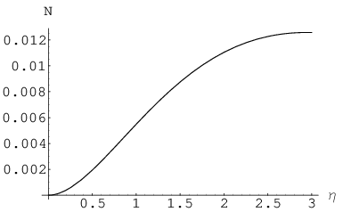
(a) (N1​(k)−N2​(k)N_{1}(k)-N_{2}(k)) and φ¯=10−2e−η/3\overline{\varphi}=10^{-2}e^{-\eta/3}
Refer to caption
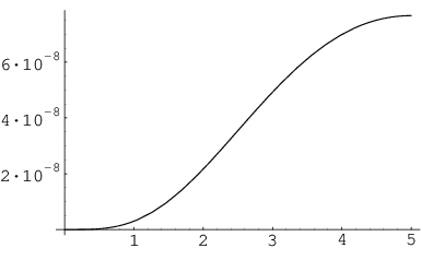
(b) (N1​(k)−N2​(k)N_{1}(k)-N_{2}(k)) and φ¯=10−3e−η/5\overline{\varphi}=10^{-3}e^{-\eta/5}

For parametric resonance, it is important that the inflaton stays in resonance band and this is possible as long as its amplitude is slowly varying function of time. The time dependence of the number of particles and antiparticles comes from the slow time variation of the decaying amplitude, which we phenomenologically approximate with φ¯2≃φ¯2e−η/τ\overline{\varphi}^{2}\simeq\overline{\varphi}^{2}e^{-\eta/\tau} where τ\tau is damping scale. In the figure (a) and (b) we have plotted N1​(k)−N2​(k)N_{1}(k)-N_{2}(k) for various values of the values of φ¯\overline{\varphi}. We can see that the value of asymmetry saturates to a finite value of ≈=10−8\approx=10^{-8}.

We assume broad resonance such that the Mathieu equation has instability bands with in which parametric resonance occurs, we shall select the first instability region as broad resonance band.

Therefore in the region of broad band resonance we replace the oscillating potential near its zeros with an asymptotically flat potential of the form

|φ¯|2​s​i​n2​(mϕ​η)≃2​|φ¯|2​t​a​n​h2​(mϕ​(η−ηi)2).\displaystyle|\overline{\varphi}|^{2}sin^{2}(m_{\phi}\eta)\simeq 2|\overline{\varphi}|^{2}tanh^{2}(m_{\phi}\frac{(\eta-\eta_{i})}{\sqrt{2}}). (77)

Then 62and 63 become

ψA′′+(k2+mϕ2−φ¯2​t​a​n​h2​(mϕ​(η−ηi)2))​ψA=0,\psi_{A}^{\prime\prime}+(k^{2}+m_{\phi}^{2}-\overline{\varphi}^{2}tanh^{2}(\frac{m_{\phi}(\eta-\eta_{i})}{\sqrt{2}}))\psi_{A}=0, (78)

and

ψB′′+(k2+mϕ2+φ¯2​t​a​n​h2​(mϕ​(η−ηi)2))​ψB=0.\psi_{B}^{\prime\prime}+(k^{2}+m_{\phi}^{2}+\overline{\varphi}^{2}tanh^{2}(\frac{m_{\phi}(\eta-\eta_{i})}{\sqrt{2}}))\psi_{B}=0. (79)

.

We get the following differential equations for the particle and antiparticle modes

d2​ψAd​y2+[κ12+φ¯2​s​e​c​h2​(y)]​ψA=0.\frac{d^{2}\psi_{A}}{dy^{2}}+\left[\kappa_{1}^{2}+\overline{\varphi}^{2}sech^{2}(y)\right]\psi_{A}=0. (80)
d2​ψBd​y2+[κ22+φ¯2​t​a​n​h2​(y)]​ψB=0.\frac{d^{2}\psi_{B}}{dy^{2}}+\left[\kappa_{2}^{2}+\overline{\varphi}^{2}tanh^{2}(y)\right]\psi_{B}=0. (81)

where

κ12\displaystyle\kappa_{1}^{2} =\displaystyle= k2−φ¯2mϕ2+1,\displaystyle\frac{k^{2}-\overline{\varphi}^{2}}{m_{\phi}^{2}}+1,
κ22\displaystyle\kappa_{2}^{2} =\displaystyle= k2mη2+1\displaystyle\frac{k^{2}}{m_{\eta}^{2}}+1 (82)
y\displaystyle y =\displaystyle= mϕ​(η−ηi).\displaystyle m_{\phi}(\eta-\eta_{i}).

Using the transmission and reflection coefficients [17], the number of particles is

n1​k=|ν1​k|2=(c​o​s2​(π​φ¯2+14))2(s​i​n​h2​(π​κ1))2,\displaystyle n_{1k}=|\nu_{1k}|^{2}=\frac{\left(cos^{2}(\pi\sqrt{\overline{\varphi}^{2}+\frac{1}{4}})\right)^{2}}{\left(sinh^{2}(\pi\kappa_{1}\right))^{2}}, (83)

the number of antiparticles is

n2​k=|ν2​k|2=(c​o​s​h​(π​φ¯2−14))2s​i​n​h2​(π​(φ¯2+κ22)).\displaystyle n_{2k}=|\nu_{2k}|^{2}=\frac{\left(cosh(\pi\sqrt{\overline{\varphi}^{2}-\frac{1}{4}})\right)^{2}}{sinh^{2}\left(\pi\sqrt{(\overline{\varphi}^{2}+\kappa_{2}^{2})}\right)}. (84)

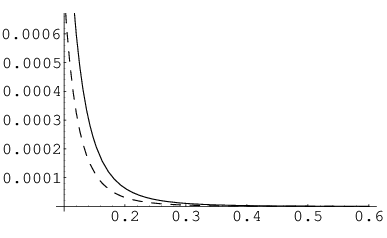
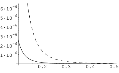
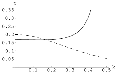
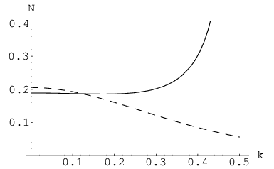
In the figure (c)and (d) the evolution of particles and antiparticles for different values of φ¯=.27\overline{\varphi}=.27 φ¯=.28\overline{\varphi}=.28, φ¯=.29\overline{\varphi}=.29 are plotted respectively. We can see clearly that the number of particles increases and number of antiparicles decreases due to differential amplification of particle and antiparicle modes.
Refer to caption
(c) N1​(k)N_{1}(k) particles(solid line) and N2​(k)N_{2}(k) and antiparticles(dash line)φ¯=.27\overline{\varphi}=.27
Refer to caption
(d) N1​(k)N_{1}(k) particles(solid line) and N2​(k)N_{2}(k) and antiparticles(dash line)φ¯=.28\overline{\varphi}=.28

III.2 Rapid Expansion

Now we consider the effect of rapid expansion on the asymmetry parameter. We consider the case when the rate of expansion dominates over the oscillation period of the classical background solution so that ρ\rho and δ\delta can be considered as time independent. We consider

a⁡(η)=(a0​η)p1−pη<η0\displaystyle a(\eta)=(a_{0}\eta)^{\frac{p}{1-p}}~~~~~~\eta<\eta_{0} (85)
a⁡(η)=C⁡(η−η0)η>η0\displaystyle a(\eta)=C(\eta-\eta_{0})~~~~~~\eta>\eta_{0} (86)

where η0=η∗−(a02​η∗)−1\eta_{0}=\eta_{*}-(a_{0}^{2}\eta_{*})^{-1}. It is convenient to set a⁡(η0)=1a(\eta_{0})=1 which sets η∗=a0−1\eta_{*}=a_{0}^{-1}, and thus η0=0\eta_{0}=0 and C=a0−1C=a_{0}^{-1} where a0=−H0a_{0}=-H_{0} for de Sitter spacetime. Here p=12\frac{1}{2} corresponds to radiation dominated universe and p→∞p\rightarrow\infty corresponds to de Sitter epoch.

Thus 62 is

d2​ψAd​η2+[k2−2​λ​ρ2+δ2−p⁡(2​p−1)(p−1)2​η2+m2H2​η2]​ψA=0\displaystyle\frac{d^{2}\psi_{A}}{d\eta^{2}}+\left[k^{2}-2\lambda\sqrt{\rho^{2}+\delta^{2}}-\frac{p(2p-1)}{(p-1)^{2}\eta^{2}}+\frac{m^{2}}{H^{2}\eta^{2}}\right]\psi_{A}=0
η<η0\displaystyle\eta<\eta_{0} (87)
d2​ψAd​η2+g1​ψA=0​η>η0\frac{d^{2}\psi_{A}}{d\eta^{2}}+g_{1}\psi_{A}=0\;\;\eta>\eta_{0} (88)

The equation 87 can be written as

d2​ψAd​τ12+[14−q2τ12+1]​ψA=0\frac{d^{2}\psi_{A}}{d\tau_{1}^{2}}+\left[\frac{\frac{1}{4}-q^{2}}{\tau_{1}^{2}}+1\right]\psi_{A}=0 (89)

where q2=(3​p−1)24​(p−1)2−mϕ2Hq^{2}=\frac{(3p-1)^{2}}{4(p-1)^{2}}-\frac{m_{\phi}^{2}}{H}, τ1=g1​η\tau_{1}=\sqrt{g_{1}}\eta and g1=k2−2​λ​ρ2+δ2g_{1}=k^{2}-2\lambda\sqrt{\rho^{2}+\delta^{2}}. the solution is given by

ψA=(g1​η)12​[Ak​Hq(1)​(g1​η)+Bk​Hq(2)​(g1​η)]\psi_{A}=(\sqrt{g_{1}}\eta)^{\frac{1}{2}}[A_{k}H_{q}^{(1)}(\sqrt{g_{1}}\eta)+B_{k}H_{q}^{(2)}(\sqrt{g_{1}}\eta)] (90)

where Hq(1)H_{q}^{(1)} and Hq(2)H_{q}^{(2)} are Hankel functions.

The solution for 88 is given by

ψA​(η>η0)=12​k​[μ​e−i​g1​η+ν​ei​g1​η]\displaystyle\psi_{A}(\eta>\eta_{0})=\frac{1}{\sqrt{2k}}[\mu e^{-i\sqrt{g_{1}}\eta}+\nu e^{i\sqrt{g_{1}}\eta}] (91)

The Bogolubov coefficients are obtained by matching the wave functions and its first derivative at η=η0\eta=\eta_{0}

The number of particles is given by.

N1​(k)=|ν1|2=4q−2​(g1a0)−2​q−1​(q−12)2​Γ2​(q).\displaystyle N_{1}(k)=|\nu_{1}|^{2}=4^{q-2}(\frac{\sqrt{g_{1}}}{a_{0}})^{-2q-1}(q-\frac{1}{2})^{2}\Gamma^{2}(q). (92)

Using similar methods for 63 the number of anti particles produced is given by

N2​(k)=|ν2|2=4q−2​(g2a0)−2​q−1​(q−12)2​Γ2​(q).\displaystyle N_{2}(k)=|\nu_{2}|^{2}=4^{q-2}(\frac{\sqrt{g_{2}}}{a_{0}})^{-2q-1}(q-\frac{1}{2})^{2}\Gamma^{2}(q). (93)

where g2=k2+2​λ​ρ2+δ2g_{2}=k^{2}+2\lambda\sqrt{\rho^{2}+\delta^{2}}, a0a_{0} is the reference scale of H0H_{0}, H0H_{0} is constant for de Sitter expansion.
Refer to caption
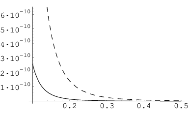
(e) (N1​(k)−N2​(k)N_{1}(k)-N_{2}(k)) q=.6q=.6 (solid line),q=.7q=.7 (dash line) here η=1\eta=1 λ=10−2\lambda=10^{-2} and ϕ0=10−2\phi_{0}=10^{-2}
Refer to caption
(f) (N1​(k)−N2​(k)N_{1}(k)-N_{2}(k)) here q=.6q=.6, η=1\eta=1 λ=10−3\lambda=10^{-3} ϕ0=10−3\phi_{0}=10^{-3}(dash line) and ϕ0=10−4\phi_{0}=10^{-4} (solid line)
Refer to caption
(g) q=.4q=.4, η=1\eta=1, φ¯=10−2\overline{\varphi}=10^{-2} and λ=10−6\lambda=10^{-6}(dash line),λ=10−7\lambda=10^{-7}(solid line)
Refer to caption
(h) (N1​(k)−N2​(k)N_{1}(k)-N_{2}(k)) here q=.4q=.4, η=1\eta=1 λ=10−3\lambda=10^{-3} ϕ0=10−3\phi_{0}=10^{-3} (solid line) and ϕ0=10−4\phi_{0}=10^{-4} (dash line)
Refer to caption
(i) q=.4q=.4, η=1\eta=1, φ¯=10−2\overline{\varphi}=10^{-2} and λ=10−6\lambda=10^{-6}(dash line),λ=10−7\lambda=10^{-7}(solid line)

First we have considered a case when p→∞p\rightarrow\infty which corresponds to de Sitter epoch.

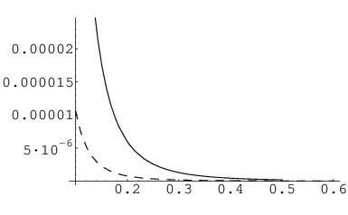
The vacuum fluctuations of massive fields on exact de Sitter background leads to density perturbations only for mϕ02H<2\frac{m_{\phi_{0}}^{2}}{H}<2 and 2<m2<9​H0242<m^{2}<\frac{9H_{0}^{2}}{4}. The corresponding characteristic values are q=0q=0, and m2H2=94\frac{m^{2}}{H^{2}}=\frac{9}{4} for de Sitter case. In the figure (e) (N1​(k)−N2​(k)N_{1}(k)-N_{2}(k)) is plotted, with q=.6q=.6 , q=.7q=.7, q=.8q=.8, which corresponds to mϕ02H<2\frac{m_{\phi_{0}}^{2}}{H}<2 for de Sitter epoch at this value the condensate starts oscillating and gives rise to fluctuations.

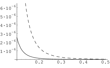
In the figure () N1​(k)−N2​(k)N_{1}(k)-N_{2}(k) is plotted for the different values of ϕ0\phi_{0} for a fixed q=.6q=.6. From the figure we can see that as the ϕ0\phi_{0} value decreases the value of asymmetry reduces. In the figure (g) N1​(k)−N2​(k)N_{1}(k)-N_{2}(k) is plotted for the different values of λ\lambda for a fixed q=.6q=.6 and ϕ0\phi_{0}. From the figure we can see that as the λ\lambda value decreases the value of asymmetry reduces. Large occupation number in a given mode means that quasi-particles formed a condensate. Therefore from the figure we can see that once the quantum fluctuations are switched on the value of asymmetry reduces but does not goes to zero.

Now we consider the case when p→12p\rightarrow\frac{1}{2} which corresponds to radiation dominated universe.

In the radiation dominated universe, when mϕ02H<.25\frac{m_{\phi_{0}}^{2}}{H}<.25, then only the vacuum fluctuations of massive fields will be switched on, and the characteristic values for q=0q=0, is m2H2=14\frac{m^{2}}{H^{2}}=\frac{1}{4} .

In the figure (h) N1​(k)−N2​(k)N_{1}(k)-N_{2}(k) is plotted for the different values of ϕ0\phi_{0} for a fixed q=.4q=.4. corresponds to mϕ02H=.16\frac{m_{\phi_{0}}^{2}}{H}=.16. From the figure we can see that once the quantum fluctuations are switched on the value of asymmetry reduces. In the figure (i) N1​(k)−N2​(k)N_{1}(k)-N_{2}(k) is plotted for the different values of ϕ0\phi_{0} for a fixed q=.4q=.4 for quantum fluctuations, in this case the asymmetry goes to 10−3​λ​ϕ02mϕ210^{-3}\frac{\lambda\phi_{0}^{2}}{m^{2}_{\phi}}. We conclude that the Affleck Dine mechaniam when combined with the CP violating amplifacation of vacuum flucutations during inflation can give an acceptable value of baryon asymmetry of universe.

IV Conclusion

In this paper we have studied the non-equilibrium quantum effects of Affleck Dine baryogenesis in the post inflationary scenario. In the paper [9] they have studied the model using the nonequilibrium dynamics and used perturbative methods to get the asymmetry, whereas the methodology developed here using squeezed states or Bogolubov transformations has allowed us to derive the general evolution equations for baryon and anti-baryon modes non-perturbatively in an expanding FRW metric. In our evolution equation the effective potential is dependent upon the expansion parameter a⁡(η)a(\eta) and inflaton potential. The amount of particle production in the de Sitter expansion is calculated as the tunnelling through a barrier of potential V⁡(a)V(a). We find that by considering different inflationary scenarios and parametric resonance we can control the asymmetry parameter ”r” to a much lower value than in the classical Affleck Dine model. Of course, we have used a simplified toy model, but the method is general and can work for a more realistic scenario also.

Baryon asymmetry remains an intriguiging unsolved issue in physics. In view of the standard model being in sufficient to explain this essential fact about the universe, one has to look beyond the standard model. Supersymmetry is a compelling idea beyond standard model. Hence finding arguments for baryon asymmetry in MSSM is a natural idea. The Affleck Dine mechanism which uses the flat directions in supersymmetric models is therefore a very promising mechanism for baryon asymmetry generation. Furthermore there is also very compelling evidence that universe went through an inflationary phase and particles were generated by reheating processes. Thus combining the two we should be able to get a plausible and viable scenario for baryon asymmetry. Means to reduce the rather over efficient generation of baryon asymmetry in Affleck Dine mechanism require a th0rough study. In this paper we have done a systematic study of the effects of inflation and parametric amplification of quantum fluctuations on the baryon asymmetry generated in post-inflationary Affleck Dine baryogenesis. Since a variant of the Affleck Dine mechanism is also used to account for dark matter as well as in most exotic scenarios of baryogenesis our method should be useful in this context also.

Acknowledgements.
This work was supported by SAP/CAS, U.G.C and as well as Revised fellowship scheme, U.G.C. KVSSC and BAB thank Prof C. Mukku for his valuable comments on this paper.

References

  • [1] A. Sakharov, Eksp. Tero. Fiz. 5, 32 (1967).
  • [2] A. D. Dolgov, eprint hep-ph/9707419.
  • [3] M. Dine and A. Kusenko, Reviews of Modren Physics. 76, 1 (2004).
  • [4] I. Affleck and M. Dine, Nuclear Physics B. 249, 361 (2004).
  • [5] A. D. Linde, Phys Letts B 160, 243 (1985).
  • [6] J. Ellis, Phys Letts B 191, 343 (1987).
  • [7] K. W. Ng, Nucl Phys B 321, 528 (1989).
  • [8] M. Dine, L. Randall, and S. Thomas, Nucl Phys B 458, 291 (1996).
  • [9] Y.-Y. Charng, D.-S. Lee, C. N. Leung, and K.-W. Ng, Phys. Rev D. 72, 123517 (2005).
  • [10] B. A. Bambah and C. Mukku, Annals of Physics 314, 54 (2004a).
  • [11] B. A. Bambah and C. Mukku, Phys. Rev D. 70, 034001 (2004b).
  • [12] B. A. Bambah and C. Mukku, eprint hep-th/0307286.
  • [13] A. M. Perelomov, Generalized Coherent States and their Applications (Springer-Verlag, Berlin, 1986).
  • [14] B. A. Bambah, K. V. S. S. Chaitanya, and C. Mukku, Annals of Physics. 322, 849 (2007).
  • [15] L. D. Landau and E. Lifshitz, Corse of Theoretical Physics Volume 1, (Pergamon Press, New York, 1960).
  • [16] D. I. Kaiser, Phys. Rev D. 53, 1776 (1996).
  • [17] S. Flugge, Practical Quantum Mechanics,Vol.I and Vol.II, (Springer, New York, 1976).