Plane symmetric thin-shell wormholes: solutions and stability

The planar black hole or a black membrane metric is given by [34, 35, 36, 37]

where $\alpha$ is the inverse of the characteristic length of the system, which here we adopt as given by the negative cosmological constant, i.e., we put $\alpha^{2}=-\Lambda/3$. The ranges of $t$ and $r$ are $-\infty<t<+\infty$ and $0\leq r<+\infty$. The range of the coordinates $x$ and $y$ determine the topology of the plane symmetric metric. For the planar case, the topology of the two-dimensional space, $t={\rm constant}$ and $r={\rm constant}$, is $R^{2}$, with coordinate range $-\infty<x<+\infty$ and $-\infty<y<+\infty$. For the cylindrical case the topology is $R\times S^{1}$, with $-\infty<x<+\infty$ and $0\leq\alpha\,y<2\pi$. For the toroidal case the topology is $S^{1}\times S^{1}$ (i.e., the torus $T\,^{2}$), with $0\leq\alpha\,x<2\pi$ and $0\leq\alpha\,y<2\pi$. A scalar polynomial singularity occurs at $r=0$, which can be demonstrated through the Weyl scalar, given by $C^{{\mu}{\nu}{\alpha}{\beta}}C_{{\mu}{\nu}{\alpha}{\beta}}={12M^{2}}/{(\alpha^{2}\,r^{6})}$, where Greek indices are spacetime indices, $\mu=t,r,x,y$. It can also be found through the Kretschmann scalar, given by $R^{{\mu}{\nu}{\alpha}{\beta}}R_{{\mu}{\nu}{\alpha}{\beta}}=24\alpha^{4}+12{M^{2}}/{(\alpha^{2}\,r^{6})}$, but since the first term is innocuous, the Weyl scalar suffices. In particular, we shall consider the planar topology case, and the analysis considered in this work applies equally well for solutions with toroidal and cylindrical topologies. Note that considering a positive value for $M$, an event horizon occurs at $r_{h}=M^{1/3}/\alpha$, consequently resulting in a planar black hole solution, or black membrane. Considering a negative value for $M$, we verify that no event horizons occur, implying the existence of a singular naked membrane. A remark is in order here: cylindrically thin-shell wormholes were analyzed in [19], which are different to the planar, cylindrical or toroidal topological solutions we analyze, as for our case infinity carries the same topology as the throat

An interesting wormhole solution consists in applying the cut-and-paste construction. We consider two copies of the black membrane or planar black hole solution, Eq. (1), removing from each spacetime the four-dimensional regions described by

where $a$ is a constant. The condition $a>M^{1/3}/\alpha$ is important to avoid the presence of an event horizon. The removal of these two regions results in two manifolds, geodesically incomplete, with boundaries given by the following timelike hypersurfaces

We now identify these two timelike hypersurfaces, $\partial\Omega^{+}=\partial\Omega^{-}\equiv\partial\Omega$, which results in a manifold, now geodesically complete, with two regions connected by a wormhole. The throat of the wormhole, i.e., the junction surface, is situated at $\partial\Omega$, and may be viewed as behaving like a domain wall connecting two universes. One can then write the intrinsic metric to $\partial\Omega$ as

where $\tau$ is the proper time on $\partial\Omega$.

In general terms, the position of the junction surface is given by $x^{\mu}(\tau,x,y)$, and the respective $4$-velocity is

where $\tau$ is the proper time on the surface. We shall use the Darmois-Israel formalism to determine the surface stresses at the junction boundary [11]. The intrinsic surface stress-energy tensor, $S_{ij}$, is given by the Lanczos equations in the form $S^{i}_{\;j}=-\frac{1}{8\pi}\,(\kappa^{i}_{\;\,j}-\delta^{i}_{\;j}\kappa^{k}_{\;\,k})$, where Latin indices are intrinsic surface indices which run through $i=\tau,x,y$. For notational convenience, the discontinuity in the second fundamental form or extrinsic curvatures is given by $\kappa_{ij}=K_{ij}^{+}-K_{ij}^{-}$. The second fundamental form is defined as

where $n_{\gamma}$ is the unit $4$-normal to $\partial\Omega$, and the superscripts $\pm$ correspond to the exterior and interior spacetimes, respectively. The parametric equation for $\partial\Omega$ is given by $f(x^{\mu}(\xi^{i}))=0$. The unit $4$-normal to $\partial\Omega$ is given by

with $n^{\mu}\,n_{\mu}=+1$.

Applying to our particular case, the position of the junction surface is given by $x^{\mu}(\tau,x,y)=(t(\tau),a(\tau),x,y)$, and the respective $4$-velocity is

where the overdot denotes a derivative with respect to $\tau$, which is defined as the proper time on $\partial\Omega$. The unit normal to the junction surface may be determined by Eq. (7) or by the contractions, $u^{\mu}n_{\mu}=0$ and $n^{\mu}n_{\mu}=+1$, and is given by

Considerable simplifications occur due to plane symmetry, namely $\kappa^{i}_{\;j}={\rm diag}\left(\kappa^{\tau}_{\;\,\tau},\kappa^{x}_{\;\,x},\kappa^{x}_{\;\,x}\right)$. Thus, the surface stress-energy tensor may be written in terms of the surface energy density, $\sigma$, and the surface pressure, ${\cal P}$, as $S^{i}_{\;j}={\rm diag}(-\sigma,{\cal P},{\cal P})$, which taking into account the Lanczos equations, reduce to

This simplifies the determination of the surface stress-energy tensor to that of the calculation of the non-trivial components of the extrinsic curvature, or the second fundamental form. Therefore, taking into account the metric of Eq. (1) and the definition of the second fundamental form, Eq. (6), we have

From Eqs. (10)-(11), we deduce the surface stress-energy components given by

respectively. Obviously $\sigma$ and $\cal P$ obey the conservation equation

In order to be able to solve the two nontrivial equations (14)-(15) for $\sigma(\tau)$ and $a(\tau)$, one needs to specify an equation of state. Here we impose a cold equation of state

which follows if the temperature is zero, $T=0$, in a general equation of state of the form ${\cal P}={\cal P}(\Sigma,T)$, $\sigma=\sigma(\Sigma,T)$, where $\Sigma$ is the baryonic mass density. In our study we will make the analysis initially with a generic cold equation of state of the form (17), i.e., without invoking any specific equation of state, see [14], and then particularizing to a specific cold equation of state, see [3].

Besides doing the analysis for a general equation of state of the form ${\cal P}={\cal P}(\sigma)$, as in Eq. (17), we want to study specific cases by giving an equation of state. We resort in the following to a particularly interesting equation of state, namely, an equation of state analogous to the dark energy equation of state considered in cosmology, i.e.,

Such a dark energy fluid can be divided into three cases: a normal dark energy fluid when $-1<\omega<0$, a cosmological constant fluid when $\omega=-1$, and a phantom energy fluid when $\omega<-1$. All of these fluids are possible candidates responsible for the accelerated expansion of the Universe. But in addition to its cosmological interest, the equation of state (18) can also be used for domain walls and wormholes, connecting opposite spacetime regions.

The case of a static wormhole is particularly simple, yet it provides interestingly enough results. Equations (14)-(15) reduce to

Since there is a generic equation of state of the type given in Eq. (17), the constants $M$, $a$, and $\alpha$ are inter-related.

The surface energy density in (19) is negative, implying the violation of the weak and dominant energy conditions. The surface pressure is always positive. The null energy condition is verified if $\sigma+{\cal P}>0$ is satisfied. Thus, taking into account the relationship

we see that the null energy condition is verified only for $M>0$, and violated for $M<0$. The strong energy condition is satisfied if $\sigma+{\cal P}>0$ and $\sigma+2{\cal P}>0$, and by continuity implies the null energy condition. Using the condition

we verify that the strong energy condition is readily satisfied for $M>0$.

It is also of interest to analyze the attractive or repulsive character [28] of this plane symmetric traversable wormhole. The four-velocity of a static observer is $u^{\mu}=dx^{\mu}/{d\tau}=(u^{\,t},0,0,0)=(1/\sqrt{\alpha^{2}r^{2}-M/\alpha r}\,,0,0,0)$. The observer’s four-acceleration is $a^{\mu}=u^{\mu}{}_{;\nu}\,u^{\nu}$, so that taking into account Eq. (1), the only non-zero component is given by

From the geodesic equation, a radially moving test particle which starts from rest initially has the equation of motion

Therefore, $a^{r}$ is the radial component of proper acceleration that an observer must maintain in order to remain at rest at constant $(r,x,y)$. It is interesting to note that a wormhole is “attractive” if $a^{r}>0$, i.e., observers must maintain an outward-directed radial acceleration to keep from being pulled into the wormhole; and “repulsive” if $a^{r}<0$, i.e., observers must maintain an inward-directed radial acceleration to avoid being pushed away from the wormhole. Note that for $M>0$, the wormhole is attractive. For $M<0$, the wormhole is repulsive for the values $r<\sqrt[3]{|M|/2}/\alpha$, and attractive for $r>\sqrt[3]{|M|/2}/\alpha$. In particular, for $r=\sqrt[3]{|M|/2}/\alpha$ static observers are geodesic.

To justify the equation of state (18) let us first try a well known case, the surface stress-energy tensor without trace. As we will show now, this is no good. The traceless surface stress-energy tensor, $S^{i}_{\;\,i}=0$, i.e., $-\sigma+2{\cal P}=0$, could be a case of particular interest, since the Casimir effect with a massless field gives a stress-energy tensor of this type. This effect is theoretically invoked to provide exotic matter to the system considered at hand. From $-\sigma+2{\cal P}=0$ we deduce $\alpha^{2}a^{2}=M/(2\alpha a)$, which is inside the event horizon of the planar black hole, or the black membrane, and so is no good. As in the spherical symmetric case [3], there is no solution of the Einstein field equations because $\sigma$ and ${\cal P}$ are imaginary, as one may readily verify from Eqs. (19)-(20). So, one has to resort to the equation of state given in (18), i.e., ${\cal P}=\omega\sigma$, with $\omega<0$. That $\omega$ has to be less than zero can be seen directly from equations (19)-(20). Indeed, as the surface energy density is always negative, $\sigma<0$, and the tangential surface pressure is always positive, ${\cal P}>0$, then the equation of state (18) imposes the condition $\omega<0$, i.e., a dark energy equation of state. As mentioned above, one can subdivide the $\omega<0$ fluid further into a normal dark energy fluid ($-1<\omega<0$), a cosmological constant fluid ($\omega=-1$), and a phantom energy fluid ($\omega<-1$) This type of dark energy fluids are considered in cosmology, as well as in domain wall and wormhole building. Indeed, for the latter, the particular case of $\omega=-1$ reduces to $\sigma+{\cal P}=0$, which corresponds to the classical membrane, this being described by the three-dimensional generalization of the Nambu-Goto action, and being the simplest domain wall one may construct [3]. From Eq. (21), one finds that this case is only valid when $M=0$, thus from Eqs. (19)-(20) the surface energy density and surface pressure are given by $\sigma=-{\cal P}=-\frac{\alpha}{2\pi}$. Another interesting example, is when $\omega<-1$, where it has been shown that spherically symmetric traversable wormholes can be theoretically supported by phantom energy [29, 30].

Now, using Eqs. (19)-(20), we obtain the following relationship

where

Note that if $M>0$ then $\omega$ has the range $-\infty<\omega<-1$ and $-1/4<\omega<0$. One should impose the additional no horizon condition, $M<\alpha^{3}a^{3}$, since if the condition is not satisfied there are no static solutions, and moreover the wormholes would be inside their own gravitational radius, a situation which is of no interest here. Thus, imposing the additional no horizon condition one gets from Eq. (25) that $\Gamma(\omega)<1$, which means the $M>0$ case is restricted to $-\infty<\omega<-1$. If $M=0$, i.e., the fluid is the spacetime background fluid with a negative cosmological constant, it naturally gives the corresponding equation of state, i.e., $\omega=-1$. If $M<0$ then $\omega$ is restricted to the range $-1<\omega<-1/4$. Thus the full range of $\omega$ is $-\infty<\omega<-1/4$, see Fig. 1.

To analyze the dynamics of the wormhole, we consider that the throat is a function of the proper time, as measured by an observer comoving with the throat [3, 14, 13]. Assume that the position of the throat is given by $x^{\mu}(\tau,x,y)=(t(\tau),a(\tau),x,y)$. As mentioned, Eqs. (14)-(15) imply the energy conservation equation (16), which in turn can be put in the form

Equation (27) may also be rewritten as

Taking into account an equation of state of the form given in Eq. (17), i.e., ${\cal P}={\cal P}(\sigma)$, Eq. (28), can be integrated to yield

This result may be formally inverted to provide $\sigma=\sigma(a)$. Equation (14) may be recast into the following form

which may also be written as $\dot{a}^{2}=-V(a)$, where the potential is defined as

We sketch an analysis of this potential by dividing it into three cases. (i) When $(2\pi\sigma(a))^{2}>\alpha^{2}$, from Eq. (30), we can divide into two cases $M\geq 0$ and $M<0$. For $M\geq 0$ we verify that the wormhole is dynamically unstable. Depending on the initial conditions, this wormhole solution will either collapse to $a=0$ or explode to $a\rightarrow\infty$. For $M<0$ the wormhole never collapses, and depending on the form of $\sigma(a)$ it may or may not explode. Thus, for $M<0$ the solution may be stable. (ii) When $(2\pi\sigma(a))^{2}=\alpha^{2}$, then Eq. (30) reduces to $\dot{a}^{2}-M/\alpha a=0$. Thus, we can divide also into two cases $M\geq 0$ and $M<0$ For $M\geq 0$ the differential equation has the following solutions $a(\tau)=\frac{\alpha}{4M}\left(\pm 12M^{2}\alpha^{-2}\tau\mp 12M^{2}\alpha^{-2}C\right)^{2/3}\,,$ where $C$ is a constant related to the initial radius of the wormhole, $C=\frac{2}{3}\sqrt{\alpha a_{0}^{3}/M}$. We verify that if $\tau\rightarrow\infty$, the wormhole explodes, $a\rightarrow\infty$. The wormhole collapses to $a\rightarrow 0$ in the proper time $\tau=C$. In addition to $(2\pi\sigma)^{2}=\alpha^{2}$, considering $M=0$, we have a stable and static wormhole solution, i.e., $\dot{a}(\tau)=0$, as we verified whilst analyzing the classical membrane in static wormholes. For $M<0$ there is no solution. (iii) When $(2\pi\sigma(a))^{2}<\alpha^{2}$, for $M\geq 0$ one has that the wormhole will not explode, but will collapse. For $M<0$ there is no solution.

Before entering the analysis for the specific dark energy equation of state (18), we give a simple example of a dynamically stable solution with a specific choice for the matter field surface energy density. Note that to be dynamically stable, the potential is required to be bounded from above and from below. To achieve this, one may consider the following specific choice for the surface energy density $\sigma(a)=\pm\frac{1}{2\pi}\left\{\alpha^{2}-\frac{1}{a^{2}}\left[k_{1}(a-k_{2})^{2}-k_{3}+\frac{M}{\alpha a}\right]\right\}\,,$ where $k_{i}>0$ (with $i=1,2,3$) are constants. Substituting this expression in Eq. (31), provides the following potential $V(a)=k_{1}(a-k_{2})^{2}-k_{3}\,,$ which can easily be depicted qualitatively. The zeroes of $V(a)$ are situated at $a_{1,2}=k_{2}\mp\sqrt{k_{3}/k_{1}}$, where the lower root $a_{1}=k_{2}-\sqrt{k_{3}/k_{1}}$ is required to obey $a_{1}>M^{1/3}/\alpha$, in order to avoid a black hole solution.

Considering the equation of state given in Eq. (18), i.e., ${\cal P}=\omega\sigma$, from Eq. (29), we deduce

where $a_{0}$ is the initial position of the throat and $\sigma_{0}=\sigma(a_{0})$. The qualitative behavior is transparent from Fig. 2. As $\omega\rightarrow 0$ and for high values of $\alpha=a/a_{0}$, then $\sigma\rightarrow 0$. On the other hand for decreasing values of the parameter $\omega$ and for high $\alpha=a/a_{0}$, then $\sigma\rightarrow-\infty$. For $\omega\rightarrow 0$ and $\alpha=a/a_{0}\rightarrow 0$, then $\sigma\rightarrow-\infty$. Note that considering the equation of state of the domain wall [3, 15], $\sigma+{\cal P}=0$, from Eq. (27) we have $\dot{\sigma}=0$, i.e., $\sigma={\rm const}<0$.

Relative to the stability analysis, by substituting Eq. (32) into the potential, Eq. (31), yields the following relationship

where the following definitions were considered for notational simplicity

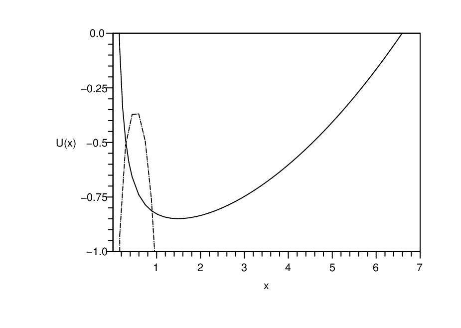
with $\bar{\sigma}_{0}=2\pi\sigma_{0}$. A stability analysis is depicted in Fig. 3 for specific numerical values, which may be considered as representative for the present stability analysis. For positive values of $\bar{M}$, depicted by the dashed curve, we have considered the specific values of $\bar{M}=0.15$, $\omega=-3/2$ and $\bar{\alpha}=0.15$. One verifies that for this case, the wormhole is unstable. For $\bar{M}<0$, depicted by the solid curve, we have considered the specific numerical values of $\bar{M}=-0.15$, $\omega=-1/2$ and $\bar{\alpha}=0.15$, and one verifies the stability of the wormhole.

Thus, in summary, for $\bar{M}>0$, one sees that the wormholes are unstable, as depicted by the dashed curve in Fig. 3. For $\bar{M}=0$, not depicted, the wormhole is static and neutrally stable. For $\bar{M}<0$, which is depicted by the solid curve in Fig. 3, the wormhole is stable against expansion and collapse, it will oscillate between a maximum value and a minimum value of $a$.

An alternative to the partial stability analysis of Section III.1 is to consider a linear perturbation around a static solution with radius $a_{0}$. The respective static values of the surface energy density and the surface pressure are given by Eqs. (19)-(20). To know whether the equilibrium solution is stable or not, one must analyze the shell’s equation of motion near the equilibrium solution. This means that in order to solve this equation one has to know the equation of state of the shell’s matter.

In this subsection, rather than choosing a specific equation of state, we shall follow the Poisson-Visser reasoning [14], and put quite generally ${\cal P}={\cal P}(\sigma)$, see (17). Thus, the potential given by Eq. (31), may be rewritten as

Linearizing around the stable solution at $a_{0}$, a second order expansion of $V(a)$ around $a_{0}$ provides

where the prime denotes a derivative with respect to $a$. To determine $V^{\prime}(a)$ and $V^{\prime\prime}(a)$, it is useful to rewrite the conservation of the surface stress-energy tensor, Eq. (27), as $\sigma^{\prime}a=-2(\sigma+{\cal P})$, taking into account $\sigma^{\prime}=\dot{\sigma}/\dot{a}$. Defining the parameter $\eta(\sigma)$ by

and since ${\cal P}(\sigma)^{\prime}=(d{\cal P}/d\sigma)\sigma^{\prime}=\eta\sigma^{\prime}$, we have $\sigma^{\prime}+2{\cal P}^{\prime}=\sigma^{\prime}(1+2\eta)$. Thus, $V^{\prime}(a)$ and $V^{\prime\prime}(a)$, are given by

respectively. Evaluated at the static solution, using Eqs. (19)-(20), and taking into account Eqs. (21)-(22), we find $V(a_{0})=0$ and $V^{\prime}(a_{0})=0$, with $V^{\prime\prime}(a_{0})$ given by

where $\eta_{0}=\eta(\sigma_{0})$. For this, note that Eq. (40) may be expressed as

by taking into account the surface stresses evaluated at the static solution $a_{0}$, given by Eqs. (19)-(20). The potential $V(a)$, Eq. (36), is reduced to

so that the equation of motion for the wormhole throat presents the following form

to the order of the approximation considered. The solution is stable if and only if $V^{\prime\prime}(a_{0})>0$. Three cases may be distinguished, namely, $0<{M}/{(\alpha a_{0})^{3}}<1$ (which essentially amounts to $M>0$), ${M}/{(\alpha a_{0})^{3}}=0$ (which essentially amounts to $M=0$), and ${M}/{(\alpha a_{0})^{3}}<0$ (which essentially amounts to $M<0$). For $0<{M}/{(\alpha a_{0})^{3}}<1$, the solution is stable if

For the specific case of ${M}/{(\alpha a_{0})^{3}}=0$ we have a static and neutrally stable wormhole solution. This can be readily verified from Eq. (41), which implies $V^{\prime\prime}(a_{0})=0$, and consequently $\dot{a}=0$, from Eq. (43). Thus any $\eta_{0}$ is possible, i.e.,

Note that this is consistent with the analysis outlined in Sections III.1.2 and III.2.1. For ${M}/{(\alpha a_{0})^{3}}<0$, the stability region is dictated by the following inequality

The stability regions are plotted in Figure 4.

One can put Eqs. (44)-(46) in terms of the matter fields. These yield,

respectively.

It is also interesting to consider the stability regions, using the linearization approach, for the specific case of the dark energy equation of state, ${\cal P}=\omega\sigma$, (see Eq. (18)). By considering ${\cal P}=\omega\sigma$, we note that for this linear equation of state, we have $\eta_{0}=\omega$. Now, using the stability condition $V^{\prime\prime}(a_{0})>0$, from Eqs. (49)-(47) we have the following stability conditions. For $M>0$, one has to take into account the relation between $\omega$ and the mass $M$ given in Eq. (25) (see also Fig. 1), i.e., if $M>0$ then $\omega$ is in the range $\omega<-1$, whereas the range $\omega>-\frac{1}{4}$ is physically unacceptable since it violates the no horizon condition. So, for $M>0$, $\omega$ is in the range $\omega<-1$, and the solutions are unstable. For $M=0$ one has $\omega=-1$, and the solution is stable. For $M<0$, $\omega$ is in the range $-1<\omega<-1/4$, and the solutions are stable. Thus, we finally have

respectively. So, thin shell wormholes made of phantom energy ($\omega<-1$, $M>0$) are unstable, while thin shell wormholes made of dark energy fluid ($-1<\omega<-1/4$, $M<0$) or of cosmological constant fluid ($\omega=-1$, $M=0$) are stable.