Exact solution of a stochastic SIR model
Abstract
The susceptible-infectious-recovered (SIR) model describes the evolution of three species of individuals which are subject to an infection and recovery mechanism. A susceptible can become infectious with an infection rate by an infectious - type provided that both are in contact. The - type may recover with a rate and from then on stay immune. Due to the coupling between the different individuals, the model is nonlinear and out of equilibrium. We adopt a stochastic individual-based description where individuals are represented by nodes of a graph and contact is defined by the links of the graph. Mapping the underlying Master equation into a quantum formulation in terms of spin operators, the hierarchy of evolution equations can be solved exactly for arbitrary initial conditions on a linear chain. In case of uncorrelated random initial conditions the exact time evolution for all three individuals of the SIR model is given analytically. Depending on the initial conditions and reaction rates and , the -population may increase initially before decaying to zero. Due to fluctuations, isolated regions of susceptible individuals evolve and unlike in the standard mean-field SIR model one observes a finite stationary distribution of the -type even for large population size. The exact results for the ensemble averaged population size are compared with simulations for single realizations of the process and also with standard mean field theory which is expected to be valid on large fully-connected graphs.
pacs
05.70.Ln, 05.50.+q, 64.60.Ht, 75.10.Hk, 05.70.FhI Introduction
Infections produce further infections. This observation has long inspired theoreticians to find simple tractable evolution equations to model such a situation. One traditional and rather simple approach is the so-called SIR model originally introduced in [1], see also [2] and [3]. Here a certain population is divided into three distinct classes: the susceptible, , wherein the individual is healthy but is allowed to catch the disease; further there are the infectious, denoted as which is infected and can transmit the disease and the recovered which is immune to further infection [4]
Although the model is quite simple, it captures important features of the temporal dynamics of an infection cycle. In so far the model is appropriate to describe a well-localized disease outburst. Due to the coupling of the three different groups and the process is non-linear. Furthermore, as long as there is an infectious population the system is in an nonequilibrium state not characterized by any physical a priory principle such as detailed balance. Despite its simplicity the SIR-model has not been solved exactly if fluctuations, which inevitably occur in a real system, are included in its description. In this paper we present such an exact solution using a mapping of the underlying Master equation into a quantum formulation. There appears a whole hierarchy of evolution equations for certain expectation values which can be closed and from which among other things the exact time evolution of the expected population size for each class can be extracted analytically in closed form.
Our effort can be grouped in the permanent attraction exerted by modern biology and social science to understand the evolution of cooperative behavior. It is well known that in unstructured populations, natural selection favors defectors over cooperators. For that problem we also need the insight provided by mathematical tools. The SIR model offers a simple approach by a set of evolution equations [3, 5, 6, 7, 8, 9, 10]. To discuss the spreading of epidemics the SIR model can be implemented on a network [11], which is further discussed in [13, 12, 14, 15]. The general scheme and the properties of networks are elaborated in detail [16]. In such a network approach, individuals are represented by nodes which are in either of the three states . Contact between individual is modelled by links between the nodes. For maximal connectivity, where each individual is in contact with every other, i.e. for the fully connected graph, one expects the deterministic standard mean field equations for the SIR model to be valid for large population size even if the infection and recovery are stochastic. In contrast, fluctuations are expected to cause substantial deviations from the mean field behaviour if the connectivity is low. Hence it is highly desirable to study the opposite case of minimal connectivity as realized in a linear chain. In the present paper we analyze the SIR model on a linear chain based upon the master equation [18] which is reformulated in terms of second quantized operators [19, 20, 21, 22]. The method enables us to apply the algebraic properties of spin operators to determine a closed set of evolution equations for higher-order cluster functions. These cluster functions describe groups of susceptibles which can be infected from the boundary of the region. The time evolution for the cluster functions can be closed which makes the problem exactly solvable. This allows for a quantitative comparison with the mean-field solution as given by the deterministic standard SIR model and also with the random behavior of single realizations of the process obtained from Monte-Carlo simulation.
The paper is organized as follows. In Sec. 2 we first define the standard deterministic SIR model and then introduce the stochastic dynamics that we consider to account for fluctuations. In Sec. 3 we describe the mathematical apparatus required for obtaining the exact results. This section can be skipped by readers not interested in the mathematical details. For an introduction into the quantum approach used there we refer to the reviews [20, 21]. In Sec. 4 we present the exact results for the expected population densities and compare them with analytical results from the mean-field approach. In Sec. 5 we discuss results of Monte-Carlo simulations for single realizations of the process . In Sec. 6 we finish with some conclusions.
II Stochastic SIR model on a graph
Let us denote with and the number of susceptibles, infectious and recovered individuals. The total number is conserved
| (1) |
In the traditional treatment of the SIR model the population strength is treated as a real number and infection and recovery are governed by the nonlinear set of coupled equations
| (2) |
The first equation describes the decrease of the susceptible population through the infection of a susceptible individual by an infectious one. The loss is proportional to the infection rate and since by definition and are non-negative, the loss is monotone. The second equation describes the gain of the infectious population of individuals by infection of susceptibles as described in the first equation and the spontaneous recovery with rate . The last equation follows simply from the conservation of the total number of individuals.
These equations describe a deterministic evolution for each population class which entirely neglects fluctuations and which offers no description of the state of an individual member of the entire population. These equations may be regarded as a mean-field treatment of some fluctuating random process and therefore we shall refer to this standard SIR model as mean field SIR model. In view of our further approach it is appropriate to introduce the population densities where stands for one of three classes . Obviously the densities satisfy .
We now define a stochastic SIR dynamics that describes the state of each individual. This description allows for randomness and hence fluctuations in both the infection and recovery process. In our individual-based version of the model the individuals are represented by the nodes of a graph. For each node we introduce state variables which specify the state of the node. For reasons that become clear below we represent these state variables as occupation numbers which take value 0 or 1 as follows: If node is in the susceptible state at time , we say that . If node is in the infectious or recovered state then . Likewise we define occupation numbers which by definition are subject to the constraint . With this definition we define the (random) population sizes of class of individuals
| (3) |
where the sum is taken over all nodes of the graph. Considering nodes ensures a strict conservation law analogous to (1) for the deterministic SIR model. Contact between two individuals is represented by a link between two nodes. This defines the graph.
The stochastic dynamics of the model is realized by the following Markov process. A susceptible individual at a node becomes infectious after an exponentially distributed random time with rate where
| (4) |
is the total number of infectious individuals which are in contact with at time . This quantity is an integer random variable that depends on the current state of the system. On the other hand, an infectious individual at node recovers after an exponentially distributed random time with fixed rate . Once an individual is recovered it remains so. All infection and recovery processes occur independently of each other.
Thus this stochastic process is in double contrast to the evolution studied in the mean-field approach. There recovery and infection are deterministic and the infection rate is proportional to the size of the full population of infectious individuals. The latter property is recovered in our individual-based approach if each individual is in contact with every other, i.e., if the underlying network is the complete graph of nodes. If then in addition the population size is send to infinity, one expects fluctuations to disappear by the law of large numbers. Hence the traditional SIR model as described by (2) may be regarded as a deterministic limit of the evolution of our stochastic process on a complete graph in the thermodynamic limit of infinite population size.
In our stochastic model the main quantity of interest is the expected state of a node at time , given some initial distribution. We shall focus on uncorrelated random initial distributions with some given mean population size for infectious and susceptible individuals. In this case the expectation value is independent of the node and we write it in slight abuse of notation and [23]. Moreover, in order to quantify and highlight the possible effect of fluctuations due to incomplete connectivity between individuals we study the most “non-mean-field” setting possible. I.e. we consider the lowest possible connectivity between individuals which is realized in a periodic chain of nodes. The dynamics of the model is then realized by the following transitions on neighboring nodes
| (5) |
The first two processes mean that a single susceptible can catch the disease when it is in contact with infectious individuals situated on the neighboring nodes. The last process in Eq. (5) characterizes the recovering process, where an infectious individual recovers and becomes immunized, independently of the state of other individuals.
III Quantum Approach to Nonequilibrium Systems
III.1 Master equation in a quantum Hamiltonian representation
Since the combined influence of noise and spatial degrees of freedom is an important issue in a theoretical understanding of biological and ecological processes [17] the dynamics due to Eq. (5) is formulated in a master equation for the full probability distribution of the process. Here we use a very transparent method, the transformation of the master equation into a quantum language. This exact mapping enables us to get an exact solution for the process defined above. Since the method borrows techniques from condensed matter and particle physics, we use well-established jargon that is slightly different from that above. In particular, we shall refer to nodes of the graph as sites on a lattice, and to the state variable as occupation numbers by particles of type .
Let us summarize briefly the most important steps, for a detailed account of the approach see [20, 21]. The master equation for the joint probability reads
| (6) |
Here stands for a certain configuration of and particles at time . In a lattice gas description each lattice point is either empty or single occupied leading to for each type. Using the expansion
| (7) |
Eq. (6) can be rewritten as an equivalent equation in a Fock-space
| (8) |
where the operator is determined in such a manner that its matrix elements correspond to those of . The formal solution of that equation is
| (9) |
This expression gives the probability distribution at time in terms of the initial distribution at time .
It should be emphasized that the procedure is up to now independent of the realization of the basic vectors . As shown by Doi [19] the average of an arbitrary physical quantity can be calculated by the average of the corresponding diagonal operator
| (10) |
with the summation vector . The evolution equation for an operator can be cast in a commutator relation which reads
| (11) |
As the result of the procedure, all the dynamical equations governing the
classical problem are determined by the structure of the evolution operator
and the commutation rules of the operators.
The evolution operator for the process defined by Eq. (5) reads
| (12) | |||||
Here and are the annihilation and creation operators for and types. The operators and represent the particle number operators with the eigenvalues and . The particle number operator corresponds to the occupation variable and corresponds to .
The meaning of the evolution operator defined in Eq. (12) is now transparent: The first term on the right hand side describes the annihilation of a susceptible at site and a simultaneous creation of an infectious at the same site provided the neighboring lattice site is occupied by an infectious indicated by the number operator . Mathematically this property is manifest in the commutator relation
| (13) |
and similar rules for the and . The operators commute at different lattice sites and the anticommute at the same lattice site. The anticommutator rule implies the exclusion principle, i.e. the eigenvalues of the particle operators are restricted to and therefore the corresponding averages fulfills . Similar relations hold for . From the definition follows
| (14) | |||||
| (15) |
and correspondingly
| (16) |
for the probability of finding node in the recovered state. Notice that these expectation values imply a double average over the initial distribution and over realizations of the stochastic dynamics.
III.2 Cluster functions
These equations involve second-order correlators which hints at the non-linear nature of the problem. To analyze the situation let us further study the higher order correlators appearing in Eqs. (17). For illustration we present the result for the two-point correlator
| (18) |
To make a more systematic approach let us define the -point cluster functions
| (19) |
Obviously these functions are zero if one of the sites inside of the cluster is recovered with probability 1. Furthermore the functions and are sensitive to the fact that a cluster of susceptible individuals is diminished by infection at the border of the cluster. The introduction of these cluster functions is the decisive trick of our treatment which makes the nonlinear problem solvable.
The cluster equations simplify under the natural assumption of a translation invariant initial distribution. Then one can drop the -dependence and after a straightforward calculation only taking into account the algebraic properties Eq. (13) we end up with the following set of coupled equations for the cluster functions
| (20) |
For non-translation invariant distributions the evolution equations for the cluster functions still close, but retain an extra -dependence. The meaning of the evolution equations is immediately visible. The cluster described by decreases by infecting node with rate and recovery of node with rate . Furthermore the cluster grows by increasing its length from to through infection of node . The exact evolution equation of the -cluster can be made plausible in similar terms. This competition between growth and reduction processes of the clusters yields a non-trivial steady state of the process discussed below.
The second cluster equation can be solved recursively by treating the term as an inhomogeneity of the remaining homogeneous first-order linear ordinary differential equation. One obtains
| (21) |
where is an arbitrary initial condition.
Inserting that solution in the first equation we find in a similar fashion the solution
| (22) | |||||
These results are exact for arbitrary translation invariant initial distributions. For uncorrelated random initial distribution of each class of individuals the initial conditions for the cluster functions read
| (23) |
Here the initial densities of infectious and susceptible individuals are and . Inserting this in Eq. (21) and Eq. (22) results in
| (24) | |||||
| (25) |
where the relaxation time is defined by
| (26) |
We draw attention to the fact that the relaxation time depends on the initial conditions through the initial density of susceptibles. This is a consequence of the highly non-ergodic and far-from-equilibrium nature of the process. Both cluster functions decay monotonically in time to zero.
IV Exact solution
Using the exact result for the cluster expectation values for random initial conditions obtained in the previous section from the quantum approach, we are now in a position to obtain the exact time evolution for the expected number of individuals of each class. In terms of the cluster functions and the evolution equations for the quantities
| (27) |
read
| (28) |
Notice that is strictly positive for all finite times. Hence the density of susceptible individuals is strictly monotonically decreasing which follows from the fact that no susceptibles are generated in the process.
The averaged number of susceptible person at time follows immediately from Eqs. (24), leading to
| (29) | |||||
The decay of the susceptible persons is not purely Arrhenius-like but given by a superposition of two relaxation times.
In the long time limit we find a nonzero stationary solution
| (30) |
which can be written in the more transparent form
| (31) |
which makes the dependence on initial conditions and the recovery/infection ratio fully explicit.
In the same manner we find the expected density of infectious persons
| (32) |
with
| (33) |
Due to Eq. (1) is the expected density of recovered individuals.
For a comparison with the predictions of the original SIR model defined by the set of differential equations (2) the mean-field solution we highlight some features of this mean field model. From the first equation in Eq. (2) we conclude that is a monotonically decreasing function. Moreover, the last equation implies that the stationary value for the infectious class is . Both properties are shared by our stochastic SIR model. In the condition for the existence of a maximum in the number of infectious individual, the situation is more subtle. Writing the second equation in Eq. (2) in the form
| (34) |
one realizes that a maximum occurs if . It is reached at a time where . Inserting this into the first equation one may write in terms of the normalized population densities . Interestingly, the exact relation (28) asserts that in our stochastic model the maximum occurs at a time determined by the same relation in the case of random initial conditions. Hence, our model reproduces several key features of the original SIR model. For these features, the low connectivity and stochasticity are unimportant for a comparison of average behavior of the stochastic dynamics with the deterministic behavior of the mean field model. Notice though, that the actual value of is not the same in the two models. It is also interesting to observe that the mean field expression for can be written in terms of the concentration in the form , i.e. the maximum in occurs at a time where an initial concentration of susceptibles of order 1 has almost disappeared and only a finite total number (of order 1) of susceptibles are left in the population. This is in contrast to our stochastic model where the maximum in occurs at a concentration of susceptibles which is of order 1. In this respect, the mean field model fails to capture the effects of low connectivity.
For a more detailed analysis of the mean field SIR model we introduce which due to the first equation in Eq. (2) satisfies . Differentiating again and using the second equation gives an integrable second order equation for . After one integration one obtains
| (35) |
where is an integration constant. In case of the initial conditions and it results . Combining the last relation for with Eq. (2) we then find the relation
| (36) |
In the same manner we find
| (37) |
where obeys
| (38) |
It corresponds to an overdamped motion in a potential
| (39) |
This equation of motion does not allow for a closed solution in terms of elementary functions.
In the limit Eq. (36) gives a transcendental equation for the stationary population of susceptibles
| (40) |
This has no solution in closed form, but for large one obtains
| (41) |
which decays exponentially in the population size . This result is strongly different from the exact solution (31) where one finds a finite stationary value of order 1 even for infinite .
As a final remark we point out that in the mean field approximation one decomposes higher order correlators according to . Identifying with the density of susceptibles and correspondingly we get from (28) mean field equations of the form (2), but with an infection rate . Hence the mean field approximation of our stochastic model yields a deterministic SIR dynamics with renormalized infection rate .
V Monte Carlo simulation data
Our exact results are obtained for the thermodynamic limit of infinite population size, and they are results for a statistical ensemble of processes, averaged both over random initial states and histories. Here we present Monte Carlo simulation results for single runs of the process which demonstrate that even if the moderate population size is moderate, fluctuations around the computed expectation value are rather small. This mean that the computed expectation values represent the typical behavior that one expects in a single outbreak of the disease. Only for very small populations the fluctuations around the expected mean become significant.
We have performed the numerical simulation of the problem as follows. Initially, each site is occupied independently and randomly by a susceptible with probability and by an infectious individual with probability . For the dynamics we have chosen a random sequential update algorithm as follows. An arbitrary lattice site is chosen randomly. If this site is occupied with an infectious , then the -state decays to with probability . If it does not decay, then with equal probability 1/2 an adjacent site on the left or right hand site is chosen. If the chosen neighboring site is occupied by a susceptible , then is converted into with probability . If lattice site is occupied by a susceptible or the site is recovered nothing happens. Then a new site is selected randomly and the procedure is repeated. such update steps then define one Monte-Carlo time step. We remark that for an efficient implementation of the process one may keep a list of coordinates of infectious sites and select sites only from this list. However, for population sizes of the order of such optimization is irrelevant for the study of single realizations of the process.
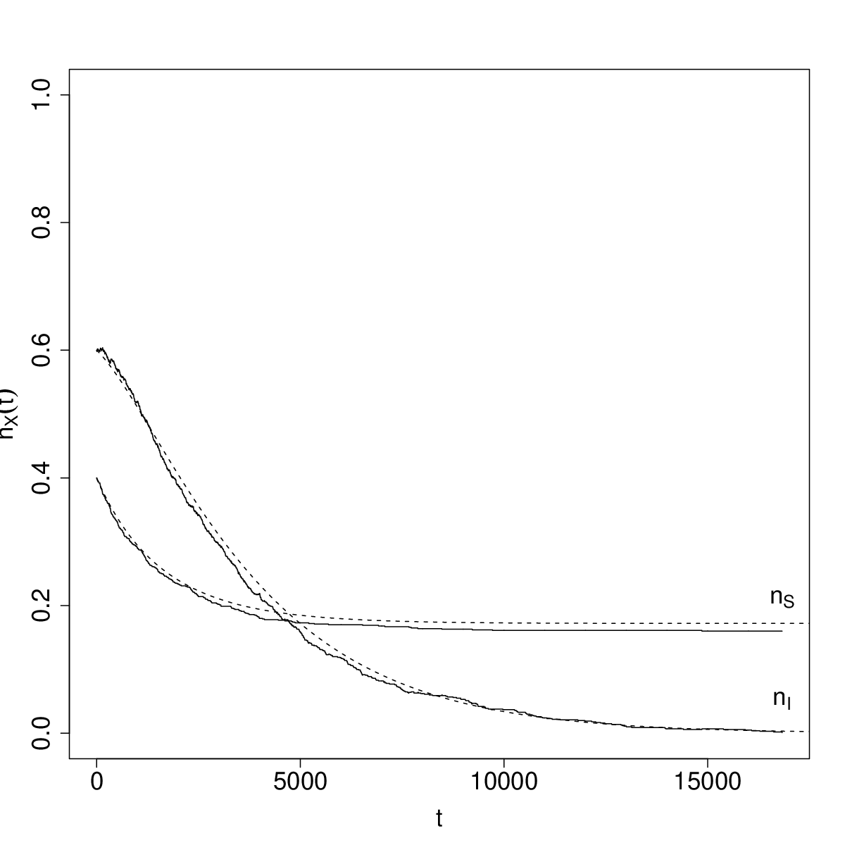
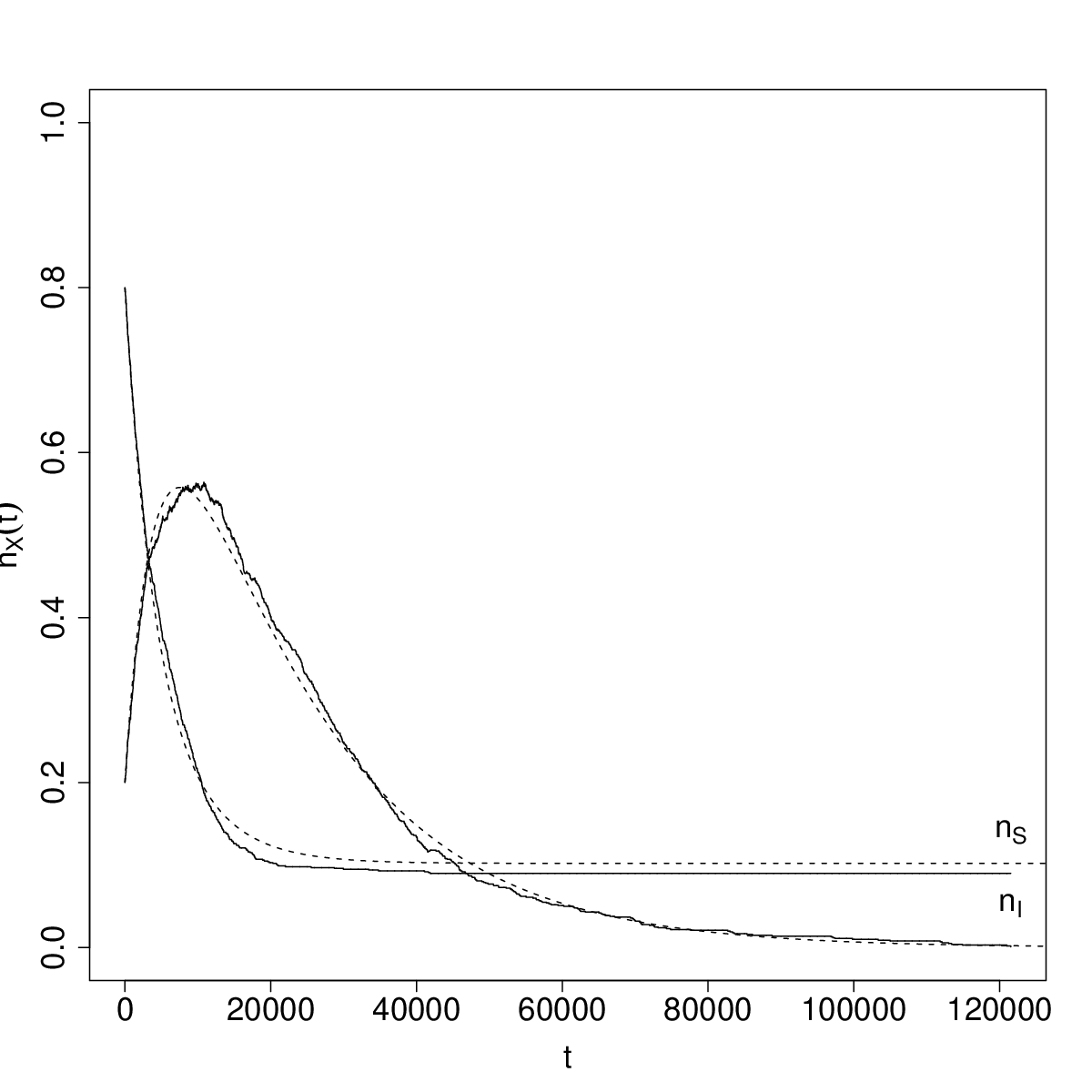
In Fig. 1 we show simulation data for two different runs with population size 1000, demonstrating the absence (Fig. 1(a)) or presence (Fig. 1(b)) respectively of a maximum in the number of infectious particles. The maximum occurs at values of which is of order 1, rather than as predicted by mean field theory. The finite limiting value of the susceptible population density is also clearly seen. The corresponding mean field value would be nearly zero. For a comparison of this single run with the computed mean values the corresponding exact expressions (29) and are shown as well. The deviations are at most in the range of a few percent. (32).
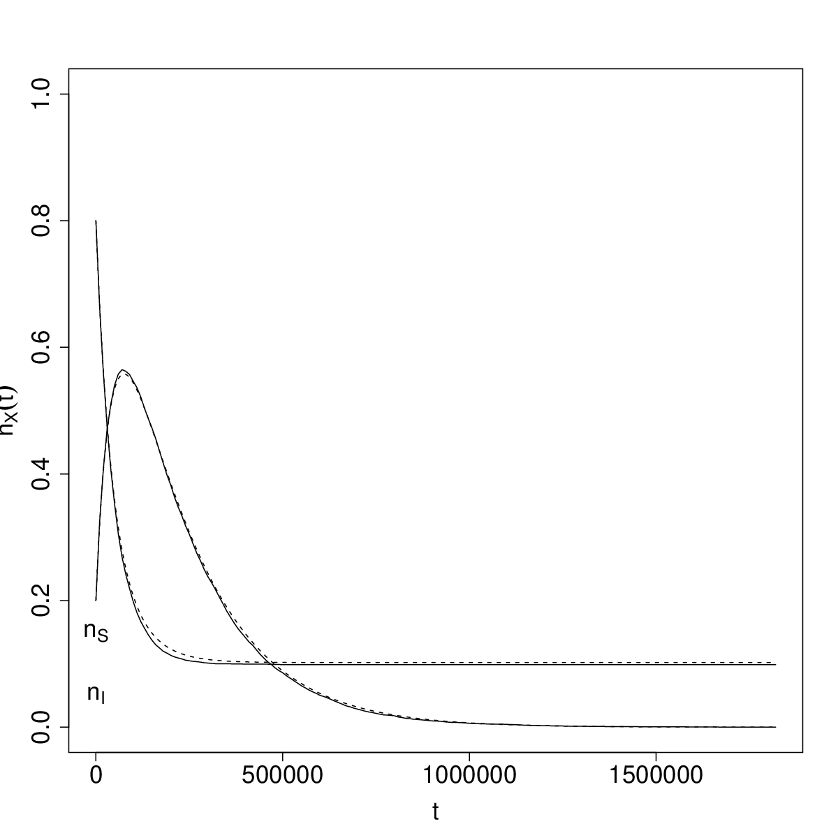
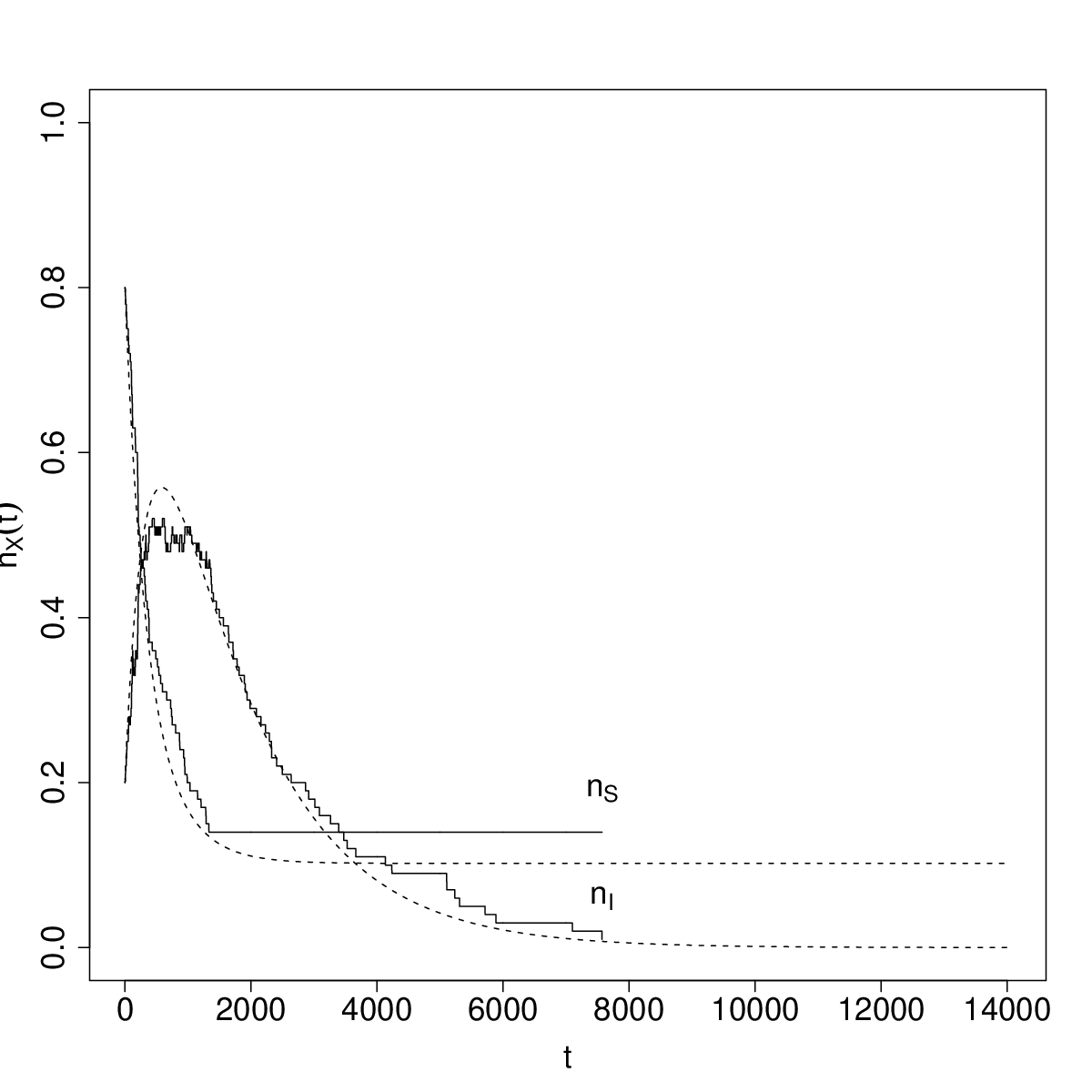
In Fig. 2 we show simulation data and the exact solution for different total number of individuals. Fig. 2 demonstrates the he increasing effect of fluctuations for small population sizes. For population sizes of the order of fluctuations become irrelevant.
VI Conclusions
In this work we have analyzed a SIR model for a population of susceptible , infectious and recovered individuals evolving under a stochastic dynamics. In order to study the effect of fluctuations due to incomplete contact between the individuals we have defined the model on a linear chain. As an appropriate tool we have considered the master equation for the probability density which we wrote in a quantum formulation in terms of second quantized operators. These operators obey the commutation rules of Pauli operators, i.e., they commute at different lattice sites and anticommute at the same site. This property led us to find a coupled set of evolution equations forcertain cluster functions. These clusters describe the behavior of susceptibles surrounded by infectious individuals at the edges of the clusters and allow for an exact analytical treatment of the whole hierarchy of evolution equations. We stress that in the exact solution all fluctuations are included.
Comparing this exact solution with the behavior of the traditional mean field SIR model, we find a significant difference. Whereas the mean field solution yields a stationary density for the susceptibles which depends on the population size and is extremely small for large , the exact solution reveals a stationary density independent of and of order 1. This shows on a quantitative level how fluctuations due to low connectivity of individuals are crucial for understanding the spreading of a disease in the framework of the SIR mechanism.
We remark that by making a mean field approximation to the exact evolution equations (28) of our model, one obtains a deterministic set of evolution equations similar to those of the mean-field SIR model, but with an infection rate . Indeed, inserting in the stationary density of the mean field SIR model, yields a finite stationary density of susceptibles of order 1, as in our stochastic SIR model. Thus the effect of low-connectivity model can be qualitatively described by a mean-field model with a small renormalized infection rate . Capturing the precise form of the time evolution, however, is beyond the capabilities of the mean-field description.
The analytical findings are illustrated by numerical simulations which demonstrate that fluctuations due to finite population size are negligible for population sizes of order 1000 or larger. We stress that while here we have focused on uncorrelated initial distributions which are on average spatially homogeneous, our exact analytical approach can be extended to study the effect of correlations and spatial inhomogeneities in the initial distribution. The model remains exactly solvable also for finite population size.
Acknowledgements.
This work has been supported by the DFG (SFB 418). Two of us (G.M.S and S.T.) are grateful to the Weizmann Institute for kind hospitality. Part of this work was done while G.M.S. was the Weston Visiting Professor at the Weizmann Institute of Science. G.M.S. also thanks the University of Halle for kind hospitality. We thank also Michael Schulz for discussions.References
- [1] W.O. Kermack and A.G. McKendrick. Proc. R. Soc. Edinburgh A 115, 700 (1927) .
- [2] O.Dieckmann and J.A.P. Heersterbeeck, Mathematical Epidemiology of Infectious Diseases, Wiley, New York (2000) .
- [3] J.D.Murray Mathematical Biology I: An Introduction (Springer-Verlag, Berlin 2002) .
- [4] The -state may more generally represent an individual removed permanently from infectious/susceptible process, due to recovery, death or any other mechanism. Such alternate interpretations of the -state do not change the mathematical properties of the SIR model that we study here.
- [5] J.Satsuma, R.Willox, A.Ramani, B.Grammaticos, and A.S.Carstea, Physica 336, 369 (2004) .
- [6] J.Wu, Z.Gao, and H.Sun, Mod.Phys.Lett. B 18, 1537 (2004) .
- [7] J. Joo and J.L.Lebowitz, Phys.Rev. E 70, 036114, (2004) .
- [8] N.Madar, T.Kalisky, R.Cohen, D.ben-Avraham, and S.Havlin, Eur.Phys.J. B 38, 269 (2004) .
- [9] M.G.M.Gomes, A.Margheri, G.F.Medley, and C.Rebelo, J.Math.Bio. 51, 414 (2005) .
- [10] N.Stollenwerk,J.Martins, and A.Pinto, Phys.Lett. A 371, 379 (2007) .
- [11] Da-Fang Zheng, P.M.Hui, S.Trimper,B.Zheng, Physica A 352, 659 (2005) .
- [12] A.Grabowski and R.A.Kosiński, Phys.Rev. E 70, 031908, (2004) .
- [13] H.N.Agiza, A.S.Elgazzar, and S.A.Youssef, Int.J.Mod.Phys C 14, 825 (2003) .
- [14] A.Vazquez, Phys.Rev. E 74, 056101, (2006) .
- [15] R.Yang, B-H.Wang, J.Ren, W-J.Bai, Z-W.Shi, W-X.Wang, and T.Zao, Phys.Lett. A364, 189 (2007) .
- [16] R.Albert and A-L.Barabási, Rev.Mod.Phys. 74, 47 (2002) .
- [17] T.Reichenbach, M.Mobilia, and E.Frey, Phys. Rev. Lett. 99, 238105 (2007) .
- [18] N. G. van Kampen, Stochastic Processes in Physics and Chemistry (North-Holland, Amsterdam, 1992).
- [19] M. Doi, J.Phys.A: Math. Gen. 9 1465, 1479 (1976).
- [20] D. C. Mattis and M. L. Glasser, Rev. Mod. Phys. 70, 979 (1998).
- [21] G. M. Schütz, in Phase Transitions and Critical Phenomena edited by C. Domb and L. Lebowitz (Academic Press, London, 2001), Vol.19 .
- [22] T. Michael, S. Trimper, and M. Schulz, Phys. Rev. E 73, 062101 (2006).
- [23] Because of the close correspondence we use the same notation for expectation values in our stochastic model and for the corresponding quantities in the mean-field SIR model, but we warn the reader of the difference of meaning in each context.