Gravitational wave detection using multiscale chirplets
Abstract
A generic ‘chirp’ of the form can be closely approximated by a connected set of multiscale chirplets with quadratically-evolving phase. The problem of finding the best approximation to a given signal using chirplets can be reduced to that of finding the path of minimum cost in a weighted, directed graph, and can be solved in polynomial time via dynamic programming. For a signal embedded in noise we apply constraints on the path length to obtain a statistic for detection of chirping signals in coloured noise. In this paper we present some results from using this test to detect binary black hole coalescences in simulated LIGO noise.
, ,
1 Introduction
Despite having achieved unprecedented sensitivities, experiments for laser interferometric detection of gravitational waves such as LIGO [1] face significant challenges, not least of which is the problem of detecting unmodelled or poorly modelled sources of gravitational waves. For detecting the inspiral of a binary system, the standard technique is matched filtering using a bank of templates parametrised by the component masses of the system. For low-mass binaries, the time evolution of the inspiral is well-modelled by post-Newtonian approximations, however for high-mass binaries the models are considerably less certain [2]. Furthermore, as the binary mass increases, the spin of the two bodies becomes a significant factor in the evolution of the signal [3]. A complete description of a binary system including the spin of both bodies requires parameters, making the set of templates to be searched over infeasibly large. Even when some parameters are neglected, estimates of the number of templates needed to detect, for example, spinning extreme mass ratio inspirals using a space-based detector such as LISA range from – templates [4, 5]. Methods have been proposed to reduce the number of templates required, such as by using detection template families which cover the expected range of gravitational wave signals [6, 7], but these still require templates [8].
Template methods for detecting binary coalescence events mostly focus on the inspiral component or the ringdown component [9] and do not attempt to match the merger component, believed to be a major contribution to the gravitational signature for black hole coalescences. Modelling the inspiral and ringdown is relatively straightforward, whereas modelling the merger requires robust techniques for solving the full Einstein equations numerically under extreme conditions. Much progress has been made in achieving this goal but the problem is far from solved [10, 11].
A number of potential gravitational wave signals are of short duration (less than 1 second) and are collected under the heading of burst sources. These include events such as supernovae, the final stages of binary black hole coalescence, and other potential sources of gravitational waves such as gamma-ray bursts. Generally, models for these sources are either non-existent or insufficient for constructing matched filters, and we must rely on non-parametric methods. Various methods for detecting bursts have been proposed [12]–[17], and some have been applied to interferometer data [18].
In this paper we apply a non-parametric detection scheme called the best path (BP) test introduced in [19] to the detection of binary black hole coalescences in simulated LIGO noise. The terminology comes from the study of weighted graphs and refers to the path between two vertices of a graph which is of maximum total weight, subject to a constraint on it’s length. The BP test is applicable to the detection of quasi-periodic signals of the form
| (1) |
where the amplitude varies slowly with time and the unknown phase obeys some regularity conditions. Signals of this form have a well-defined instantaneous frequency (to avoid confusion, we note that there is an unrelated method called the Fast Chirp Transform which is applicable to the detection of signals of the form (1) where the phase function is known [20]).
2 Chirplet path pursuit
Given detector output
| (2) |
where is Gaussian coloured noise with -sided power spectral density , we seek a test statistic which will discriminate between the two hypotheses
| (3) |
The null hypothesis is that the data is pure noise, while the alternative is that the data contains a chirp-like signal of the form (1), normalised with respect to the inner product derived from ,
| (4) |
The parameter may be interpreted as the expectation of the SNR,
| SNR | (5) |
Note that a -sided PSD is more commonly used in the literature, equivalent to . We use the -sided PSD here to simplify the discretised form of (4).
Locally, chirps with smoothly-varying phase have a very simple structure. Over short times their frequency evolution is approximately linear. For longer duration, local approximations can be joined together so that the instantaneous frequency of the signal is approximated by a piecewise linear function. In the following we outline the methodology for obtaining a test statistic via chirplet path pursuit – details may be found in [19].
2.1 Multiscale chirplets
Consider a signal on the interval . The preceding discussion suggests we should examine functions which will correlate well locally with signals of the form (1). Our detection method uses a dictionary of normalised multiscale chirplets of the form
| (6) |
that is, a collection of chirplets supported on intervals and parametrised by length scale , location , initial frequency and chirp rate . The intervals are taken to be dyadic of the form . Here represents a scale index and defines the length of the dyadic interval. The dictionary has elements of various durations, locations, initial frequencies and chirp rates. It is convenient to think of a chirplet as a line segment supported on in the time-frequency plane.
Our test statistic is constructed by looking for a connected ‘path’ of chirplets in the time-frequency plane that gives a good overall correlation with the signal. To achieve this we notionally discretise the time-frequency plane and consider points as vertices in a directed graph. The frequency intervals may be chosen as convenient – for example, to coincide with bins of a discrete Fourier transform. Fixing a time-frequency discretisation also fixes the the discretisation of the chirp parameter, since we think of chirplets as arcs connecting vertices of the graph supported on dyadic intervals. Using the FFT we can quickly calculate the local correlations of with elements of the chirplet dictionary, which we use as the weights of the arcs connecting each vertex in the graph. Given a connected, non-overlapping chirplet path supported on a partition of the total weight of the path is . A description of our discretisation scheme may be found in the Appendix.
Simply maximising over all chirplet paths will naively overfit the data. In the limit of small chirplets, such a statistic would simply fit rather than a hidden signal. Instead we use a multivariate statistic obtained as the solution of the optimisation problem
| (7) |
Here is a constraint on the path length ie. the number of chirplets in the path. To be adaptive, we calculate for several different path lengths, . While there are a vast number of possible paths, using a variant of Dijkstra’s algorithm, calculating reduces to a constrained dynamic programming problem which can be solved in [21]. The number of arcs depends on such things as choice of discrete frequencies and chirp rates, but is typically not more than .
Since is a multivariate statistic we use a multiple comparison rule for rejecting the null hypothesis [22]. Given data we test at false alarm probability using the following procedure:
- 1.
For each , calculate and find the corresponding -value under , .
- 2.
Compare the minimum -value with the distribution of minimum -values under .
- 3.
If is small enough to lie in the -quantile of the distribution, reject – we conclude a signal is present.
In this procedure we are choosing the ordinate of the multivariate test statistic that gives the greatest evidence against the null hypothesis. We then compare this -value with what one would expect under the null hypothesis. Although there do not exist analytic expressions for the distributions of and the minimum -value, we can estimate them using Monte Carlo simulations. We call the best path (BP) statistic. As an example, Figure 1 shows the path obtained for an inspiral signal in white noise.

3 Simulations
3.1 Noise model
To estimate the statistical power of the BP test we have studied the detection of certain gravitational wave signals in simulated LIGO noise. Discretely sampled Gaussian noise is produced via the following method. We generate two sequences of white noise , then construct a discrete Fourier representation of an instance of coloured noise using the PSD as follows:
| (8) |
By construction, the inverse DFT is real Gaussian noise with PSD . The PSD used is the polynomial fit given in [23, Table 5]. This fit is only valid for frequencies above the LIGO-I seismic wall frequency . Seismic noise renders region below inaccessible to gravitational wave searches. For the purposes of simulation, we mimic high-pass filtered data by rolling off below . When calculating the BP statistics we only search over paths with instantaneous frequencies above . At this time we have not included non-Gaussian features such as instrumental bursts in our noise model.
3.2 Signal model
Since the object of the exercise is to detect ‘real’ gravitational waves, we will use as our test signals a collection of physically realistic waveforms for binary black hole coalescence. We use a modification of the method in [12] to model a complete coalescence waveform. The signal consists of an inspiral component, a merger component, and a ringdown component. While the inspiral and ringdown models are reasonable, the simulated merger should not be taken to be physically realistic. Instead, it is meant to approximate the overall time and frequency characteristics of a real merger.
The test signals are parametrised by the total mass of the two bodies and the symmetric mass ratio . The full waveform is obtained by combining the components in such a way that the instantaneous frequency and amplitude are continuous up to first derivatives:
Here we have arranged for the inspiral component to end at and the merger component to end at . Following [24] we take the merger duration to be .
For the inspiral component of the signal we use the non-spinning 2PN approximation for the phase in the form given by [25, eqn. 15.24]. For amplitude we use the leading order (ie. Newtonian) expression given in [25, eqn. 15.27–28]. For simplicity we average over orientation and sky position to obtain
| (13) |
where is the distance to the source.
We model the inspiral component from the time the instantaneous frequency enters the sensitive band of the detector above up to the commencement of the merger component. Deciding where the boundary between inspiral and merger lies is somewhat arbitrary. We follow [24] in making the transition at the point where post-Newtonian approximations begin to break down. It is convenient to fix this transition at . A conservative estimate [24] is that errors in the 2PN approximation become significant when the instantaneous frequency reaches
| (14) |
so we set the coalescence time of the inspiral in [25, eqn. 15.24] by solving .
The ringdown component is assumed to be an exponentially damped sinusoid with constant frequency as given in [25, eqn. 18.3]. Our amplitude model, adapted from [26], is
| (15) |
where is the dimensionless spin parameter, is the quality factor,
| (16) |
and is the fraction of radiated as gravitational waves during the ringdown. The factor of in (15) comes from averaging over orientations and sky positions. This is essentially the same amplitude model as given in [25, eqn. 18.5].
Our inspiral component has been arranged to terminate at , with ringdown commencing at . Since no analytic models exist for the merger component, we fit the amplitude and phase functions to bridge the gap between inspiral and ringdown. Assuming that the merger waveform is of the form (1), a simple way to connect the inspiral and ringdown waveforms is to require that the amplitude be continuous to first derivatives, and the phase to be continuous up to second derivatives (thus ensuring that the instantaneous frequency is continuous up to first derivatives). This gives four conditions that must be satisfied by and at and , so we model and by cubic polynomials. Since we also require the phase to be continuous at , we obtain from the anti-derivative of with an appropriate constant of integration. We note that phenomenological templates for coalescing binaries have recently become available [27], however our waveforms are qualitatively very similar, and for testing purposes it is convenient to know the exact form of the instantaneous frequency and be able to set the precise times of transition from inspiral to merger to ringdown. Phenomenological templates will be examined in future work.
3.3 Choice of signal parameters
To test detection efficiency we used signals of length , and sampled at . Signals of roughly this duration are produced by BBH systems with total mass in the range –. As most models for the ringdown waveforms assume equal mass binaries, we will only consider this case. The masses used were and . Motivated by recent numerical experiments [10, 11], we take and . While the procedure for producing a merger waveform is crude, it does produce a signal with frequency and amplitude characteristics similar to those seen in numerical relativity simulations. Figure 2 shows the strain and instantaneous frequency for these binary coalescences at a distance of for the and cases.
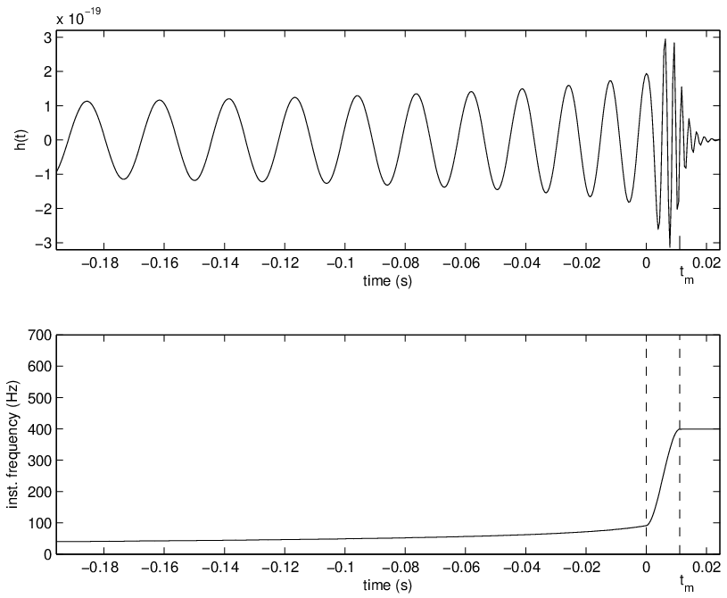
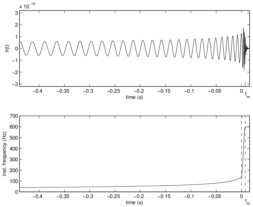
(a) (b)
4 Results
To use the BP test we first need the distribution of under . There is no analytic expression for the distribution of the BP statistic so we have used a Monte Carlo simulation to estimate them. As our test signals have different lengths we generated three null distributions, one for each . In each case we generated instances of simulated LIGO noise and calculated for each of them with chirplet path lengths drawn from the set . These random trials give an approximation to the distributions of under for each . Using our empirical distributions we can estimate the -value for an observed .
To test detection efficiency, we first constructed normalised test signals using the model described in Section 3.2. For each and we generated instances of noise and injected the signal at that level. The BP statistic was calculated, as was , and we determined the detection probability for a given by counting the number of . Figure 3 gives the detection probabilities as a function of (the Receiver Operating Characteristic curve) for , and . For comparison, we also give an ROC curve obtained using matched filtering to detect the signal. For these curves has been chosen to give a good match to the ROC curve obtained via the BP test. From this it can be seen that the BP statistic is about half as sensitive as matched filtering. Since the distance to the source is inversely proportional to the overall signal amplitude, we can consider the BP test to have a seeing distance about half that of matched filtering.
(a)


(b)


(c)


In Figure 3 we also give the detection probability as a function of (or equivalently, inverse distance to the source) for = , and . The corresponding distances at are for , for and for . This shows that, for example, at a false alarm probability of we can see an event out to with a false dismissal probability of about . Note that since we have averaged the signal amplitude over sky positions and orientations, an optimally aligned and positioned source could be detected much farther away.
In the above comparison we are injecting a known signal into noise and using the same (normalised) signal as our template for matched filtering. Real signals in interferometer data will have unknown parameters, and a bank of templates using discrete values of the parameters (mass, spin etc) is needed to cover the range of physically plausible coalescences. Since a real signal has parameters drawn from a continuum there will usually be some degree of mismatch between the signal and templates in the bank. As such, the comparison above is very conservative in comparing the BP test with the most favourable matched filter detection scenario, one which is unlikely to be attained in practise. A more realistic benchmark is obtained by examining the performance of the BP test when the signal parameters are chosen at random from a range of values. Here we present a comparison of the BP test with detection via a bank of templates, and with another method employed in searches for unmodelled signals, the excess power statistic [13].
We first created a bank of templates using discrete values for the parameters. Although our complete signal model contains a large number of free parameters, for simplicity we chose to only vary , and , as these have the greatest effect on the waveform. For the same reason we have used equal spacing in all parameters, rather than attempting to construct a template bank spaced to give equal overlap between adjacent templates. While methods exist to construct optimally-spaced template banks, our templates have the additional complication of including merger and ringdown components.
For each of the signal lengths , and we generated a bank of normalised templates using the criteria that
- 1.
The range of masses and is chosen so that the length of the signals range from to samples.
- 2.
The spin ranges from to .
- 3.
The spacing between masses and spins is chosen so that the minimal match of a signal with parameters drawn from the range of parameters is at least .
For each we then generated test signals with mass and spin parameters drawn at random from the appropriate range, and injected them into simulated LIGO noise with . The resulting data was used to calculate a BP statistic for each segment. Comparing the BP statistics with the empirical null distribution as above, we obtained the ROC curves shown in Figure 4. Searching for the same signals via matched filtering, we found that the ROC curves matched well when the signals were injected with around – in other words, the BP test sees about as far as the template bank.


(a) (b)

(c)
We performed a similar analysis using the excess power statistic, which is optimal when the only known features of the signal are the duration and bandwidth [13]. The excess power statistic is simply the power calculated using (4) where the integration is performed over the bandwitch of the expected signals, taken to be – Hz in this instance. Under this has a distribution with degrees of freedom twice the number of frequency bins. Using the excess power statistic, we found that the ROC curves matched those of the BP test in Figure 4 well when was around .
5 Conclusion
Chirplet path pursuit has previously been shown to be effective at detecting a broad class of chirp-like but otherwise unmodelled signals in coloured noise [19]. In this paper we have demonstrated that the method can be successfully applied to the problem of detecting test signals with similar characteristics to those expected from binary black hole coalescence. The method is able to detect a range of signals of modest strength hidden in simulated LIGO noise, and exhibits somewhat better statistical power than the excess power test.
As with other methods for detecting bursts, in real LIGO noise there is the difficulty of distinguishing genuine gravitational wave signals from instrumental and environmental events. For matched filter searches the discriminator can be used to reject signals that do not have the correct distribution of power across frequency bands, however this requires that the gravitational waveform be known [28]. This discriminator is not applicable to chirplet path pursuit since the signal is not known and we do not impose any assumptions on the distribution of power. Instead we would rely on the methods being employed in current searches: requiring events to be coincident across multiple detectors, vetoing events based on environmental channels, and testing if waveforms measured in different detectors are consistent [29, 18].
As expected for a non-parametric method, chirplet path pursuit is not as sensitive as matched filtering using a template bank, nevertheless our comparison shows that the method has similar effectiveness to matched filtering for a signal that is roughly times as strong. Significantly, since the method is sensitive to a wide range of chirp-like signals, an exact model of the signals to be detected is not necessary. This makes the method particularly of interest in situations where the signal is unmodelled or poorly modelled, as is the case for the late inspiral and merger components of intermediate mass black hole coalescences.
References
References
- [1]
http://www.ligo.caltech.edu - [2] Damour T, Iyer B R and Sathyaprakash B S 2001 Phys. Rev. D 60 044023
- [3] Apostolatos T A, Cutler C, Sussman G J and Thorne K S 1994 Phys. Rev. D 49 6274
- [4] Sathyaprakash B S and Schutz B F 2003 Class. Quantum Grav. 20 S209–S218
- [5] Gair J R, Barack L, Creighton T, Cutler C, Larson S L, Phinney E S and Vallisneri M 2004 Class. Quantum Grav. 21 S1595–S1606
- [6] Buonanno A, Chen Y and Vallisneri M 2003 Phys. Rev. D 67 024016
- [7] Pan Y, Buonanno A, Chen Y and Vallisneri M 2004 Phys. Rev. D 69 104017
- [8] Buonanno A, Chen Y, Pan Y, Tagoshi H, and Vallisneri M 2005 Phys. Rev. D 72 084027
- [9] Goggin L 2006 Class. Quantum Grav. 23 S709–S713
- [10] Pretorius F 2005 Phys. Rev. Lett. 95 121101
- [11] Baker J G, Centrella J, Choi D I, Koppitz M and van Meter J 2006 Phys. Rev. D 73 104002
- [12] Anderson W G and Balasubramanian R 1999 Phys. Rev. D 60 102001
- [13] Anderson W G, Brady P R, Creighton J D E and Flanagan É É 2001 Phys. Rev. D 63 142003
- [14] Sylvestre J 2002 Phys. Rev. D 66 102004
- [15] Klimenko S and Mitselmakher G 2004 Class. Quantum Grav. 21 S1819–S1830
- [16] Chatterji S 2005 The search for gravitational wave bursts in data from the second LIGO science run Ph.D. thesis Massachusetts Institute of Technology
- [17] Chassande-Mottin É and Pai A 2006 Phys. Rev. D 73 042003
- [18] A Abbott et al 2007 Class. Quantum Grav. 24 5343–5369
- [19] Candès E J, Charlton P R and Helgason H 2008 Appl. Comput. Harmon. Anal. 24 14–40
- [20] Jenet F A and Prince T A 2000 Phys. Rev. D 62 122001
- [21] Joksch H C 1966 J. Math. Anal. Appl. 14 191–197
- [22] Benjamini Y and Hochberg Y 1995 J. R. Statist. Soc. B 57 289–300
- [23] Grishchuk L P, Lipunov V M, Postnov K A, Prokhorov M E and Sathyaprakash B S 2001 Physics-Uspekhi 44 1–51
- [24] Flanagan É É and Hughes S 1998 Phys. Rev. D 57 4535
- [25] The LIGO Scientific Collaboration LAL Software Documentation http://www.lsc-group.phys.uwm.edu/lal/slug/nightly/doc/lsd-nightly.pdf
- [26] Thorne K S 1987 300 Years of Gravitation ed Hawking S W and Israel W (Cambridge University Press)
- [27] P Ajith et al 2007 Class. Quantum Grav. 24 S689–S699
- [28] Allen B 2005 Phys. Rev. D 71 062001
- [29] A Abbott et al 2005 Phys. Rev. D 72 122004
- [30] Candès E J 2002 Multiscale chirplets and near-optimal recovery of chirps Tech. rep. Stanford University
Appendix
In this appendix we present the scheme used for calculating chirplet coefficients of discretised data. The data is discretely sampled at intervals of duration . Notionally, this discretises the time-frequency plane into points where and . Points in the time-frequency plane are considered to be vertices in a directed graph where the weight of the arc connecting two vertices is given by the local correlation of with the corresponding chirplet.
Consider chirplets supported on the interval . At scale , this interval has length samples. While there are many ways to discretise chirplets on this interval, it is convenient to choose the spacing of the frequency parameter to correspond with the bins of a discrete Fourier transform, and choose the spacing of the chirp parameter so that at the end of the interval the instantaneous frequency has changed by a whole number of bins. Thus our dictionary of chirplets is indexed by scale index , frequency index and chirp index , and the (unnormalised) discrete chirplet is given by
| (17) |
where the phase is
| (18) |
The discretised instantaneous frequency is
| (19) |
Such a chirplet has initial frequency and rises to frequency at a rate of . Since we only deal with real signals, the range of the chirp index is chosen to restrict the chirplets to non-negative frequencies up to Nyquist, thus .
In general, the inner product (4) for a noise process with covariance matrix is , where is the conjugate transpose of . For our noise model the Fourier matrices diagonalise , and so where and are the eigenvalues of . Calculating for a chirplet supported on a dyadic interval is equivalent to calculating the inner product of with a chirplet supported on . As the time index of the first sample in is , let be the samples of restricted to . Then to find we pad and to length with zeroes and FFT. In discrete form, the inner product then reduces to
| (20) |
where . If has indices , then after normalising, is the weight of the arc connecting to .
To calculate the BP statistic we must find the total weight of connected, non-overlapping chirplet paths in the time-frequency plane starting at and ending at . To keep the number of arcs manageable we further restrict our chirplet paths to those supported on a recursive dyadic partition (RDP) of constructed using the following definition [30]:
- 1.
The trivial partition is an RDP.
- 2.
If is an RDP, then so is the partition obtained by splitting any interval into two adjacent dyadic intervals.
This means that, for example, that is a recursive dyadic partition of , but is not. The total weight of a chirplet path supported on is then
| (21) |