跳到论文正文
W Papers独立论文阅读器 arXiv:0806.4415 论文正文 计算阅读时间 · 0%
引用这篇论文根据当前论文元数据生成,正式投稿前建议核对。


License: arXiv.org perpetual non-exclusive license
arXiv:0806.4415v2 [cs.IT] 06 Jan 2009

On 3-receiver broadcast channels with 2-degraded message sets

Chandra Nair Affiliation: Department of Information Engineering
Chinese University of Hong Kong
Sha Tin, N.T., Hong Kong
Email: chandra@ie.cuhk.edu.hk
   Zizhou Vincent Wang Affiliation: Department of Information Engineering
Chinese University of Hong Kong
Sha Tin, N.T., Hong Kong
Email: zzwang6@ie.cuhk.edu.hk
Abstract

We consider a broadcast channel with 3 receivers and 2 messages (M0,M1)(M_{0},M_{1}) where two of the three receivers need to decode messages (M0,M1)(M_{0},M_{1}) while the remaining one just needs to decode the message M0M_{0}. We study the best known inner and outer bounds under this setting, in an attempt to find the deficiencies with the current techniques of establishing the bounds. We produce a simple example where we are able to explicitly evaluate the inner bound and show that it differs from the general outer bound. For a class of channels where the general inner and outer bounds differ, we use a new argument to show that the inner bound is tight.

I Introduction

The broadcast channel with degraded message sets was initially studied by Kórner and Märton [1] for two receivers and more recently in [2, 3, 4] for three and more receivers. Kórner and Märton [1] established the capacity region for the degraded message sets with two receivers and some capacity regions for three or more receivers were established [2, 3] by showing that the straightforward extension of the inner bound in [1] was optimal. In [4], an idea called indirect decoding was introduced and the authors showed that this could be used to enhance (in some cases strictly) the straightforward extension of the inner bound by Kórner and Märton. Unfortunately, the new inner bounds [4] become quite messy and unwieldy due to the introduction of many auxiliary random variables. However there is still one class of broadcast channels with degraded message sets where the idea of indirect decoding does not yield any region better than the straightforward extension of the Kórner and Märton inner bound, and this is the scenario of interest here.

Consider a 3-receiver broadcast channel with 2 messages (M0,M1)(M_{0},M_{1}) with the following decoding requirement. Receivers Y1Y_{1} and Y2Y_{2} need to decode both messages (M0,M1)(M_{0},M_{1}) while receiver Y3Y_{3} needs to decode only message M0M_{0}. The traditional inner and outer bounds presented below remain the best known inner and outer bounds for this class of broadcast channels. In this paper we look at the general inner and outer bounds for this scenario in a greater detail. We show that these bounds differ in general, and that there is a class of channels where the inner bound is tight and the outer bound is weak.

There are two main contributions in this paper: the first one is the technique (same spirit as Mrs. Gerber’s lemma [5]) used to evaluate the boundary of a particular inner bound; the second is the use of a (12+ϵ\frac{1}{2}+\epsilon)-codebook11 1 An η\eta-codebook is used to denote a codebook whose probability of error is bounded above by η\eta. rather than an ϵ\epsilon-codebook to establish the capacity region.

Bound 1

The union of the following set of rate pairs (R0,R1)(R_{0},R_{1}) satisfying

R0\displaystyle R_{0} ≤I⁡(U,Y3)\displaystyle\leq I(U;Y_{3})
R1\displaystyle R_{1} ≤min⁡{I⁡(X;Y1|U),I⁡(X;Y2|U)}\displaystyle\leq\min\{I(X;Y_{1}|U),I(X;Y_{2}|U)\}
R0+R1\displaystyle R_{0}+R_{1} ≤min⁡{I⁡(X,Y1),I⁡(X,Y2)}\displaystyle\leq\min\{I(X;Y_{1}),I(X;Y_{2})\}

over all pairs of random variables (U,X)(U,X) such that U→X→(Y1,Y2,Y3)U\to X\to(Y_{1},Y_{2},Y_{3}) forms a Markov chain constitutes an inner bound to the capacity region.

Bound 2

The union over the set of rate pairs (R0,R1)(R_{0},R_{1}) satisfying

R0\displaystyle R_{0} ≤min⁡{I⁡(U1,Y3),I⁡(U2,Y3)}\displaystyle\leq\min\{I(U_{1};Y_{3}),I(U_{2};Y_{3})\}
R0+R1\displaystyle R_{0}+R_{1} ≤min{I(U1;Y3)+I(X;Y1|U1),\displaystyle\leq\min\{I(U_{1};Y_{3})+I(X;Y_{1}|U_{1}),
I(U2;Y3)+I(X;Y2|U2)}\displaystyle\qquad I(U_{2};Y_{3})+I(X;Y_{2}|U_{2})\}
R0+R1\displaystyle R_{0}+R_{1} ≤min⁡{I⁡(X,Y1),I⁡(X,Y2)}\displaystyle\leq\min\{I(X;Y_{1}),I(X;Y_{2})\}

over all possible choices of random variables (U1,U2,X)(U_{1},U_{2},X) such that (U1,U2)→X→(Y1,Y2,Y3)(U_{1},U_{2})\to X\to(Y_{1},Y_{2},Y_{3}) forms a Markov chain constitutes an outer bound for this channel.

The above bounds are traditional, i.e. can be obtained using standard techniques. The inner bound is a straightforward extension of the achievability argument in [1] and the outer bound can be deduced by arguments in [6, 7], etc.

Remark 1

It is also possible to include the constraint

R0≤min⁡{I⁡(U1,Y1),I⁡(U2,Y2)}R_{0}\leq\min\{I(U_{1};Y_{1}),I(U_{2};Y_{2})\}

into the outer bound. However, it is quite straightforward to show that the region obtained by adding this inequality is identical to the bound we presented.

These bounds are known to be tight in all of the following special cases,

  • •

    Receiver Y1Y_{1} is a less noisy receiver than Y3Y_{3} and Y2Y_{2} is a less noisy receiver than Y3Y_{3} [2, 4],

  • •

    Y3Y_{3} is a deterministic function of XX,

  • •

    Y1Y_{1} is a more capable receiver than Y2Y_{2} (or vice-versa),

  • •

    Y3Y_{3} is a more capable receiver than Y2Y_{2} (or Y1Y_{1}),

The last two cases are very straightforward and the proof is omitted. When Y3Y_{3} is a deterministic function of XX, note that it is not difficult to show that by taking the convex closure of the regions obtained by setting (i)(i) U=Y3U=Y_{3} and (i​i)(ii) U=∅U=\emptyset in the inner bound exhausts the following region,

R0\displaystyle R_{0} ≤H⁡(Y3)\displaystyle\leq H(Y_{3})
R0+R1\displaystyle R_{0}+R_{1} ≤min⁡{I⁡(X,Y1),I⁡(X,Y2)}\displaystyle\leq\min\{I(X;Y_{1}),I(X;Y_{2})\}

and this clearly forms an outer bound to the capacity region.

One class of channels that does not fall into any of the cases is the following channel shown in Figure 1 below. The channel X→(Y1,Y2)X\to(Y_{1},Y_{2}) represents a binary skew-symmetric (BSSC) broadcast channel [7, 8] and the channel X→Y3X\to Y_{3} represents a binary symmetric (BSC) with crossover probability pp, with 0≤p≤120\leq p\leq\frac{1}{2}.

Refer to caption
Fig. 1: 3-receiver broadcast channel

In the next section we evaluate Bound 1 for this channel. Based on the symmetry, it is very natural to believe that the auxiliary channel U→XU\to X must be a BSC with some cross over probability ss. In the next section, we prove that this is indeed the case. This uses a technique similar in spirit to Wyner and Ziv’s technique of using Mrs. Gerber’s lemma [5]. We will also show that the Bound 2 yields a strictly larger region for this channel. Finally, we will show that the region represented by Bound 1 constitutes the capacity region for this channel.

II Evaluation of the inner bound

In the evaluation of the inner bound, we divide the range 0≤p≤120\leq p\leq\frac{1}{2} into two regions, 0≤p≤pm​a​x0\leq p\leq p_{max} and pm​a​x≤p≤12p_{max}\leq p\leq\frac{1}{2}, where pm​a​x∈[0,12]p_{max}\in[0,\frac{1}{2}] is the unique solution of

1−h⁡(p)=h⁡(14)−12;1-h(p)=h(\frac{1}{4})-\frac{1}{2};

i.e. the value of pp at which capacity of the BSC matches the term maxp⁡(x)⁡min⁡{I⁡(X,Y1),I⁡(X,Y2)}\max_{p(x)}\min\{I(X;Y_{1}),I(X;Y_{2})\}. The numerical value of pm​a​x≈0.184p_{max}\approx 0.184.

II-A Evaluation of the inner bound, 0≤p≤pm​a​x0\leq p\leq p_{max}

In the region 0≤p≤pm​a​x0\leq p\leq p_{max} it is straightforward to see that the inner bound reduces to the following region (obtained via a time-division between the two auxiliary channels: (i)(i) U=∅U=\emptyset and (i​i)(ii) U=XU=X, and in each case, setting P⁡(X=0)=0.5{\rm P}(X=0)=0.5),

R0+R1≤h⁡(14)−12,R_{0}+R_{1}\leq h(\frac{1}{4})-\frac{1}{2},

which clearly matches the outer bound (Bound 2). Thus for 0≤p≤pm​a​x≈0.1840\leq p\leq p_{max}\approx 0.184, the inner and outer bounds are tight and give the capacity region.

II-B Evaluation of the inner bound, pm​a​x≤p≤12p_{max}\leq p\leq\frac{1}{2}

Let 𝒰={1,2,…,m}{\cal U}=\{1,2,...,m\} and let P⁡(U=i)=ui{\rm P}(U=i)=u_{i} and P⁡(X=0|U=i)=si{\rm P}(X=0|U=i)=s_{i}. Further, let

h⁡(x)=−x​log2​x−(1−x)​log2⁡(1−x)h(x)=-x\log_{2}x-(1-x)\log_{2}(1-x)

denote the binary entropy function.

Using these notations we have,

I⁡(U,Y3)\displaystyle I(U;Y_{3}) =h⁡(∑iui​(si​(1−p)+(1−si)​p))\displaystyle=h(\sum_{i}u_{i}(s_{i}(1-p)+(1-s_{i})p))
−∑iuih(si(1−p)+(1−si)p)\displaystyle\qquad-\sum_{i}u_{i}h(s_{i}(1-p)+(1-s_{i})p)
I⁡(X;Y1|U)\displaystyle I(X;Y_{1}|U) =∑iui​h​(si2)−∑iui​si\displaystyle=\sum_{i}u_{i}h(\frac{s_{i}}{2})-\sum_{i}u_{i}s_{i}
I⁡(X;Y2|U)\displaystyle I(X;Y_{2}|U) =∑iui​h​(1−si2)−∑iui​(1−si)\displaystyle=\sum_{i}u_{i}h(\frac{1-s_{i}}{2})-\sum_{i}u_{i}(1-s_{i})
I⁡(X,Y1)\displaystyle I(X;Y_{1}) =h⁡(∑iui​si2)−∑iui​si\displaystyle=h(\sum_{i}\frac{u_{i}s_{i}}{2})-\sum_{i}u_{i}s_{i}
I⁡(X,Y2)\displaystyle I(X;Y_{2}) =h⁡(∑iui​(1−si)2)−∑iui​(1−si).\displaystyle=h(\sum_{i}\frac{u_{i}(1-s_{i})}{2})-\sum_{i}u_{i}(1-s_{i}).

Define 𝒰~={1,2,…,m}×{1,2}\tilde{{\cal U}}=\{1,2,...,m\}\times\{1,2\}, P⁡(U~=(i,1))=ui2{\rm P}(\tilde{U}=(i,1))=\frac{u_{i}}{2}, P⁡(X=0|U~=(i,1))=si{\rm P}(X=0|\tilde{U}=(i,1))=s_{i}, P⁡(U~=(i,2))=ui2{\rm P}(\tilde{U}=(i,2))=\frac{u_{i}}{2}, and P⁡(X=0|U~=(i,2))=1−si{\rm P}(X=0|\tilde{U}=(i,2))=1-s_{i}. This induces an X~\tilde{X} with P⁡(X~=0)=12P(\tilde{X}=0)=\frac{1}{2}. It is straightforward to see the following:

I⁡(U~,Y~3)\displaystyle I(\tilde{U};\tilde{Y}_{3}) ≥I⁡(U,Y3)\displaystyle\geq I(U;Y_{3})
I⁡(X~;Y~1|U~)\displaystyle I(\tilde{X};\tilde{Y}_{1}|\tilde{U}) =I⁡(X~;Y~2|U~)=12​(I⁡(X;Y1|U)+I⁡(X;Y2|U))\displaystyle=I(\tilde{X};\tilde{Y}_{2}|\tilde{U})=\frac{1}{2}(I(X;Y_{1}|U)+I(X;Y_{2}|U))
≥min⁡{I⁡(X;Y1|U),I⁡(X;Y2|U)}\displaystyle\geq\min\{I(X;Y_{1}|U),I(X;Y_{2}|U)\}
I⁡(X~,Y~1)\displaystyle I(\tilde{X};\tilde{Y}_{1}) =I⁡(X~,Y~2)≥12​(I⁡(X,Y1)+I⁡(X,Y2))\displaystyle=I(\tilde{X};\tilde{Y}_{2})\geq\frac{1}{2}(I(X;Y_{1})+I(X;Y_{2}))

From this it follows that for every UU replacing UU by U~\tilde{U} leads to a larger achievable region. Hence to evaluate Bound 1, it suffices to maximize over all auxiliary random variables of the form UU defined by: 𝒰={1,2,…,m}×{1,2}{\cal U}=\{1,2,...,m\}\times\{1,2\}, P⁡(U=(i,1))=ui2{\rm P}(U=(i,1))=\frac{u_{i}}{2}, P⁡(X=0|U=(i,1))=si{\rm P}(X=0|U=(i,1))=s_{i}, P⁡(U=(i,2))=ui2{\rm P}(U=(i,2))=\frac{u_{i}}{2}, and P⁡(X=0|U=(i,2))=1−si{\rm P}(X=0|U=(i,2))=1-s_{i}.

Under this notation we have the following expression for the rate region given in Bound 1,

R0\displaystyle R_{0} ≤I⁡(U,Y3)\displaystyle\leq I(U;Y_{3})
=h⁡(12)−∑iui​h​(si​(1−p)+(1−si)​p),\displaystyle=h\big(\frac{1}{2}\big)-\sum_{i}u_{i}h(s_{i}(1-p)+(1-s_{i})p),
R1\displaystyle R_{1} ≤min⁡{I⁡(X;Y1|U),I⁡(X;Y2|U)}\displaystyle\leq\min\{I(X;Y_{1}|U),I(X;Y_{2}|U)\}
=∑iui2​(h⁡(si2)+h⁡(1−si2))−12,\displaystyle=\sum_{i}\frac{u_{i}}{2}\left(h(\frac{s_{i}}{2})+h(\frac{1-s_{i}}{2})\right)-\frac{1}{2},
R0+R1\displaystyle R_{0}+R_{1} ≤min⁡{I⁡(X,Y1),I⁡(X,Y2)}\displaystyle\leq\min\{I(X;Y_{1}),I(X;Y_{2})\}
=h⁡(14)−12.\displaystyle=h\big(\frac{1}{4}\big)-\frac{1}{2}.

Using the symmetry of the function h⁡(x)=h⁡(1−x)h(x)=h(1-x) we note that

h⁡(si​(1−p)+(1−si)​p)=h⁡((1−si)​(1−p)+si​p)h(s_{i}(1-p)+(1-s_{i})p)=h((1-s_{i})(1-p)+s_{i}p)

and thus the above region is constant under the transformation si→1−sis_{i}\to 1-s_{i}, implying we can restrict sis_{i} to take values only in 0≤si≤120\leq s_{i}\leq\frac{1}{2}.

Before we proceed to determine the boundary of this region, we prove the following lemma.

II-C An inequality for a class of functions

Lemma 1

Let f⁡(x)f(x) and g⁡(x)g(x) be two non-negative and strictly increasing functions that are differentiable in the region x∈[x1,x2]x\in[x_{1},x_{2}]. Further assume that f(1)​(x)g(1)​(x)\frac{f^{(1)}(x)}{g^{(1)}(x)} is a decreasing function, where f(1)​(x)f^{(1)}(x) and g(1)​(x)g^{(1)}(x) denote the derivatives of the function. Given any u,0≤u≤1u,0\leq u\leq 1, let xi​n​tx_{int} be uniquely defined according to f⁡(xi​n​t)=u​f​(x1)+(1−u)​f​(x2).f(x_{int})=uf(x_{1})+(1-u)f(x_{2}). Then the following holds,

g⁡(xi​n​t)≤u​g​(x1)+(1−u)​g​(x2).g(x_{int})\leq ug(x_{1})+(1-u)g(x_{2}).
Proof:

We have u⁡(f⁡(xi​n​t)−f⁡(x1))=(1−u)​(f⁡(x2)−f⁡(xi​n​t))u(f(x_{int})-f(x_{1}))=(1-u)(f(x_{2})-f(x_{int})), and we wish to show that u⁡(g⁡(xi​n​t)−g⁡(x1))≤(1−u)​(g⁡(x2)−g⁡(xi​n​t))u(g(x_{int})-g(x_{1}))\leq(1-u)(g(x_{2})-g(x_{int})). Since all the terms are positive, this reduces to showing f(x int ) - f(x 1 ) g(x int ) - g(x 1 ) ≥ f(x 2 ) - f(x int ) g(x 2 ) - g(x int ) . However, this is immediate as shown below.

From the fact that f(1)​(x)g(1)​(x)\frac{f^{(1)}(x)}{g^{(1)}(x)} is a decreasing function, we have ∫ x 1 x int f (1) (x) dx ∫ x 1 x int g (1) (x) dx ≥ f (1) (x int ) g (1) (x int ) ≥ ∫ x int x 2 f (1) (x) dx ∫ x int x 2 g (1) (x) dx ∎

Repeated applications of Lemma 1 leads to the following corollary - potentially of independent interest.

Corollary 1

Let f⁡(x)f(x) and g⁡(x)g(x) be two non-negative and strictly increasing functions that are differentiable in the region x∈[x1,x2]x\in[x_{1},x_{2}]. Further assume that f(1)​(x)g(1)​(x)\frac{f^{(1)}(x)}{g^{(1)}(x)} is a decreasing function, where as before f(1)​(x)f^{(1)}(x) and g(1)​(x)g^{(1)}(x) denote the derivatives of the function. Given any ui≥0,∑iui=1u_{i}\geq 0,\sum_{i}u_{i}=1, and yi∈[x1,x2]y_{i}\in[x_{1},x_{2}], let xi​n​tx_{int} be uniquely defined according to f⁡(xi​n​t)=∑iui​f​(yi).f(x_{int})=\sum_{i}u_{i}f(y_{i}). Then the following holds

g⁡(xi​n​t)≤∑iui​g​(yi).g(x_{int})\leq\sum_{i}u_{i}g(y_{i}).

II-D Determining the boundary rate pairs

We use the Corollary 1 to determine the boundary of the region. We make the following identifications, let f⁡(x)=h⁡(x2)+h⁡(1−x2)−1f(x)=h(\frac{x}{2})+h(\frac{1-x}{2})-1, and g⁡(x)=h⁡(x⁡(1−p)+(1−x)​p)g(x)=h(x(1-p)+(1-x)p). Observe that f⁡(x)f(x) and g⁡(x)g(x) are increasing differentiable functions in the region [0,12][0,\frac{1}{2}].

Claim 1

For 16≤p≤12\frac{1}{6}\leq p\leq\frac{1}{2}, the ratio of the derivatives f(1)​(x)g(1)​(x)\frac{f^{(1)}(x)}{g^{(1)}(x)} is a decreasing function.

The proof of this fact is found in the Appendix.

(Numerical simulations indicate that this is true for pm​i​n≤p≤12p_{min}\leq p\leq\frac{1}{2} for pm​i​n≈0.05p_{min}\approx 0.05, but for the purposes of establishing the inner bound clearly this region of pp suffices, as 16≤pm​a​x≈0.184\frac{1}{6}\leq p_{max}\approx 0.184).

Remark 2

By combining Claim 1 and Corollary 1 note that h​(p∗f−1​(y))h(p*f^{-1}(y)) is convex in yy, and this is very similar to Mrs. Gerber’s Lemma [5].

Now let si​n​ts_{int} be defined according to

h⁡(si​n​t2)+h⁡(1−si​n​t2)=∑iui​(h⁡(si2)+h⁡(1−si2)).h(\frac{s_{int}}{2})+h(\frac{1-s_{int}}{2})=\sum_{i}u_{i}\left(h\big(\frac{s_{i}}{2}\big)+h\big(\frac{1-s_{i}}{2}\big)\right).

Then from Corollary 1, for pm​i​n≤p≤12p_{min}\leq p\leq\frac{1}{2} we have

h⁡(12)−∑iui​h​(si​(1−p)+(1−si)​p)\displaystyle h\big(\frac{1}{2}\big)-\sum_{i}u_{i}h(s_{i}(1-p)+(1-s_{i})p)
≤h⁡(12)−h⁡(si​n​t​(1−p)+(1−si​n​t)​p).\displaystyle\quad\leq h\big(\frac{1}{2}\big)-h(s_{int}(1-p)+(1-s_{int})p).

This implies that the optimal auxiliary channel U→XU\to X is a BSC with a cross-over probability ss and P⁡(U=0)=12{\rm P}(U=0)=\frac{1}{2}. Thus for pm​a​x≤p≤12p_{max}\leq p\leq\frac{1}{2}, the boundary is characterized by the pair of points of the form,

R0\displaystyle R_{0} =1−h⁡(s⁡(1−p)+(1−s)​p),\displaystyle=1-h(s(1-p)+(1-s)p),
R1\displaystyle R_{1} =min{12(h(s2)+h(1−s2)−1),\displaystyle=\min\left\{\frac{1}{2}\left(h\big(\frac{s}{2}\big)+h\big(\frac{1-s}{2}\big)-1\right)\right., (1)
h(14)−32+h(s(1−p)+(1−s)p)},\displaystyle\quad\left.h\big(\frac{1}{4}\big)-\frac{3}{2}+h(s(1-p)+(1-s)p)\right\},

for 0≤s≤120\leq s\leq\frac{1}{2}. The second term in R1R_{1} comes from taking into account the sum rate constraint,

R0+R1≤h⁡(14)−12.R_{0}+R_{1}\leq h\big(\frac{1}{4}\big)-\frac{1}{2}.

A simple calculation shows that for po≤p≤12p_{o}\leq p\leq\frac{1}{2} one can ignore the sum rate constraint, where po=3−12​3≈0.211p_{o}=\frac{\sqrt{3}-1}{2\sqrt{3}}\approx 0.211. This pop_{o} corresponds to the smallest value of pp where the convex region characterized by the pairs

R0\displaystyle R_{0} =1−h⁡(s⁡(1−p)+(1−s)​p),\displaystyle=1-h(s(1-p)+(1-s)p),
R1\displaystyle R_{1} =12​(h⁡(s2)+h⁡(1−s2)−1).\displaystyle=\frac{1}{2}\left(h\big(\frac{s}{2}\big)+h\big(\frac{1-s}{2}\big)-1\right).

has a slope of −1-1 at the point (R0,R1)=(0,h⁡(14)−12)(R_{0},R_{1})=\left(0,h\big(\frac{1}{4}\big)-\frac{1}{2}\right).

Therefore the inner bound has three different expressions:

  • •

    0≤p≤pm​a​x0\leq p\leq p_{max}: the inner bound reduces to R0+R1≤h⁡(14)−12R_{0}+R_{1}\leq h\big(\frac{1}{4}\big)-\frac{1}{2},

  • •

    pm​a​x≤p≤pop_{max}\leq p\leq p_{o}: the inner bound is given by equation (1) where all inequalities are necessary,

  • •

    po≤p≤12p_{o}\leq p\leq\frac{1}{2}: the inner bound is characterized by pair of points of the form

    R0\displaystyle R_{0} =1−h⁡(s⁡(1−p)+(1−s)​p),\displaystyle=1-h(s(1-p)+(1-s)p),
    R1\displaystyle R_{1} =12​(h⁡(s2)+h⁡(1−s2)−1).\displaystyle=\frac{1}{2}\left(h\big(\frac{s}{2}\big)+h\big(\frac{1-s}{2}\big)-1\right).

II-E Comparison with the outer bound

To show that the outer bound gives a larger region, we produce a particular choice of the pair (U1,U2,X)(U_{1},U_{2},X). Consider a U1,U2U_{1},U_{2} defined as follows,

P⁡(U1=1)=P⁡(U2=1)=u,\displaystyle{\rm P}(U_{1}=1)={\rm P}(U_{2}=1)=u,
P⁡(U1=2)=P⁡(U2=2)=1−u,\displaystyle{\rm P}(U_{1}=2)={\rm P}(U_{2}=2)=1-u,
P⁡(X=0|U1=1)=P⁡(X=1|U2=1)=1,\displaystyle{\rm P}(X=0|U_{1}=1)={\rm P}(X=1|U_{2}=1)=1,
P⁡(X=0|U1=2)=P⁡(X=1|U2=2)=s,\displaystyle{\rm P}(X=0|U_{1}=2)={\rm P}(X=1|U_{2}=2)=s,

where s=0.5−u1−us=\frac{0.5-u}{1-u} for 0≤u≤0.50\leq u\leq 0.5. Existence of the triple (U1,U2,X)(U_{1},U_{2},X) is guaranteed by the consistent distribution on XX. Substituting this choice into Bound 2 we obtain Region A given by,

R0\displaystyle R_{0} ≤1−(1−u)​h​(s⁡(1−p)+(1−s)​p)−u​h​(p),\displaystyle\leq 1-(1-u)h\big(s(1-p)+(1-s)p\big)-uh\big(p\big),
R1\displaystyle R_{1} ≤(1−u)​h​(s2)−12+u,\displaystyle\leq(1-u)h\big(\frac{s}{2}\big)-\frac{1}{2}+u,
R0+R1\displaystyle R_{0}+R_{1} ≤h⁡(14)−12.\displaystyle\leq h\big(\frac{1}{4}\big)-\frac{1}{2}.

Figure 2 plots Region A and Bound 1 for p=14p=\frac{1}{4}. Observe that Region AA is larger than Bound 1, and hence the Bounds 1 and 2 do not match for the 3-receiver channel shown in Figure 1. This implies the following corollary.

Refer to caption
Fig. 2: Comparing Bound 1 and Region A for p=14p=\frac{1}{4}
Corollary 2

There exists a class of channels, given in Figure 1, for which the inner and outer bounds (i.e. Bounds 1 and 2) do not match.

III Revisiting outer bound

We now show that the inner bound is tight for the channel shown in Figure 1.

Let π:{0,1}↦{0,1};π⁡(0)=1,π⁡(1)=0\pi:\{0,1\}\mapsto\{0,1\};\pi(0)=1,\pi(1)=0.

Consider an ϵ\epsilon-codebook {xm0,m1n,1≤m0≤2n​R0,1≤m1≤2n​R1,𝒜m0,m1⊆𝒴1n,ℬm0,m1⊆𝒴2n,𝒞m0⊆𝒴3n\{x^{n}_{m_{0},m_{1}},1\leq m_{0}\leq 2^{nR_{0}},1\leq m_{1}\leq 2^{nR_{1}},{\cal A}_{m_{0},m_{1}}\subseteq{\cal Y}_{1}^{n},{\cal B}_{m_{0},m_{1}}\subseteq{\cal Y}_{2}^{n},{\cal C}_{m_{0}}\subseteq{\cal Y}_{3}^{n}}, where the disjoint sets 𝒜m0,m1,ℬm0,m1,𝒞m0{\cal A}_{m_{0},m_{1}},{\cal B}_{m_{0},m_{1}},{\cal C}_{m_{0}} represent the decoding maps. From the skew symmetry of the channels X→(Y1,Y2)X\to(Y_{1},Y_{2}) and the symmetry in channel X→Y3X\to Y_{3}, it is clear that {π(xm0,m1n),1≤m0≤2n​R0,1≤m1≤2n​R1,π(ℬm0,m1)⊆𝒴1n,π(𝒜m0,m1)⊆𝒴2n,π(𝒞m0)⊆𝒴3n\{\pi(x^{n}_{m_{0},m_{1}}),1\leq m_{0}\leq 2^{nR_{0}},1\leq m_{1}\leq 2^{nR_{1}},\pi({\cal B}_{m_{0},m_{1}})\subseteq{\cal Y}_{1}^{n},\pi({\cal A}_{m_{0},m_{1}})\subseteq{\cal Y}_{2}^{n},\pi({\cal C}_{m_{0}})\subseteq{\cal Y}_{3}^{n}} represents a valid ϵ\epsilon-codebook as well.

From these two codes, construct a new codebook (with error bounded by 12+ϵ\frac{1}{2}+\epsilon) and size 2n​R0×2n​R1+12^{nR_{0}}\times 2^{nR_{1}+1} as follows: The codewords are indexed by xm0,(m1,b)nx^{n}_{m_{0},(m_{1},b)} where b=0,1b=0,1. When b=0b=0 the codeword xm0,(m1,b=0)n=xm0,m1nx^{n}_{m_{0},(m_{1},b=0)}=x^{n}_{m_{0},m_{1}} and when b=1b=1, we have xm0,(m1,b=1)n=π⁡(xm0,m1n)x^{n}_{m_{0},(m_{1},b=1)}=\pi(x^{n}_{m_{0},m_{1}}). The decoding maps for this codebook are created as follows: If y1n∈𝒜m01,m11∩π⁡(ℬm02,m12)y_{1}^{n}\in{\cal A}_{m_{0}^{1},m_{1}^{1}}\cap\pi({\cal B}_{m_{0}^{2},m_{1}^{2}}) then the receiver chooses one of the two message pairs (m01,m11),(m02,m12)(m_{0}^{1},m_{1}^{1}),(m_{0}^{2},m_{1}^{2}) with equal probability. Otherwise it picks the message pair corresponding to the unique set 𝒜m01,m11{\cal A}_{m_{0}^{1},m_{1}^{1}} or π⁡(ℬm02,m12)\pi({\cal B}_{m_{0}^{2},m_{1}^{2}}) that it belongs to. A similar decoding strategy applies for receivers Y2Y_{2} and Y3Y_{3} as well.

The key feature is the symmetry of the codebook. If xn∈ℂx^{n}\in\mathbb{C} then π⁡(xn)∈ℂ\pi(x^{n})\in\mathbb{C} and correspond to the same message M0M_{0}.

Now observe that H(M0,M1|Y1n)≤H(M0,M1,b|Y1n)≤1+H(M0,M1|Y1n,b)=1+n(R0+R1)ϵnH(M_{0},M_{1}|Y_{1}^{n})\leq H(M_{0},M_{1},b|Y_{1}^{n})\leq 1+H(M_{0},M_{1}|Y_{1}^{n},b)=1+n(R_{0}+R_{1})\epsilon_{n}. Therefore we obtain the same outer bound (Bound 2) using Fano’s inequality and identification of the auxiliary random variables as before.

In particular, the identifications of the auxiliary random variables remain the following: U1​i=(M0,Y31i−1,Y1​i+1n)U_{1i}=(M_{0},Y_{31}^{~i-1},Y_{1i+1}^{~n}) and U2​i=(M0,Y31i−1,Y2​i+1n)U_{2i}=(M_{0},Y_{31}^{~i-1},Y_{2i+1}^{~n}). Now for the skew-symmetric channels and a symmetric codebook observe that

P⁡(M0=m0,Y31i−1=y31i−1,Y1​i+1n=y1​i+1n,Xi=xi)\displaystyle{\rm P}\Big(M_{0}=m_{0},Y_{31}^{~i-1}=y_{31}^{i-1},Y_{1i+1}^{~n}=y_{1i+1}^{~n},X_{i}=x_{i}\Big)
=∑x1n∖xiP⁡(M0=m0,X1n=x1n,Y31i−1=y31i−1,Y1​i+1n=y1​i+1n)\displaystyle=\sum_{x_{1}^{n}\setminus x_{i}}{\rm P}\Big(M_{0}=m_{0},X_{1}^{n}=x_{1}^{n},Y_{31}^{~i-1}=y_{31}^{~i-1},Y_{1i+1}^{~n}=y_{1i+1}^{~n}\Big)
=(a)∑x1n∖xiP⁡(M0=m0,X1n=x1n)​∏j=1i−1P⁡(Y3​j=y3​j|Xj=xj)\displaystyle\stackrel{{\scriptstyle(a)}}{{=}}\sum_{x_{1}^{n}\setminus x_{i}}{\rm P}\Big(M_{0}=m_{0},X_{1}^{n}=x_{1}^{n}\Big)\prod_{j=1}^{i-1}{\rm P}(Y_{3j}=y_{3j}|X_{j}=x_{j})
×∏k=i+1nP⁡(Y1​k=y1​k|Xk=xk)\displaystyle\hskip 17.00024pt\times\prod_{k=i+1}^{n}{\rm P}(Y_{1k}=y_{1k}|X_{k}=x_{k})
=(b)∑x1n∖xiP⁡(M0=m0,X1n=π⁡(x1n))​∏j=1i−1P⁡(Y3​j=π⁡(y3​j)|Xj=π⁡(xj))\displaystyle\stackrel{{\scriptstyle(b)}}{{=}}\sum_{x_{1}^{n}\setminus x_{i}}{\rm P}\Big(M_{0}=m_{0},X_{1}^{n}=\pi(x_{1}^{n})\Big)\prod_{j=1}^{i-1}{\rm P}(Y_{3j}=\pi(y_{3j})|X_{j}=\pi(x_{j}))
×∏k=i+1nP⁡(Y2​k=π⁡(y1​k)|Xk=π⁡(xk))\displaystyle\hskip 17.00024pt\times\prod_{k=i+1}^{n}{\rm P}(Y_{2k}=\pi(y_{1k})|X_{k}=\pi(x_{k}))
=∑x1n∖xiP⁡(M0=m0,X1n=π⁡(x1n),Y31i−1=π⁡(y31i−1),Y2​i+1n=π⁡(y1​i+1n))\displaystyle=\sum_{x_{1}^{n}\setminus x_{i}}{\rm P}\Big(M_{0}=m_{0},X_{1}^{n}=\pi(x_{1}^{n}),Y_{31}^{~i-1}=\pi(y_{31}^{~i-1}),Y_{2i+1}^{~n}=\pi(y_{1i+1}^{~n})\Big)
=(c)P⁡(M0=m0,Y31i−1=π⁡(y31i−1),Y2​i+1n=π⁡(y1​i+1n),Xi=π⁡(xi)).\displaystyle\stackrel{{\scriptstyle(c)}}{{=}}{\rm P}\Big(M_{0}=m_{0},Y_{31}^{~i-1}=\pi(y_{31}^{i-1}),Y_{2i+1}^{~n}=\pi(y_{1i+1}^{~n}),X_{i}=\pi(x_{i})\Big).

Here (a)(a) follows from the discrete memoryless property of the channel; and (b)(b) follows from (i)(i) symmetry of the code, (i​i)(ii) symmetry of the channel X→Y3X\to Y_{3} with respect to π⁡(⋅)\pi(\cdot), and (i​i​i)(iii) the skew symmetry between receivers Y1,Y2Y_{1},Y_{2} i.e.

P⁡(Y2=π⁡(y)|X=π⁡(x))=P⁡(Y1=y|X=x);{\rm P}(Y_{2}=\pi(y)|X=\pi(x))={\rm P}(Y_{1}=y|X=x);

and (c)(c) is a consequence of π⁡(⋅)\pi(\cdot) being a bijection.

Therefore the random variables (U1,X)(U_{1},X) and (U2,X)(U_{2},X) are identical up to re-labeling. Since the mutual information and entropy do not depend on the labeling, it follows that

I⁡(U1,Y3)\displaystyle I(U_{1};Y_{3}) =I⁡(U2,Y3)\displaystyle=I(U_{2};Y_{3})
I⁡(X;Y2|U1)\displaystyle I(X;Y_{2}|U_{1}) =I⁡(X;Y2|U2).\displaystyle=I(X;Y_{2}|U_{2}).
Remark 3

This technique can be extended to other skew-symmetric channels as well, i.e one for which such a π⁡(⋅)\pi(\cdot) exists.

Therefore we obtain the following revised outer bound.

Bound 3

The union over the set of rate pairs (R0,R1)(R_{0},R_{1}) satisfying

R0\displaystyle R_{0} ≤I⁡(U1,Y3)\displaystyle\leq I(U_{1};Y_{3})
R0+R1\displaystyle R_{0}+R_{1} ≤min{I(U1;Y3)+I(X;Y1|U1),\displaystyle\leq\min\{I(U_{1};Y_{3})+I(X;Y_{1}|U_{1}),
I(U1;Y3)+I(X;Y2|U1)}\displaystyle\qquad I(U_{1};Y_{3})+I(X;Y_{2}|U_{1})\}
R0+R1\displaystyle R_{0}+R_{1} ≤min⁡{I⁡(X,Y1),I⁡(X,Y2)}\displaystyle\leq\min\{I(X;Y_{1}),I(X;Y_{2})\}

over all possible choices of random variables (U1,X)(U_{1},X) such that U1→X→(Y1,Y2,Y3)U_{1}\to X\to(Y_{1},Y_{2},Y_{3}) forms a Markov chain constitutes an outer bound for this channel.

It is straightforward to see (using the boundary points) that Bound 3 matches the inner bound and forms the capacity region.

Acknowledgements

The authors wish to thank Arvind Ramachandran for valuable suggestions and feedback on the contents of the paper.

References

  • [1] J. Körner and K. Marton, “General broadcast channels with degraded message sets,” IEEE Trans. Info. Theory, vol. IT-23, pp. 60–64, Jan, 1977.
  • [2] S. Diggavi and D. Tse, “On opportunistic codes and broadcast codes with degraded message sets,” Information theory workshop (ITW), 2006.
  • [3] V. Prabhakaran, S. Diggavi, and D. Tse, “Broadcasting with degraded message sets: A deterministic approach,” Proceedings of the 45th Annual Allerton Conference on Communication, Control and Computing, 2007.
  • [4] C. Nair and A. El Gamal, “The capacity of a class of 3-receiver broadcast channels with degraded message sets,” International Symposium on Information Theory, pp. 1706–1710, 2008.
  • [5] A. D. Wyner and J. Ziv, “A theorem on the entropy of certain binary sequences and applications: Part i,” IEEE Trans. Info. Theory, vol. IT-19, pp. 769–772, November, 1973.
  • [6] A. El Gamal, “The capacity of a class of broadcast channels,” IEEE Trans. Info. Theory, vol. IT-25, pp. 166–169, March, 1979.
  • [7] C. Nair and A. El Gamal, “An outer bound to the capacity region of the broadcast channel,” IEEE Trans. Info. Theory, vol. IT-53, pp. 350–355, January, 2007.
  • [8] B. Hajek and M. Pursley, “Evaluation of an achievable rate region for the broadcast channel,” IEEE Trans. Info. Theory, vol. IT-25, pp. 36–46, January, 1979.

-A Proof of Claim 1

In this section we show that when 16≤p≤12\frac{1}{6}\leq p\leq\frac{1}{2}, the ratio f(1)​(x)g(1)​(x)\frac{f^{(1)}(x)}{g^{(1)}(x)} is a decreasing function of x,x∈[0,12]x,x\in[0,\frac{1}{2}]. Recalling the definitions, f⁡(x)=h⁡(x2)+h⁡(1−x2)−1f(x)=h(\frac{x}{2})+h(\frac{1-x}{2})-1, and g⁡(x)=h⁡(x⁡(1−p)+(1−x)​p)g(x)=h(x(1-p)+(1-x)p). As f⁡(x)f(x) and g⁡(x)g(x) are strictly increasing in x∈[0,12]x\in[0,\frac{1}{2}], it suffices to show that

f(2)​(x)f(1)​(x)≤g(2)​(x)g(1)​(x),\frac{f^{(2)}(x)}{f^{(1)}(x)}\leq\frac{g^{(2)}(x)}{g^{(1)}(x)}, (2)

where f(2)​(x),g(2)​(x)f^{(2)}(x),g^{(2)}(x) denote the second derivatives of the function.

Let J⁡(x)=log⁡1−xxJ(x)=\log\frac{1-x}{x}, U⁡(x)=x⁡(1−x)U(x)=x(1-x) and x∗p=x⁡(1−p)+p⁡(1−x)x*p=x(1-p)+p(1-x). Using this notation and substituting for the derivatives, (2) reduces to showing

J⁡(x∗p)​U​(x∗p)1−2​p≥2​(J​(x2)−J​(1−x2))1U⁡(x2)+1U⁡(1−x2).\frac{J(x*p)U(x*p)}{1-2p}\geq\frac{2\Big(J\big(\frac{x}{2}\big)-J\big(\frac{1-x}{2}\big)\Big)}{\frac{1}{U(\frac{x}{2})}+\frac{1}{U(\frac{1-x}{2})}}. (3)

Now observe that as x→12x\to\frac{1}{2} both J⁡(x∗p)J(x*p) and J⁡(x2)−J⁡(1−x2)J\big(\frac{x}{2}\big)-J\big(\frac{1-x}{2}\big) tend to zero and all other terms remain positive. Thus we have an equality at x=12x=\frac{1}{2}. To show the inequality for x∈[0,12]x\in[0,\frac{1}{2}] it suffices to prove that the derivative of the left hand side (L.H.S.) of (3) is smaller than derivative of the right hand side (R.H.S.) of (3).

The derivative of the L.H.S. is given by

dd​x​J⁡(x∗p)​U​(x∗p)1−2​p=−1+J⁡(x∗p)​(1−2​(x∗p)).\frac{d}{dx}\frac{J(x*p)U(x*p)}{1-2p}=-1+J(x*p)(1-2(x*p)).

Let us define R⁡(x)R(x) to be the derivative of the R.H.S., i.e.

dd​x​2​(J​(x2)−J​(1−x2))1U⁡(x2)+1U⁡(1−x2)=R⁡(x).\frac{d}{dx}\frac{2\Big(J\big(\frac{x}{2}\big)-J\big(\frac{1-x}{2}\big)\Big)}{\frac{1}{U(\frac{x}{2})}+\frac{1}{U(\frac{1-x}{2})}}=R(x).

We wish to show that

−1+J⁡(x∗p)​(1−2​(x∗p))≤R⁡(x),-1+J(x*p)(1-2(x*p))\leq R(x), (4)

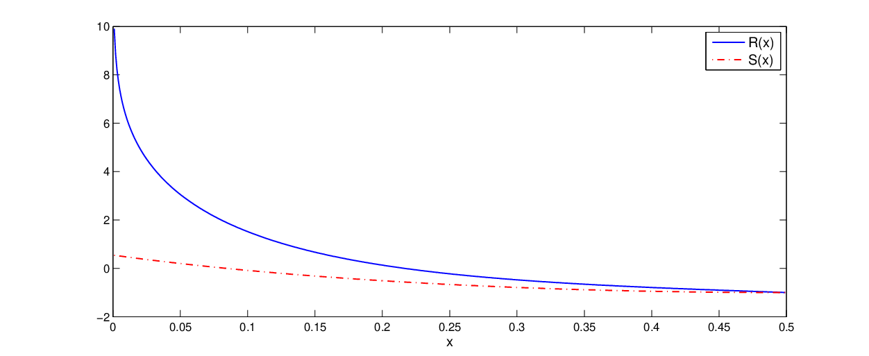
for all 16≤p≤12\frac{1}{6}\leq p\leq\frac{1}{2} and x∈[0,12]x\in[0,\frac{1}{2}]. Given any x∈[0,12]x\in[0,\frac{1}{2}], observe that J⁡(x∗p)​(1−2​(x∗p))J(x*p)(1-2(x*p)) is a decreasing function of pp for 0≤p≤120\leq p\leq\frac{1}{2}. Thus establishing (4) for p=16p=\frac{1}{6} suffices.

Let S⁡(x)=−1+J⁡(x∗16)​(1−2​(x∗16))S(x)=-1+J(x*\frac{1}{6})(1-2(x*\frac{1}{6})). Figure 3 plots S⁡(x)S(x) and R⁡(x)R(x).

Refer to caption
Fig. 3: Comparing R⁡(x)R(x) and S⁡(x)S(x)

Thus we have S⁡(x)≤R⁡(x)S(x)\leq R(x) for 0≤x≤120\leq x\leq\frac{1}{2}. This completes the proof of Claim 1.