Hiding Under the Carpet: a New Strategy for Cloaking

Jensen Li, J. B. Pendry Affiliation: Blackett Laboratory, Imperial College London, London SW7 2AZ

Abstract

A new type of cloak is discussed: one that gives all cloaked objects the appearance of a flat conducting sheet. It has the advantage that none of the parameters of the cloak is singular and can in fact be made isotropic. It makes broadband cloaking in the optical frequencies one step closer.

pacs

42.79.-e, 02.40.-k, 41.20.-q

Transformation optics [1, 2, 3, 4] can be used to design a cloak of invisibility. In essence the cloak makes its contents appear to be very small and hence invisible. However there are three distinct topological possibilities: the cloaked object can be crushed to a point, to a line, or to a sheet. In the process of crushing the object becomes infinitely conducting but this does not present a problem for the first case because scattering from even highly conducting small objects vanishes with the size of object. The same is true of a very thin object, i.e. a wire, because very thin wires have very large inductance and are therefore invisible to radiation. This is not true of the third possibility. Obviously a conducting sheet is highly visible unless of course it sits on another conducting sheet (the ‘carpet’ of the title). Although this third possibility has limited cloaking potential it does have the considerable advantage that the parameters of the cloak need not be singular and, as we shall show, can be isotropic.

Metamaterials are usually used as the building blocks for transformation optics as they can attain a wide range of permittivity and permeability. Several works investigated the cylindrical cloak in full wave analysis and the first experiment in verifying the cloak is done in microwave. [5, 6, 7, 8] There are other approaches targeting the subwavelength regime [9, 10] and the geometrical optics regime [11] for cloaking as well. Here, we concentrate on the transformation optics approach which is driven by coordinate transformation and has a large variety of applications.[12, 13]

There is still a general quest to push the working frequency to visible regime for more applications. However, scaling down the magnetic resonating structures for the metamaterials to optical frequencies causes severe absorption. [14, 15, 16, 17, 18] One way to avoid it is to use the reduced material parameters in the cloak so that only anisotropic metamaterials with electric resonating elements are needed. [19] However, as long as we are using metamaterials with resonating structures, materials absorption still cannot be neglected.

In this work, instead of the complete cloak, we will consider a cloak to mimic a flat ground plane. We will show that it does not require singular values for the material parameters, i.e. the range for the permittivity and the permeability is much smaller than in the case of a complete cloak. Moreover, by choosing a suitable coordinate transform, the anisotropy of the cloak can be minimized to a small value also. As a result, we can avoid using metamaterials and just use isotropic dielectrics to construct the cloak. It greatly reduces absorption and also make broadband cloaking one step closer.

Here, we consider only the 2D wave problem for simplicity, i.e. all the fields are invariant in the z-direction. Furthermore, the E-polarization is assumed while the formulation can be easily adopted for the other polarization. A ground plane here means a highly reflecting surface made of metal. It is regarded as a perfect conductor. Suppose an object lies on it, we want to design a cloak covering on the object so that the observer perceives the system as a flat ground plane again without introducing any additional scattering from the object. The object is now concealed between the cloak and the original ground plane as shown on the left hand side of Fig. 1. We further assume that the cloak (shown in cyan color) has a rectangular shape of a width of $w$ and a height of $h$ except that the bottom (inner) cloak boundary is curved upwards to leave enough space to conceal the object. The whole configuration is termed as the physical system with coordinate $\left({x,y}\right)$ or literally written as $\left({x^{1},x^{2}}\right)$ in indexed notation. The virtual system is the configuration the observer perceives. It is shown on the right hand side of Fig. 1. Its coordinate is labeled by $\left({\xi,\eta}\right)$ or literally written as $\left({\xi^{1},\xi^{2}}\right)$ in indexed notation. In general, we are considering a coordinate transform which maps (with sense preserving) a rectangular region ( $0\leq\xi\leq w$ , $0\leq\eta\leq h)$ in the virtual system to an arbitrary region (the cloak in this case) in the physical system.

Refer to caption — Figure 1: (color online). The general mapping between the virtual system and the physical system. The regions in cyan color are transformed into each other. The shaded region at the bottom of both domain represents the ground plane (a perfect conductor). The observer perceives the physical system (x-system) as the virtual system with a flat ground plane.

To ease our discussion, we introduce the Jacobian matrix $\Lambda$ by

\Lambda^{i}_{i^{\prime}}=\frac{\partial x^{i}}{\partial\xi^{i^{\prime}}},

(1)

and the covariant metric $g$ by

g_{{i}^{\prime}{j}^{\prime}}=\vec{\xi}_{i}^{\prime}\cdot\vec{\xi}_{j}^{\prime}\quad\mbox{or}\quad g=\Lambda^{T}\Lambda,

(2)

where $\vec{\xi}_{1}$ , $\vec{\xi}_{2}$ are the covariant basis vectors of the virtual coordinates appearing in the physical system. In the application of cloaking, the observer perceives the physical system as the virtual system of an isotropic homogeneous medium of permittivity $\varepsilon_{\mbox{ref}}$ and unit permeability. The corresponding permittivity and permeability in the physical system induced by the coordinate transformation are given by

\begin{array}[]{l}\varepsilon=\varepsilon_{ref}/\sqrt{\det g},\\ \left[{\mu^{ij}}\right]=\frac{1}{\sqrt{\det g}}\Lambda\Lambda^{T}.\end{array}

(3)

We can write $\mu_{T}$ and $\mu_{L}$ be the principal values of the matrix representation of the permeability tensor in the physical domain and the corresponding refractive indices be $n_{T}=\sqrt{\mu_{L}\varepsilon}$ and $n_{L}=\sqrt{\mu_{T}\varepsilon}$ for the two (local) plane waves traveling along the two principal axes. To indicate the extent of anisotropy of the physical medium, the anisotropy factor $\alpha$ (a function of position) is defined by

\alpha=\max\left({n_{T}/n_{L},n_{L}/n_{T}}\right).

(4)

By using Eq. (3) and Eq. (2), it can be proved that

\alpha+\frac{1}{\alpha}=\frac{Tr\left(g\right)}{\sqrt{\det g}},

(5)

with

\mu_{L}\mu_{T}=1.

(6)

On the other hand, we can define an averaged refractive index $n$ relative to the reference medium by

n=\sqrt{n_{L}n_{T}}/\sqrt{\varepsilon_{ref}},

(7)

so that

n^{2}=\frac{\varepsilon}{\varepsilon_{ref}}=\frac{1}{\sqrt{\det g}}.

(8)

Instead of using $\varepsilon$ and $\mu^{ij}$ to describe the physical medium, we now use $\alpha$ and $n$ (related to the ratio and the product of $n_{T}$ and $n_{L})$ which have geometrical meanings in terms of the metric. If we imagine there is a very fine rectangular grid in the virtual domain with every tiny cell being a square, the mapping (or the coordinate transform) transforms this grid to another grid in the physical domain. Every such tiny square ( $\delta\times\delta)$ in the virtual domain is transformed to a parallelogram with two sides $\vec{\xi}_{1}\delta$ and $\vec{\xi}_{2}\delta$ . A smaller anisotropy means a smaller value of $Tr\left(g\right)/\sqrt{\det g}$ while a smaller area of the transformed cell ( $\sqrt{\det g}\delta^{2})$ means a larger refractive index $n$ .

In cloaking, compression of space in the physical domain essentially makes the cloak anisotropic. However, our heuristic approach is to minimize the anisotropy induced in the physical medium by choosing a suitable coordinate transform. If the anisotropy is small enough, we can simply drop this part (by assigning $\alpha=1$ ) and only keep the refractive index $n$ . In other words, the physical medium becomes just a dielectric profile described by Eq. (8) with unit magnetic permeability.

In this work, such an optimal map is generated by minimizing the Modified-Liao functional [20]

\Phi=\frac{1}{hw}\int_{0}^{w}{d\xi}\int_{0}^{h}{d\eta}\frac{Tr\left(g\right)^{2}}{\det g},

(9)

upon slipping boundary condition. Slipping boundary condition means that each of the four bounding edges of the virtual domain must be mapped to the four specified boundaries in the physical domain, only up to a sliding freedom. The minimal of this functional occurs at the quasiconformal map [21]. Without going further for technical proof, we state the result that the quasiconformal map actually minimizes not only the average but also the maximum value of $Tr\left(g\right)/\sqrt{\det g}$ in the physical domain, i.e. anisotropy minimized. If we imagine there is a very fine rectangular grid in the virtual domain with every tiny cell being a square, the transformed grid in the physical domain for the quasiconformal map has the property that every transformed cell is a rectangle of a constant aspect ratio $M:m$ where $M$ is called the conformal module of the physical domain (a geometrical property of the physical domain once the four boundaries are specified) and $m=w/h$ is the conformal module of the virtual domain, i.e.

\frac{\left|{\vec{\xi}_{1}}\right|}{\left|{\vec{\xi}_{2}}\right|}=\frac{M}{m},\quad\sqrt{\det g}=\left|{\vec{\xi}_{1}}\right|\left|{\vec{\xi}_{2}}\right|.

(10)

By substituting Eq. (10) into Eq. (5), we have

\frac{Tr\left(g\right)}{\sqrt{\det g}}=\frac{M}{m}+\frac{m}{M},\;\quad\mbox{or}\quad\alpha=\max\left({\frac{M}{m},\frac{m}{M}}\right),

(11)

independent of position.

As a first example, let us map the area of a rectangle bounded by $0\leq\xi^{1}\leq 4$ , $0\leq\xi^{2}\leq 1.5$ in the virtual domain to the same rectangle in the physical domain but with the bottom boundary specified by

y_{\mbox{bottom}}\left(x\right)=\left\{{{\begin{array}[]{*{20}c}{0.2cos(\pi x/2)^{2}}\hfill&{1\leq x\leq 3,}\hfill\\ 0\hfill&{\mbox{otherwise}.}\hfill\\ \end{array}}}\right.

(12)

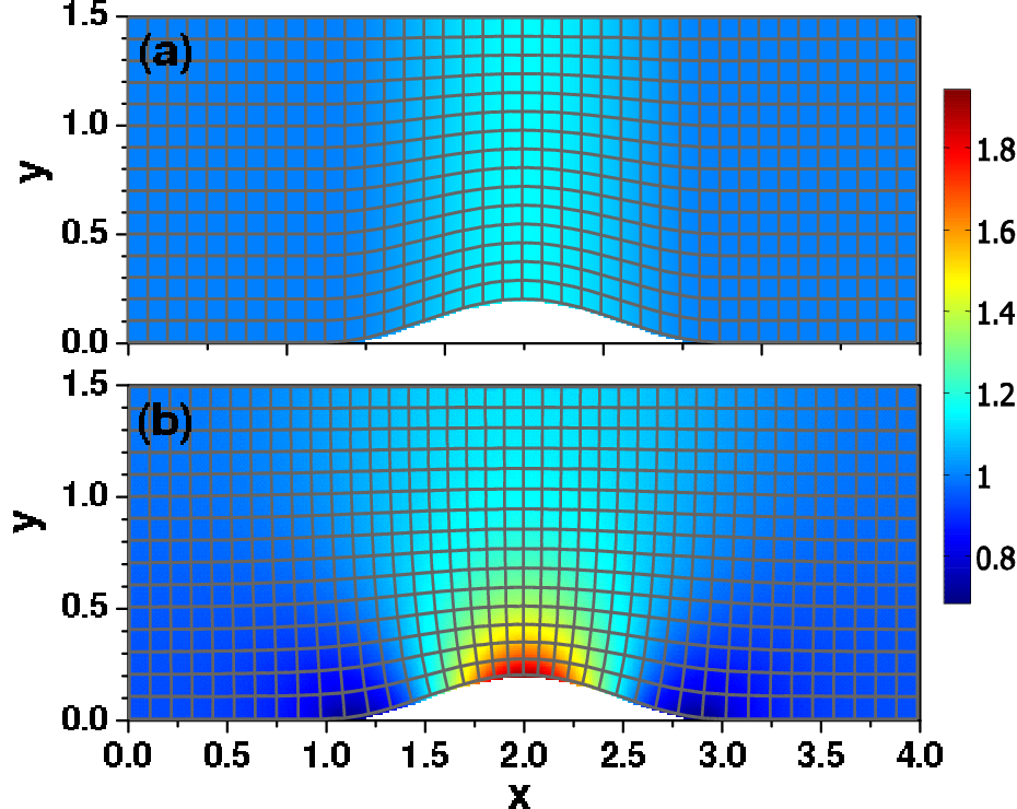
The transformed area in the physical domain is exactly the region of the cloak. Fig. 2(a) shows the transformed grid in the physical system if a simple transfinite interpolation is used to map a regular $40\times 15$ grid in the virtual domain. In this case, the grid is just a linear compression in the $y$ -direction. The corresponding range of the anisotropy factor $\alpha$ , obtained from Eq. (5), ranges from $1$ to $1.385$ while $n^{2}$ , obtained from Eq. (8), ranges from $1.0$ to $1.153$ . On the other hand, for the generated grid using quasiconformal map, shown in Fig. 2(b), the grid lines are orthogonal to each other. The aspect ratio of each cell or the anisotropy factor $\alpha$ becomes a constant of $1.042$ while $n^{2}$ ranges from 0.68 to 1.96. As the area of each cell is proportional to the square reciprocal of $n$ , the minimum of $n$ occurs on the inner cloak boundary at around $x=1$ where the cell area is largest while the maximum occurs also on the inner cloak boundary at $x=2$ where the cell area is smallest. Therefore, we sacrifice $n$ to a larger range at the same time anisotropy is minimized. Nevertheless, $n$ or $\varepsilon$ is always finite without approaching either zero or infinity. It is the result of crushing the object to a conducting plane instead of a line so that there is no singular point in the coordinate transform. The small anisotropy together with the finite range of $n$ makes realization of the cloak easier.

To test the effectiveness of the designed cloak, suppose the cloak is $4{\mu}m$ by $1.5{\mu}m$ , i.e. the length unit in the forehead discussion is in ${\mu}m$ and the $n$ profile given before is defined relative to silica glass ( $SiO_{2}$ ) of $\varepsilon_{ref}=2.25$ . We ignore the anisotropy in the cloak and only keep the part of permittivity. In this case, the permittivity of the cloak varies from around $1.5$ to $4.4$ . This range of permittivity can be obtained effectively by etching or drilling subwavelength holes of different sizes along the direction of E-field in a high dielectric, e.g. Si. Outside the cloak, it is again the silica glass as background material. Moreover, the inner surface of the cloak is coated by a highly reflective metal. To the observer, it is perceived as if this is the actual ground plane. This is relevant to the situation of routing light at our own will in optical integrated circuits. Suppose a Gaussian beam at a wavelength of 750nm (i.e. 500 nm in $SiO_{2}$ ) is launched at an angle of 45 degrees to the object together with the cloak, the total E-field pattern (real part) obtained from a FDTD simulation is shown in Fig. 3(a). The cloak is within the rectangle in dashed line in the figure. The field outside the cloak resembles the field as if we only have a flat ground plane. A reflected beam at 45 degrees is clearly seen. Moreover, the field inside the cloak shows the interference pattern between the incident and the reflected beam. The pattern is simply squeezed upwards if it is compared to the field when only a flat ground plane is present. The corresponding E-field pattern with only the object present is also shown in Fig. 3(b) for comparison. Without the cloak, the incident beam is deflected and split into two different angles. Therefore, our designed cloak successfully mimics a flat ground plane.

We emphasize that our strategy is valid in both geometrical and wave optics. In fact, it is broadband in nature. Our design works for a wide range of frequencies since the frequency dispersion (and also the losses) of the dielectrics can be made very small. For example, we can launch a Gaussian wave packet centered at the aforementioned frequency to the object and the cloak. The transverse width of the packet is set to $2{\mu}m$ with a duration of $20fs$ (8 periods of central frequency). It results an incident packet with circular spatial profile at time $t=0$ , as shown in Fig. 4(a). It is traveling at 45 degrees towards the object. After a duration of 14.8 periods at $t=37fs$ , the packet is reflected back at 45 degrees and it remains the same size of the Gaussian shape with only a small distortion (or dispersion) as shown in Fig. 4(b). This is certainly a time-domain cloaking effect. For comparison, we have also shown the field pattern at $t=37fs$ if the cloak is absent in Fig, 4(c). The incident wave packet is split into two elongated packets. There is nearly no distortion for the reflected wave packet in Fig. 4(b). However, if a thinner cloak or bigger object is used, it is expected that the distortion will become larger. It is due to a larger anisotropy neglected in our cloak profile.

In conclusion, a cloak is designed to mimic a flat ground plane. The involved coordinate transform induces no singular values in the material profile. Moreover, the quasiconformal map is the optimal coordinate transform which can minimize the anisotropy of the physical medium. The small anisotropy is further neglected so that the cloak can be synthesized by only isotropic dielectrics. It can relieve the loss issue by avoiding the usage of resonating elements and is a step closer to do broadband transformation optics in optical frequencies. The quasiconformal map should also be a convenient technique for both polarizations as well and in other applications in transformation optics.

This work is supported by the Croucher Foundation fellowship from Hong Kong.

References

[1] A. J. Ward and J. B Pendry, J. Mod. Opt. 43, 773 (1996).
[2] D. Schurig, J. B. Pendry and D. R. Smith, Opt. Express 14, 9794 (2006).
[3] J. B. Pendry, D. Schurig and D. R. Smith, Science 312, 1780 (2006).
[4] D. Schurig, J. J. Mock, B. J. Justice, S. A. Cummer, J. B. Pendry, A. F. Starr, D. R. Smith, Science 314, 977 (2006).
[5] S. A. Cummer, B. I. Popa, D. Schurig, D. R. Smith and J. B. Pendry Phys. Rev. E 74, 036621 (2006).
[6] F. Zolla, S. Guenneau, A. Nicolet and J. B. Pendry, Opt. Lett. 32, 1069 (2007).
[7] Z. Ruan, M. Yan, C. W. Neff and M. Qiu, Phys. Rev. Lett. 99, 113903 (2007).
[8] B. Zhang, H. Chen, B. Wu, Y. Luo, L. Ran, and J. Kong, Phys. Rev. B 76, 121101 (2007).
[9] A. Alu and N. Engheta, Phys. Rev. E 72, 016623 (2005).
[10] G. W. Milton and N.-A. P., Nicorovici, Proc. R. Soc. A 462, 3027–3059 (2006).
[11] U. Leonhardt, Science 312, 1777 (2006).
[12] M. Rahm, D. Schurig, D. A. Roberts, S. A. Cummer, D. R. Smith, J. B. Pendry, arXiv:0706.2452v1
[13] H. Chen and C. T. Chan, App. Phys. Lett. 90, 241105 (2007).
[14] Stefan Linden, et. al., Science 306, 1351 (2004).
[15] V M Shalaev, et. al., Opt. Lett. 30, 3356 (2005).
[16] S. Zhang, et. al., Opt. Express 13, 4922 (2005).
[17] G. Dolling, et. al., Opt. Lett. 31, 1800 (2006).
[18] G. Dolling, et. al., Opt. Lett. 32, 53 (2007).
[19] W Cai, et. al., Nature Photonics 1, 224 (2007).
[20] P. Knupp and S. Steinberg, Fundamentals of Grid Generation (CRC Press, 1994).
[21] J. F. Thompson, B. K. Soni and N. P. Weatherill, Handbook of Grid Generation (CRC Press, 1998).