A refinement of the Gribov-Zwanziger approach in the Landau gauge: infrared propagators in harmony with the lattice results
Abstract
Recent lattice data have reported an infrared suppressed, positivity violating gluon propagator which is nonvanishing at zero momentum and a ghost propagator which is no longer enhanced. This paper discusses how to obtain analytical results which are in qualitative agreement with these lattice data within the Gribov-Zwanziger framework. This framework allows one to take into account effects related to the existence of gauge copies, by restricting the domain of integration in the path integral to the Gribov region. We elaborate to great extent on a previous short paper by presenting additional results, also confirmed by the numerical simulations. A detailed discussion on the soft breaking of the BRST symmetry arising in the Gribov-Zwanziger approach is provided.
I Introduction
As is well known, quantum chromodynamics (QCD) is confining at low energy. Confinement means that it is impossible to detect free quarks and gluons in the low momentum region as quarks form colorless bound states like baryons and mesons. Even if one omits the quarks, pure Yang-Mills gauge theory remains confining as gluons form bound states known as glueballs. Hitherto, confinement is still poorly understood. There is a widespread belief that the infrared behavior of the gluon and ghost propagator is deeply related to the issue of confinement and, therefore, these propagators have been widely investigated. In this paper, we shall use the following conventions for the gluon and the ghost propagator,
| (1) |
Until recently, lattice results have shown an infrared suppressed, positivity violating gluon propagator which seemed to tend towards zero for zero momentum, i.e. , and a ghost propagator which was believed to be enhanced in the infrared [2, 1], with . Different analytical approaches were in agreement with these results (e.g. [3, 4, 5, 6, 7, 8, 9, 10]) to quote only a few). For instance, several works based on the Schwinger-Dyson or Exact Renormalization Group equations reported an infrared enhanced ghost propagator and an infrared suppressed, vanishing gluon propagator, obeying a power law behavior characterized by a unique infrared exponent, as stated by a sum rule discussed in [3, 4, 5, 6]. The infrared propagators have also been studied from a thermodynamical viewpoint in [11]. Also the Gribov-Zwanziger action predicts an infrared enhanced ghost propagator and a zero-momentum vanishing gluon propagator [8, 9]. This action was constructed in order to analytically implement the restriction to the Gribov region , defined as the set of field configurations fulfilling the Landau gauge condition and for which the Faddeev-Popov operator,
| (2) |
is strictly positive, namely
| (3) |
The boundary, , of the region is called the (first) Gribov horizon. This restriction is necessary to avoid the appearance of Gribov copies in the Landau gauge related to
gauge transformations [7]. However, this region still contains a number of Gribov copies and is therefore still “larger” than the fundamental modular region (FMR), which is completely free of Gribov copies. Unfortunately, it is unknown how to treat the FMR analytically [12, 13, 14, 15].
However, more recent lattice data
[18, 16, 17, 19]
at larger volumes display an infrared suppressed, positivity
violating gluon propagator, which is nonvanishing at zero
momentum, , i.e. , and a ghost propagator which is no longer
enhanced, . This implies that the previous mentioned analytical
approaches are not conclusive. It is worth pointing out that,
recently, the authors of [20, 21] have
obtained a solution of the Schwinger-Dyson equations which is in
agreement with the latest lattice data. Furthermore, as we have
shown in a previous work [22], this agreement can
also be found within the Gribov-Zwanziger approach. In this
framework, we have added a novel mass term to the original
Gribov-Zwanziger action. This new term corresponds to the
introduction of a dimension 2 operator. We recall that by
including condensates, which are the vacuum expectation value of
certain local operators, one can take into account nonperturbative
effects which play an important role in the infrared region.
During the course of the current work, it shall become clear that
we also have to add an additional vacuum term to
the action, which will allow us to stay within the Gribov
region . The previous paper
[22] only gave a brief account of the consequences
of adding the mass operator to the original Gribov-Zwanziger
action. For this reason, here we shall present an extensive study
of the Gribov-Zwanziger action with
the inclusion of the new parts.
The purpose of this paper is fourfold, and it is organized as follows. The first aim, discussed in section II, is to give a detailed proof of the renormalizability of the extended action. Therefore, we first present an overview of the Gribov-Zwanziger action, , in the Landau gauge which implements the restriction the Gribov region . Next, we add the local composite operator to this action and we prove the renormalizability of this extended action, . Subsequently, we show that by adding another term, , the renormalizability is not destroyed. In summary, section II establishes the renormalizability of the action . The second aim, investigated in section III, is to demonstrate that this extra term enables us to obtain propagators which exhibit the desired behavior. In particular, the tree level gluon propagator is calculated explicitly and the ghost propagator is determined up to one loop. Both the ghost and the gluon propagator are in qualitative agreement with the latest lattice results. Up to this point, we have added this mass term by hand. Hence, a third aim is to obtain a dynamical value for . Section IV presents this dynamical value. An estimate for the one loop gluon propagator at zero momentum as well as for the ghost propagator at low momenta is given. Also, the positivity violation of the gluon propagator is scrutinized and compared with the available lattice data. The last aim is to highlight the BRST breaking of the Gribov-Zwanziger action, which is presented in detail in Section V. We already stress here that it is the restriction to the Gribov region , implemented by the Gribov-Zwanziger action, which induces the explicit breaking of the BRST symmetry. Further, we provide a few remarks on the Maggiore-Schaden approach to the issue of the BRST breaking [23], and we revisit a few aspects of the Kugo-Ojima confinement criterion [24]. We end this paper with a discussion in section VI.
II The extended action and the renormalizability
II.1 The Gribov-Zwanziger action
We begin with an overview of the action constructed by Zwanziger [10] which implements the restriction to the Gribov region [7] in Euclidean Yang-Mills theories in the Landau gauge. We start from the following action,
| (4) |
with the classical Yang-Mills action,
| (5) |
and the so called horizon function,
| (6) |
The parameter , known as the Gribov parameter is not free and is determined by the horizon condition:
| (7) |
where is the number of space-time dimensions. The nonlocal horizon function can be localized through a suitable set of additional fields. The complete localized action reads
| (8) |
with
| (9) |
The fields are a pair of complex conjugate bosonic fields, while are anticommuting fields. Each of these fields has components. We can easily see that the action displays a global symmetry, , with respect to the composite index , of the additional fields . Therefore, we simplify the notation of these fields by setting
| (10) |
so we get
| (11) |
Now we shall try to translate the horizon condition (7) into a more practical version [9]. The local action and the nonlocal action are related as follows,
| (12) |
If we take the partial derivative of both sides with respect to we obtain,
| (13) |
Using this last expression and assuming that , we can rewrite the horizon condition (7)
| (14) |
We know that the quantum action is obtained through the definition
| (15) |
where stands for the integration over all the fields. It is now easy to see that
| (16) |
is exactly equivalent with equation (14). Therefore, equation (16) represents the horizon condition. We
remark that the condition (16) also includes the solution . However, would correspond to the case in which the
restriction to the Gribov region would not have been implemented. As such, the value has to be disregarded as an artefact due to the reformulation of the horizon condition.
As it has been proven in [9], the Gribov-Zwanziger action is renormalizable to all orders. In the next section, we shall give an overview of this renormalizability, but with the insertion of the local composite operator , to extend the action further. Obviously, the renormalizability of this extended action also includes the renormalizability of the ordinary Gribov-Zwanziger action .
II.2 Adding the local composite operator
If we add the local composite operator to (8) one can prove [25] that the following action is renormalizable to all orders
| (17) |
with
| (18) |
with a new source and a new parameter. We now go a
little bit more into the details of the renormalization of this
action, as it will be useful later. We remark that
if we prove the renormalizability of the action , we have also
proven the renormalizability of just by
putting equal to zero. We will use the method of algebraic
renormalization [28]. Roughly speaking, this means that we will embed the action into a
larger action by adding new sources, so it will display a greater
number of symmetries. These symmetries are important as they will
imply constraints on the possible allowed
counterterm. The larger the number of symmetries, the more
limitations we will find on the counterterm. This will lead to a
bigger possibility to absorb the counterterm into the original
action, thereby proving the renormalizability. In the end, we give
the sources the correct physical values, so we obtain the
action again.
We shall now implement, step by step, this method of algebraic renormalization. Firstly, we introduce two local external sources , so we can treat and as composite operators just like . Hence, we replace the term by
| (19) |
If we set the sources to their physical values in the end
| (20) |
we obtain, as requested, the term defined in (8).
Secondly, the algebraic renormalization procedure
requires this action to be BRST invariant. Therefore, we further
introduce three extra sources , and
and replace by
| (21) | |||||
where the BRST transformations of all the fields and sources are:
| (22) |
and
| (23) |
We recall that the BRST operator is nilpotent, meaning that . We mention again that by replacing the sources with their physical values in the end
| (24) | |||
| (25) |
one recovers the original terms .
Finally, a term ,
| (26) |
was added, which is needed to define the nonlinear BRST transformations of the gauge and ghost fields. and are two new sources, invariant under the BRST symmetry and with
| (27) |
The enlarged action is thus given by
| (28) |
and one easily sees that the action is indeed BRST invariant. This action now enjoys a larger number of Ward identities summarized as follows:
| dimension | ||||||||
| dimension | ||||||||
| 0 | 0 | |||||||
| 0 | 0 |
- •
- •
The Slavnov-Taylor identity reads
(30) with
(31) - •
The Landau gauge condition and the antighost equation are given by
(32) (33) - •
The ghost Ward identity is
(34) with
and
(36) Notice that the term , being linear in the quantum fields , , is a classical breaking.
- •
The linearly broken local constraints yield
(37) (38) (39) (40) - •
The exact symmetry reads
(41) with
(42)
When we turn to the quantum level, we can use these symmetries to characterize the most general allowed invariant counterterm . Following the algebraic renormalization procedure [28], is an integrated local polynomial in the fields and sources with dimension bounded by four, and with vanishing ghost number and -charge. The previous Ward identities imply the following constraints for :
- •
The invariance:
(43) - •
The linearized Slavnov-Taylor identity:
(44) with the nilpotent linearized Slavnov-Taylor operator,
(45) and
(46) - •
The Landau gauge condition and the antighost equation:
(47) - •
The ghost Ward identity:
(48) - •
The linearly broken local constraints:
- •
The exact symmetry:
(49)
These constraints imply that does not depend on the Lagrange multiplier , and that the antighost and the -valued fields , , , can enter only through the combinations [9, 25]
| (50) |
The most general counterterm fulfilling the conditions (43) - (49) contains four arbitrary parameters, , , , and reads
| (51) |
Once the most general counterterm has been determined, one can straightforwardly verify that it can be reabsorbed through a multiplicative renormalization of the fields, sources and coupling constants. We also mention the renormalization factors, useful for later calculations. If we set , , , , , , , for all the fields and , , , , , , for the sources, and if we define
| (52) |
one can determine
| (53) |
These are the only independent renormalization constants. For example, the Faddeev-Popov ghosts and the -valued fields have a common renormalization constant, determined by the renormalization constants and ,
| (54) |
The renormalization of the sources is also determined by the renormalization constants and , being given by
| (55) |
Also is related to and [25]:
| (56) |
Finally, , and are also not independent as they are given by:
| (57) |
II.3 Adding a new mass term
II.3.1 Extended action
We first explain the need for the inclusion of a new dynamical effect. According to the latest lattice results, the gluon propagator does not seem to vanish for zero momentum. This is incompatible with the actions (8) and (17), which both lead to a vanishing gluon propagator near the origin. The tree level gluon propagator in the Gribov-Zwanziger model reads [25]
| (58) |
where we have set
| (59) |
One recognizes indeed that expression (58) vanishes at the origin due to the presence of Gribov parameter . In the model the gluon propagator is modified in the following form,
| (60) |
which reveals a further suppression near the origin and thus it still vanishes. We recall here that the fields were introduced to localize the horizon function [9], which implements the restriction to the Gribov-region . If we take a closer look at the action (11), we observe an -coupling at the quadratic level. One can suspect that a nontrivial effect in the -sector will immediately get translated into the gluon sector. For this reason, if we try to give a mass to the -fields without spoiling the renormalizability of the action, we might be able to modify the gluon propagator in the desired way. Implementing this idea means that we add a new term to the action (17) of the form , with a new source. If we want to preserve the renormalizability we have to add the mass term in a BRST invariant way. Therefore, we consider the following extended action:
| (61) | |||||
| (62) | |||||
with a parameter and a dimension two source, invariant under the BRST transformation
| (63) |
II.3.2 Renormalizability
The proof of the renormalizability of this action can be easily done with the help of the Ward identities derived in the previous section. Again, we embed the action into a larger action,
| (64) |
containing more symmetries. It is subsequently trivial to check that all Ward identities (29)-(42) remain unchanged up to potential harmless linear breaking terms and therefore the constraints (43)-(49) as well as the combinations (50) are preserved. This implies that the counterterm corresponding to the action is now given by
| (65) |
with an arbitrary parameter. This counterterm can be absorbed into the original action , hence we have proven the renormalizability of our extended action. If we define
| (66) |
we find
| (67) |
As the reader might have noticed, symmetries do also not prevent a term to occur, with a new parameter, but we can argue that is in fact a redundant parameter, as no divergences in will occur. A term of this form is independent of the fields, hence it would only be necessary to get rid of the infinities in the functional energy, which we calculate by integrating the action over all the fields
| (68) |
Seen from another perspective, we need a counterterm to remove possible divergences in the vacuum correlators for . Such new divergences are typical when a local composite operator (LCO) of dimension 2 is added to the theory in 4D. An a priori arbitrary new coupling is then needed to reabsorb these divergences. In general, it can be made a unique function of such that obeys a standard homogeneous linear renormalization group equation [25]. This is a good sign, as we do not want new independent couplings entering our action or results. A nice feature of the LCO under study, i.e. , is that divergences are in fact absent in the correlators, so there is even no need for the coupling here. The argument goes as follows. The Ward identitites prohibit terms in from occurring. Notice that this is not a trivial point, as naively we expect it to occur from the dimensional point of view. It is only by making use of the extended action and its larger symmetry content that we can exclude a term from the game. Hence, we can set to find the vacuum divergence structure , as we will employ as usual mass independent renormalization schemes like the scheme. Now, there are two ways to understand that no divergences in will occur. Firstly, at the level of the action is easily recognized that the term in the action is irrelevant for the computation of the generating functional as the associated vertices cannot couple to anything without external - and -legs. Thus forgetting about this term, the - and -integrations can be done exactly, and they neatly cancel due to the opposite statistics of both sets of fields. Hence, all -dependence is in fact lost, and a fortiori no divergences arise. Secondly, for , the action is BRST invariant, . Consequently, the vacuum correlators . Therefore, we have again proven that no divergences in appear. For , the BRST transformation no longer generates a symmetry (see section V), hence a nonvanishing result for the correlator or the condensate is allowed. A nonvanishing VEV for our new mass operator is thus exactly allowed since the BRST is already broken by the restriction to the horizon. From the first viewpoint, the - and -integrations will no longer cancel against each other, giving room for -dependent contributions in the generating functional, albeit without generating any new divergences.
II.4 Modifying the effective action in order to stay within the horizon
II.4.1 Extended action
A very important fact is to check if it is still possible to stay within the Gribov region , after adding this new mass term. This can be investigated with the help of the ghost propagator , which can be easily read off from the Feynman diagrams depicted in FIG. 1,

| (69) | |||||
with
| (70) |
Going back to the original formulation of Gribov [7], being inside the region , is equivalent to state that
| (71) |
which is called the no-pole condition. In this case, the ghost propagator can be rewritten in the following form,
| (72) |
which represents the fact that we are working at the level of the inverse propagator or equivalently, at the level of the 1PI -point functions, which are generated by the effective action . This form is more natural, as we can now impose the gap equation (16), which is also formulated at the level of the effective action. However, in the next section, it shall become clear that the current action does not guarantee us that we are located within the region as . Therefore, we add a second term to the action, , given by
| (73) |
with a new parameter. We have introduced the particular prefactor of for later convenience. As it is a constant term, is it comparable with the term in the original Gribov-Zwanziger formulation (9). Therefore, it can be responsible for allowing us to stay inside the Gribov horizon by enabling to be smaller than 1. The explicit calculation of will be done in the next section, but we can already intuitively sketch the reasoning why will be altered. As this new term is independent of the fields, it will only enter the expression for the vacuum energy. However, due to the gap equation (16), it will also enter in the expression of the ghost propagator (and analogously any other quantity which contains ). Recapitulating, the complete action now reads,
| (74) |
with given in equation (61).
II.4.2 Renormalizability
The renormalizability of can be easily verified. Therefore, we replace with
| (75) |
with a color singlet and BRST invariant source, . In the end, we give the physical value of
| (76) |
to return to the original action . Again, we embed the action into a larger action ,
| (77) |
with given by (64). Firstly, as it is easily checked, the term can only give rise to an additional harmless classical breaking in the Ward identities. Therefore, all the previous Ward identities will remain valid. Secondly, we have the following additional Ward identity,
| (78) |
which implies that the counterterm is independent from . Taking these two argument together, we can conclude that the counterterm will be exactly the same as before, given by (65). Therefore,
| (79) |
and consequently, no new renormalization factor is necessary,
| (80) |
II.4.3 Boundary condition
Introducing a new parameter , requires a second gap equation in order to determine this new parameter. We recall that, in the case in which or equivalently in the original Gribov-Zwanziger formulation, we have
| (81) |
with a certain positive constant, which causes the enhancement of the ghost propagator at zero momentum,
| (82) |
Therefore, we know that at zero momentum, slowly switching off , will cause going to 1. It is therefore very natural to demand that this transition has to occur smoothly by imposing the following boundary condition,
| (83) |
In summary, we have now two gap equations. Firstly, the gap equation fixes as a function of and secondly, demanding that will uniquely fix . This leaves us with one free parameter, , the fixation of which shall be discussed in section IV.
III The modified gluon and ghost propagator
Now that we have constructed the action , by adding two additional terms and to the original Gribov-Zwanziger action, we investigate the gluon and the ghost propagator in detail. For the calculations, we have replaced the sources and with the more conventional mass notations resp. .
III.1 The gluon propagator
We shall first examine the tree level gluon propagator. In order to calculate this free gluon propagator we only need that part of the free action containing the -fields and the , -fields. This free action reads
| (84) |
where the limit is understood in order to recover the Landau gauge. The “” stand for the constant terms and and other terms in the ghost- and -fields irrelevant for the calculation of the gluon propagator. Next, we integrate out the - and -fields. As we are only interested in the gluon propagator, we simply use the equations of motion, and , which give
| (85) |
We use this result to rewrite ,
| (86) | |||||
The last step is explained with the following relation,
| (87) |
and we restrict ourselves to the color group throughout. We continue rewriting so we can easily read the gluon propagator
| (88) |
The gluon propagator can be determined by taking the inverse of and converting it to momentum space. Doing so, we find the following expression
| (89) | |||||
From this expression we can already make two observations:
- •
enjoys infrared suppression.
- •
, so the gluon propagator does not vanish at the origin. Even if we set we still find a nonvanishing gluon propagator, so we want to stress that this different result is clearly due to the novel mass term proportional to .
In section IV.2 we shall uncover a third property, namely that displays a positivity violation. Also this observation is in accordance with the latest lattice results [29].
III.2 The ghost propagator
The observation that does not qualitatively alter the
gluon propagator, will be repeated for the ghost propagator.
Henceforth, we set , which also improves the
readability of the paper. However, all calculations
could in principle be repeated with the inclusion of the mass .
We start with the expression for the ghost propagator. Substituting the expression of the gluon propagator, we find,
| (90) | |||||
where we have also used equation (59). As we are interested in the infrared behavior of this propagator, we expand the previous expression for small ,
| (91) | |||||
For later use, let us rewrite as
| (92) |
Notice that the first integral in the right hand side of equation (92) diverges while the second integral is UV finite in .
We continue with the derivation of the gap equations as we would like to write as a function of , i.e. , in expression (92). Firstly, we calculate the horizon condition (16) explicitly starting from the effective action. The one loop effective action is obtained from the quadratic part of our action
| (93) |
This time, the terms and have to be maintained, as they will enter the horizon condition. After a straightforward calculation the one loop effective action in dimensions yields,
| (94) |
Setting (see equation (59)), we rewrite the previous expression,
| (95) |
and apply the gap equation (16),
| (96) |
Secondly, we impose the boundary condition (83) in order to obtain an explicit value for . Instead of explicitly starting from expression (90) to fix , there is a much simpler way to find the corresponding . Therefore, we act with on the gap equation (96). Subsequently setting , gives
| (97) |
where we imposed (83). Proceeding, we find
| (98) |
which determines at the current order.
With the help of the latter two gap equations (96) and (98), we can rephrase the correction to the self energy of the ghost. Combining equation (92) and (96) we can write
| (99) |
From this expression, we can make several observations. Firstly, when , from the previous expression it immediately follows that
| (100) |
which gives back the ordinary Gribov-Zwanziger result [7, 8, 10, 25]. Indeed, from the previous expression, one derived that the ghost propagator,
is enhanced and behaves like , for . Secondly, when , we notice that the ghost propagator is no longer enhanced and behaves like as already found in [22], which is in qualitative agreement with the latest lattice results. This behavior is clearly due to the novel mass term . Thirdly, we see that the term in is crucial in order to obtain a which is smaller than 1. Omitting this term would result in in the case that . However, including this term, we can easily prove that . Indeed, taking expression (99) and replacing with the integral in (98), we find
| (101) | |||||
with , hence . At this point, we can really appreciate the role of the
novel vacuum term (73). It serves as a stabilizing
term for the horizon condition. Indeed, without the
term (73), we would end up outside of the Gribov
region for some , even for an infinitesimal11
1
Notice
that we must take to avoid unwanted tachyonic
instabilities. . In this sense, the action
constitutes a refinement of the original Gribov-Zwanziger action,
which is a smooth limiting case of .
For later use, we can evaluate the integral in expression (99) as it is finite. The explicit one loop value for yields
| (102) |
where we have substituted the value (98) for .
In summary, we have found a ghost propagator which is no longer enhanced. So far, we have fixed in function of and we have found a constant value for . However, we have not yet fixed . This will be the task of the next section.
IV A dynamical value for
Up to this point, we have only introduced the mass by hand, however it is recommendable to obtain a dynamical value for this parameter. We shall present two methods to find such a value. Firstly, we explain how to obtain a dynamical value for with the help of the effective action. However, as the calculations become too involved, we investigate a second method, the variational principle, and apply this to the ghost and gluon propagator, with more success.
IV.1 The effective action and the gap equations
We first explain the idea behind the method before going into detailed calculations. In the previous section we have derived the gluon propagator. We recall that the mass term does not qualitatively change the form of the gluon and ghost propagators, therefore we have put for our purpose. With , the tree level propagator (89) yields:
| (103) |
Expanding the mass as a series in , gives
| (104) |
We only need to consider , which is of order unity, as we are considering the tree level propagator. We know that at the end of our calculations we have to set our sources equal to zero, or . If we work at lowest order, this means we have to set (and the gluon propagator will not display the desired behavior). However, going one order higher gives:
| (105) |
The last equation might imply that is no longer equal to zero, and consequently, the tree level gluon propagator will attain the desired form. Let us elaborate further on this aspect.
IV.1.1 One loop effective potential
To implement the above-mentioned ideas, we shall first calculate the one loop energy functional. We start with the action (61), whereby setting is equivalent with putting . We replace the mass again with the source . In order to determine the one loop effective action, we first need the one loop energy functional which we obtain from the quadratic part of the action,
| (106) |
From the previous expression we find for ,
| (107) |
We shall work in the scheme, and use a notational shorthand:
| (108) |
whereby is defined in equation (59). Evaluating the integrals in gives
| (109) |
This calculation is explained in detail in the appendix.
As we have determined the energy functional , we can now calculate the one loop effective action via the Legendre transform of . If we define
| (110) |
then
| (111) |
represents the expectation value of the local composite operator, . The effective action is given by
| (112) |
or equivalently, as we prefer to work in the variable ,
| (113) |
Calculating by explicitly doing the inversion is a rather cumbersome task. In most cases one can perform a Hubbard-Stratonovich transformation to eliminate the term from the action and introduce a new field which couples linearly to . This greatly simplifies the calculation. However, in this case, it seems impossible to do such a transformation as a required term in is missing. Hence, there is no other option than to actually perform the inversion. In order to calculate this inversion, we shall limit ourself to constant and as we are mainly interested in the (space time) independent vacuum expectation value of the operator coupled to the source . This vacuum expectation value is given by
| (114) |
where represents the ordinary Gribov-Zwanziger action (8). As we already have calculated up to one loop is it straightforward to verify that
| (115) |
whereby we shortened the notation by putting . From the previous expression we find for the condensate
| (116) |
This is an important result, as it indicates that a nonzero
value for the Gribov parameter will result in a
nonvanishing condensate
even at the perturbative level.
We are now ready to compute the effective action up to one loop along the lines of [30]. The energy functional can be written
as a series in the coupling constant ,
| (117) | |||||
As a consequence, looking at the definition (110), we can write
| (118) | |||||
where corresponds to the th order in (regarding as of order unity). This is called the original series. The inverted series is defined as
| (119) | |||||
with the th order coefficient. Substituting (119) into (118) gives,
| (120) | |||||
By regarding as of the order unity and by comparing both sides of the last equation, one finds
| (121) | |||||
| (122) |
For the moment, as we are working at lowest order, we only need equation (121). We can invert this equation, so we find for :
| (123) |
meaning that we have to solve
| (124) |
for , so we can write
| (125) |
We immediately suspect that this inversion will not give rise to an analytical expression. Once we have found , we substitute this expression into the effective action,
| (126) |
At this point, as we have found an expression for the one loop effective action, we can implement two equations to fix and . Firstly, the minimization condition reads
| (127) |
and secondly, the horizon condition (16) can be translated as
| (128) |
We start with the first gap equation. Replacing by equation (113) leads to
| (129) |
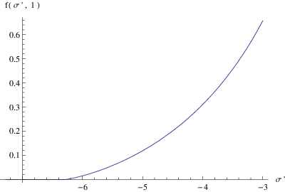
Since there are only 2 explicit scales, and , present, the first gap equation can be used to express e.g. in terms of . For the sake of a numerical computation, we can therefore momentarily set . From FIG. 2 one can obtain an estimate of , with . Doing so, we find , so that
| (130) |
which of course corresponds to the already obtained perturbative solution (116).
The second gap equation (128) must then consequently also give us back the perturbative solution. To check this, we first calculate the perturbative result for by taking the limit in expression (109)
| (131) |
Next, we take the partial derivative with respect to which gives,
| (132) |
The natural choice for the renormalization constant is to set to kill the logarithms. Imposing the gap equation gives us,
| (133) |
We remark that we have neglected the solution , as explained in section II.1. From
| (134) |
and expression (133) we find an estimate for :
| (135) |
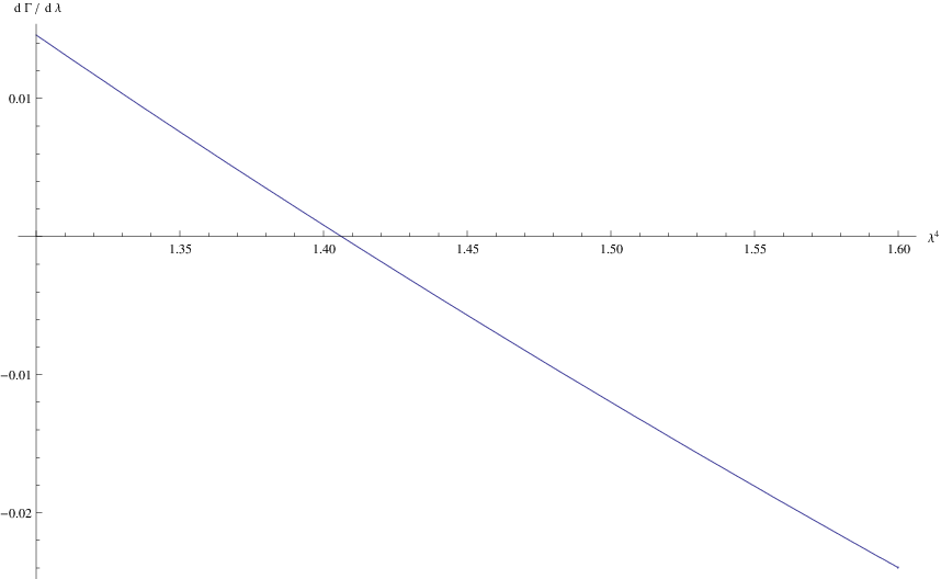
where we have worked in units . This perturbative solution is also in compliance with [25]. Now, we return to the effective action (126). We first take the partial derivative with respect to , afterwards we set , we explicitly replace by expression (134) and we use the minimizing condition (130). Numerically, we find the following value for :
| (136) |
as one can read off from FIG. 3. This is exactly the perturbative result (135).
If we calculate the vacuum energy with this value for , we find from (131),
| (137) |
We notice that the vacuum energy is positive.
IV.1.2 Intermediate conclusion
We can conclude at this point, that in the framework we have used, we recover only the perturbative solution. Unfortunately, at lowest order, one finds as explained in the beginning of this section, so we were unable to find a dynamical value for at first order. However, if we would be able to go one order higher, with , we might find and consequently the gluon propagator at tree level would attain the desired form (103). In addition, we might even discover a nonperturbative solution. Unfortunately, this is not as straightforward as at leading order. The main difficulty resides in the evaluation of two loop vacuum bubbles for the effective potential with three different mass scales. Whilst the master integrals are known, [31, 32, 33], the main complication is that the propagator of (89) with needs to be split into standard form but this introduces the masses of (108) which are either complex or negative. In either scenario the master two loop vacuum bubble is known for distinct positive masses and involves several dilogarithm functions. Therefore in our case for even the simplest of mass choices the resulting dilogarithms will be complex as well as being a complicated function of , and . Moreover, this is prior to computing the full effective potential itself by adding all the relevant combinations of master integrals together. Therefore, it seems to us that whilst such a computation could be completed in principle, currently the resulting huge expression could not possibly lend itself to a tractable analysis similar to the relatively simple one we have carried out at one loop.
IV.2 Applying the variational principle on the ghost propagator and the gluon propagator
In this section, we shall rely on variational perturbation theory in order to find a value for the hitherto arbitrary mass parameter
.
Along the lines of [34], we introduce a formal loop counting parameter by replacing the action with . At the same time, we replace all the fields by . Symbolically,
| (138) |
It is readily derived that multiplying each field with a factor of and performing an overall rescaling is the same as replacing the coupling with , so we can replace (138) with
| (139) |
In this fashion, the free (quadratic) part of the action is -invariant, while every interaction terms contains powers22
2
We recall that the perturbative expansion is one in powers of , and thus in integer powers of . of . The first order in the -expansion, obtained by setting , then corresponds to the free theory. More generally, the -expansion is equivalent with the loop expansion, where it is understood that we put the formal bookkeeping parameter at
the end.
The next step is to introduce the variational parameter into the theory. This is done in a specific way: we add the quadratic mass term to the action, but substract it again at higher order in , i.e. we consider the action
| (140) |
with . Since , we did not change the actual starting action at all.
However, we maintain the strategy of performing an expansion in powers of . Since the mass term is split up into 2 parts , both parts will enter the -expansion in a different way. At the end, we must set again. If we could compute an arbitrary quantity exactly, the -independence would of course be apparent since the theory is not altered. However, at any finite order in , a residual -dependence will enter the result for due to the re-expanded powers series in . Said otherwise, we have partially resummed the perturbative series for by making use of the parameter . The hope is that some nontrivial information, encoded by the operator coupled to , will emerge in the final expression for . One query remains: how to handle the which appears in the approximate ? Therefore we can rely on the lore of minimal sensitivity [35]: we know that the exact cannot depend on , hence it is very natural to demand that also at a finite order , leading to a dynamical optimal value for the yet free parameter .
The described method of variationally introducing extra parameters into
a quantum field theory provides us with a powerful tool to study nontrivial
dynamical effects in an approximate fashion, yet the calculational efforts
do not exceed those of conventional perturbation theory.
We still have to choose a value for . We recall that the constant term, , was introduced in order to stay within the horizon. Therefore, we want to retain this term when we are applying the variational principle. However, we are working up to first order, meaning that we shall expand the quantity up to first order in and subsequently set . Hence, taking is not a good option as the constant term would vanish and have no influence. Therefore, a better option is to take e.g. , to assure the consistency of the variational setup with the restriction to the Gribov region. In this way, we are simply coupling the variational parameter directly to the theory.
IV.2.1 The ghost propagator
We start from the expression (72) of the ghost propagator
| (141) |
and apply the variational principle on the ghost propagator near zero momentum. We have,
| (142) |
As explained above, we replace and . Subsequently, we expand in powers of corresponding to a re-ordered loop expansion. As we have calculated the ghost propagator up to one loop, we only need to expand the above expression to the first power of ,
| (143) |
As indicated earlier, setting gives
| (144) |
which is exactly the same as (142). This expression not only depends on , but also on . However, we already know that and are not independent variables, as they are related through the gap equation (96),
| (145) |
Following the variational principle, we replace with and with , expand the equation up to order , and set in the end. Doing so, we recover again expression (145). At this point, it can be clearly seen that in equation (140) would cancel the effect of the constant term , while is a better choice33 3 Actually, every value for , with is allowed.. Evaluating the integral in expression (145), we find
| (146) |
This integral could be similarly calculated as done in the appendix, or one could start from the effective action (126) and derive this equation with respect to . We recall that from the boundary condition (98), we have already determined .
We still require an appropriate value for . Therefore, we fix which was chosen as in [25]. We have opted for this specific renormalization scale which shall result in an acceptably small effective expansion parameter . Consequently, from equation (134), we find
| (147) |
in units of .
In summary, as remained the same after applying the variational principle, we can take the expression (102) for ,
| (148) | |||||
where is determined by the gap equation,
| (149) |
Before continuing the analysis, let us first have a look at the gap equation.
The gap equation solved for as a function of is
depicted in FIG. 4. We find two emerging branches, displayed
by a continuous and a dashed line. The former solution exists in the
interval , while the latter one only exists in . As
the latter branch does not exist around , we shall not consider this
solution because the boundary condition (83) demands a smooth
transition for the limit.

We can now have a closer look at the ghost propagator or equivalently . We have graphically depicted in FIG. 5. Firstly, from the figure, we see that is nicely smaller than 1 for all in the interval . This is a remarkable fact as it implies that we have managed to stay within the horizon. Secondly, we notice that the boundary condition is indeed fulfilled, which is a nice check on our result. We can now apply the minimal sensitivity approach on the quantity . From FIG. 5 we immediately see that there is no extremum. However, looking at the derivative of with respect to , we do find a point of inflection at . Demanding is an alternative option when no extremum is found [35]. Taking this value for , we find
| (150) |
The effective coupling is given by
| (151) |
which is smaller than 1.


IV.2.2 The gluon propagator
In order to apply the variational principle to the gluon propagator, we require its one loop correction. Given the rather complicated form of the propagator, obtaining the full exact expression for its one loop correction is not possible. Indeed to appreciate how cumbersome such an expression could be one has only to examine the case, [36], where all the one loop corrections to the propagators are given explicitly. However, despite this we can still achieve our main aim of studying the low momentum behavior of the gluon propagator corrections directly in the zero momentum limit without knowledge of the full correction. In [36] this limit for the gluon propagator was deduced from the exact one loop computation. However, the resulting expression tallied with that obtained via the vacuum bubble expansion of the underlying -point functions. The latter is a much easier technique to apply and given the equivalence of the expressions it justifies its application to our case when . Briefly one expands the -point functions relevant to the gluon propagator construction in powers of the external momentum . Though the expansion is truncated at some order such as . The accompanying Feynman integrals are massive vacuum bubbles which are essentially trivial to compute at one loop. However, our situation is complicated significantly by the fact that there is mixing in the quadratic part of the sector of the tree action. Therefore in addition to the gluon propagator, (70), we require the propagators of the remaining fields. For this derivation here we use the conventions and notation of the article [36] for an arbitrary color group, where the problem was discussed at length. There it is evident that one has to consider the full part of the momentum space action in order to invert the quadratic sector to derive all the propagators. In the Landau gauge we find the set of propagators for our situation are
| (152) |
where the presence of was a key ingredient in ensuring that ghost
enhancement correctly emerged in the case, [36].
Therefore we are confident that our extension here will include the previous
valid analysis and therefore will provide a useful check.
For the one loop propagator corrections one has to first compute the corrections to all the -point functions which were relevant for the derivation of (152). From [36] this is of the form
which is written with respect to the basis and as we work in the Landau gauge the common Lorentz structure, , has been factored off. The first matrix corresponds to the tree part of the action and the quantities , , , , , and represent the one loop corrections and we have used the shorthand coupling constant . The totally symmetric object is defined by, [37],
| (158) |
where is the adjoint representation of the color group generators. At this stage we note that (IV.2.2) represents a formal definition and no vacuum bubble expansion has been performed. To one loop one can formally invert (IV.2.2) to obtain the one loop corrections to all the propagators (152) which is
The objects , , , , , and are related to the quantities of the one loop matrix of (IV.2.2). However, as we are focussing in this article on the gluon propagator at zero momentum then we only need the relation for and note that the formal correction at one loop for this is
| (165) |
As noted above we could in principle compute the exact form of each of the
-point functions contributing to (165) but ultimately as we will
take the limit this would be unnecessarily
overcomplicated. Instead we compute those pieces of (165) which
remain at leading order in the vacuum bubble expansion.
For this we need to determine the fourteen contributing Feynman diagrams. These were generated using the Qgraf package, [38], and converted into Form input language where Form is a symbolic manipulation language, [39]. The vacuum bubble expansion written in Form was applied to each integral and expressions obtained for all the -point functions. As these depend on and we were able to check that our expressions agreed with those already determined in the , case of [36]. Moreover, we also checked the explicit Slavnov-Taylor identities for the renormalization of the new mass operator in the scheme by applying the Mincer algorithm, [40], written in Form, [41], to the Green’s function where the operator is inserted in an -point function. The resulting renormalization constants were crucial to not only ensuring that our conventions were consistent but also that our -point function vacuum bubble expansion is correctly finite after being fully renormalized. The upshot of our computations is the observation that for the gluon propagator in the zero momentum limit only is required for the leading (momentum independent) term of (165). Thus we finally obtain
| (166) | |||||
for the one loop correction at zero momentum where all mass
variables correspond to renormalized ones. We note that unlike the
case the nonzero freezing akin to tree order is
driven by the gluon -point function correction. By contrast in
the situation the gluon suppression at one loop
derives from the -point which is related to the horizon
condition and the gap equation. Also in this case will be
and not to retain suppression at one loop,
[36].
We apply the variational principle to the gluon propagator in a completely similar manner as in the case of the ghost propagator. Therefore, we replace with and with in the expression (166), expand up to order , and set . Doing so, we find the original expression (166) for the gluon propagator back. Firstly, we try to apply the principle of minimal sensitivity. Therefore, we have depicted the gluon propagator in FIG. 7. First, we notice that is positive for all . Unfortunately, we do find neither a minimum nor a point of inflection in this interval. Therefore, we shall take the value of , which was obtained in the study of the ghost propagator (see previous section). Hence, setting , gives
| (167) |
Evidently, the effective coupling is still smaller than 1, cfr. (151).

In summary, the infrared value of the ghost propagator and the zero momentum gluon propagator seem to be reasonable. We find a non-enhanced ghost propagator and a gluon propagator which is non-zero at zero momentum. Our results for the gluon and ghost propagator are of a qualitative nature as we are only working in a first order approximation. In order to improve these numerical results, higher order calculations are recommendable. This is however far beyond the scope of the present article.
IV.2.3 The temporal correlator: violation of positivity
With the help of the variational technique, we can also show that the gluon propagator displays a violation of positivity. If we rewrite the gluon propagator in the Källén-Lehmann spectral representation,
| (168) |
should be a positive function in order to interpret the fields in terms of stable particles. If for certain , is positivity violating. As a practical way to uncover this property, one defines the temporal correlator [2]
| (169) |
Consequently, if we can show that becomes negative for certain , cannot be positive for all , resulting in a positivity violating gluon propagator. If the gluon propagator vanishes at zero momentum, , one can immediately verify from (168) that cannot be a positive quantity. However, having , does not exclude a positivity violation as we shall soon find out.
We can now apply the variational technique on the temporal correlator. At tree level, this is given by
| (170) |
where is still determined by the gap equation (149). Replacing and is redundant in this case, as we only have the tree level gluon propagator at our disposal. We shall now implement the minimal sensitivity principle as follows: for each different value of , we minimize the temporal correlator with respect to . displays a minimum at , for . In TABLE 3, some values for for different are presented. For , we have taken ; it is clearly visible from the table below that for decreasing .
| 6 | 7 | 8 | 9 | 10 | |
|---|---|---|---|---|---|
| 0 | 0.16 | 0.35 | 0.51 | 0.65 |
The corresponding is depicted in FIG. 8. Both the -axis and -axis are shown in units fm ( fm), in order to compare our results with [29, 42]. Not only do we find a positivity violating gluon propagator as becomes negative, but even the shape of this function is consistent with the lattice results44 4 [29] included quarks, while [42] considered gluodynamics as we are studying in this work. [29, 42]. Moreover, in [29, 42], the positivity violation starts from fm, in good agreement with our results. Finally, FIG. 9 displays the corresponding values of . We can conclude that the previous results are reliable for as is smaller than one.


IV.3 A remark about the strong coupling constant
A renormalization group invariant definition of an effective strong coupling constant can be written down from the knowledge of the gluon and ghost propagators as
| (171) |
see e.g. [3]. and stand for the gluon and ghost form factor, defined by
| (172) |
The definition (171) represents a kind of
nonperturbative extension of the nonrenormalization of the ghost-gluon vertex. At the perturbative level, this is assured by the Ward identity (54), . Usually, this is assumed to remain valid at the nonperturbative level. Although this cannot be proven, this hypothesis has been corroborated by lattice studies like [44, 43].
In recent years, there was accumulating evidence that would reach an infrared fixed point different from zero: see e.g. [3, 4, 10, 5] for a Schwinger-Dyson analysis, [36, 45] in the ordinary Gribov-Zwanziger approach and [47, 46] for lattice results. These studies are mostly done in a MOM renormalization scheme, with the exception of [36] where the scheme was employed. The manifestation of this infrared fixed point was motivated in Schwinger-Dyson studies and the ordinary Gribov-Zwanziger case by means of the power law behavior of the form factors,
| (173) |
being expressable in terms of a single exponent . The Schwinger-Dyson community heralded in a variety of studies the value , whereas the Gribov-Zwanziger scenario gives . Anyhow, substituting a behavior like (173) into the definition (171) leads to , opening the door for a finite value.
However, once again quoting the more recent large volume lattice data of [16, 18, 43, 19], the power law behavior (173) seem to be excluded in favor of
| (174) |
leading to a vanishing infrared effective strong coupling constant at zero momentum since . The refined analysis in this paper of the extended Gribov-Zwanziger action, including an additional dynamical effect, allows us to draw a similar conclusion up to the one loop level, i.e. an infrared vanishing . Certain lattice studies also pointed towards this particular scenario [48].
V The BRST breaking in the Gribov-Zwanziger theory
We recall here that the Gribov-Zwanziger action (8) is not invariant under the BRST transformation (22). Indeed, if we take the BRST variation of the action (8), one finds a breaking term given by
| (175) |
We see that the presence of the Gribov parameter prevents
the action from being invariant under the BRST symmetry.
Nevertheless, this fact does not prevent the use of the
Slavnov-Taylor identity to prove the renormalizability of the
theory, which is very remarkable. Since the breaking
is soft, i.e. it is of dimension two in the
fields, it can be neglected in the deep ultraviolet, where we
recover the usual notion of exact BRST invariance as well as of BRST
cohomology for defining the physical subspace
[49]. However, in the nonperturbative infrared
region, the breaking term cannot be neglected and the BRST
invariance is lost. In the following, we shall present a detailed
analysis of this breaking and of its consequences. In particular, we
shall be able to prove that the origin of this breaking can be
traced back to the properties of the Gribov region .
Moreover, it turns out that the existence of this breaking enables
us to give an elementary algebraic proof of the fact that the Gribov
parameter is a physical parameter of the theory, entering
thus the expression of the correlation
functions of gauge invariant operators.
V.1 The transversality of the gluon propagator
The reader might wonder whether the gluon propagator still remains transverse in the presence of the Gribov horizon. As the gluon propagator is the connected two-point function, we ought to consider the generator of connected Green functions, which can be constructed from the quantum effective action55 5 This is the generator of the 1PI Green functions. by means of a Legendre transformation. The renormalizability of the theory entails that obeys the renormalized version of the Ward identity (32), or
| (176) |
Introducing sources for the fields and performing the Legendre transformation, the identity (176) translates into
| (177) |
Acting with on this expression, and by setting all sources equal to zero, we retrieve
| (178) |
which expresses nothing else but the transversality of the gluon propagator.
V.2 The BRST breaking and its consequences on the Slavnov-Taylor identity
Let us present here a few considerations on the consequences stemming from the BRST breaking appearing in the left hand side of equation (175) of the Slavnov-Taylor identity. Our argument will follow [50]. We start from the generalized Slavnov-Taylor identity (31) which is fulfilled by the enlarged action (28). The quantum effective action, , obeys the quantum version of this Slavnov-Taylor identity [28],
| (179) |
We now pass to the Gribov-Zwanziger action, defined by giving the sources (, , , ) their physical values (20) and (24). As a consequence, the physical quantum effective action will now obey a broken Slavnov-Taylor identity,
| (180) | |||||
whereby represents the generator of the 1PI Green functions with the insertion of the composite operator . Expression (180) generalizes at the quantum level the broken identity of equation (175). Once having a Slavnov-Taylor identity like (180) at our disposal, we can obtain relations between different Green functions by acting on it with test operators , with any field, and by setting all fields and sources equal to zero at the end. The breaking term in the r.h.s. of expression (180) will be translated into an extra contribution. In particular, we shall obtain
| (181) |
One sees thus that the r.h.s. of the foregoing expression,
corresponding to
a 1PI Green function with the insertion of the composite operator and with amputated external legs of the type
, gives precisely the modification of
the relationships among the Green functions due to the Gribov
horizon. To our understanding, the contributions stemming from the
r.h.s. of equation (181) should be correctly taken into account
when checking the validity of the Slavnov-Taylor identities or when
invoking Slavnov-Taylor related identities in computations when the
restriction to the Gribov horizon is
understood.
It is worth noticing that the breaking term of (181) will
certainly vanish if the chain has a
ghost number different from . Indeed, the action preserves ghost
number and the breaking term itself carries a
nonvanishing ghost charge of , so that the operator
must
have ghost number in order to allow for a nonvanishing contribution (181).
In summary, we emphasize that the broken Slavnov-Taylor identity (180) does in fact maintain a powerful predictive character. It allows us to establish relationships among various Green functions of the theory in a way which takes into account the presence of the Gribov horizon. At the same time, there exist Green functions for which the breaking of the Slavnov-Taylor identity is harmless. In particular, this is the case when considering gauge invariant operators built up with only the gauge fields . For these Green functions, the physical quantum action behaves as it fulfills the unbroken Slavnov-Taylor identity, namely
| (182) |
The gauge invariance of the correlator
implies in fact that no useful information can be extracted for it
from the Slavnov-Taylor identities. In a loose way of speaking,
lives on its own and is not related to
other Green functions. To formally prove this, one should add the
operator to the action with a (BRST invariant) scalar
source , the (broken) Slavnov-Taylor identity (180)
will remain unchanged. Hence, similarly as in the previous
subsection, by performing a Legendre transformation to pass to
and by acting with on that identity
and again setting all sources to zero, it will follow that there is
a trivially vanishing breaking term due to ghost charge
conservation.
V.3 A few words on unitarity
Certainly, the BRST breaking and its consequences on the Green
functions of the theory deserve further investigation. In this
respect one could attempt to evaluate some gauge invariant
correlation function like, for instance,
in order to see if, despite the presence of the BRST breaking and of
a positivity violating gluon propagator, this gauge invariant
correlation function might displays a real pole in momentum space. A
first hint that something like this might happen, has been given by
a tree level computation in
[8].
As one can easily figure out, the presence of the BRST breaking is related to the lack of unitarity in the gluon sector. To our understanding, this is a manifestation of gluon confinement: unitarity is jeopardized in the gluon sector because gluons are confined. This is also apparent from the positivity violation exhibited by the gluon propagator, which does not allow for a physical interpretation of the elementary gluon excitations. One might have the tendency to believe that the existence of the soft breaking of the BRST symmetry is a welcome feature, in particular signalling that, in a confining theory, physics in the infrared region is not necessarily definable in the same way as in the deep ultraviolet, where the BRST breaking could be neglected and one recovers usual perturbation theory. As we already stated in the beginning of this section, in the ultraviolet, we also recover the usual notion of the BRST cohomology [49], allowing to prove that the ghost degrees of freedom cancel against 2 unphysical gluon polarizations, leaving over only 2 physical transverse polarizations, endowed with a positive norm. In the confining regime, it is unknown what the analogue of this scenario might be. The absence of the BRST symmetry in the infrared does not necessarily entail that the theory is not unitary. Certainly, the -matrix of the excitations of the physical spectrum has to be unitary. But as gluons are not the excitations belonging to the physical spectrum, unitarity is not to be expected in the sector described by the elementary gluon fields. From this perspective, the question of what the number of physical gluon polarizations might be in the nonperturbative confining infrared sector loses its context.
V.4 The BRST breaking as a tool to prove that the Gribov parameter is a physical parameter
The breaking term (175) has also the interesting consequence that it allows us to give a simple algebraic proof of the fact that the Gribov parameter is a physical parameter of the theory, and that as such it can enter the explicit expression of gauge invariant correlation functions like for instance or the vacuum condensate . In fact, by taking the derivative of both sides of equation (175) with respect to one gets,
| (183) |
from which, keeping in mind that the BRST operator as defined in equation (22) is still nilpotent, it immediately follows that cannot be cast in the form of a BRST exact variation, namely
| (184) |
for some local integrated dimension two quantity . From equation (184) it becomes then apparent that the Gribov parameter is a physical parameter, as much as the gauge coupling constant , for which a similar equation holds. Furthermore, it is worth underlining that, due to the form of the BRST operator , the presence of the soft breaking is, in practice, the unique way to ensure that the Gribov parameter indeed is a physical parameter and not an unphysical one, as it would be the case of a gauge parameter entering the gauge fixing term. Let us suppose that the part of the action containing the Gribov parameter would be left invariant by the BRST transformation (22), namely
| (185) |
instead of inducing the breaking term . Since depends on the auxiliary fields which constitute a set of BRST doublets66 6 We remind here that a BRST doublet is given by a pair transforming as: , =0. It can be shown that a BRST doublet has always vanishing cohomology, meaning that any invariant quantity, , has necessarily the form of an exact BRST cocycle, namely . [28], it would follow from equation (185) that a local integrated polynomial would exist such that
| (186) |
Subsequently, taking the derivative of both sides of expression (186) with respect to , one would obtain
| (187) |
a relation implying that would have the same meaning
as an unphysical gauge parameter77
7
One easily shows that in
this case, for any gauge invariant operator
.. In turn, this would imply that correlation
functions of gauge invariant operators would be completely
independent from . We see thus that the presence of the
soft breaking term plays an important role,
ensuring that is a relevant parameter of the theory.
The same conclusion also holds when the Gribov-Zwanziger action is
supplemented by the BRST invariant mass term
(61). The existence of the breaking thus seems to be an important ingredient to introduce a
nonperturbative mass gap in a
local and renormalizable way.
A question which arises almost naturally is whether it might be possible to modify the BRST operator, i.e. , in such a way that the new operator would be still nilpotent, while defining an exact symmetry of the action, . Although we are not going to give a formal proof, we can present a simple argument discarding such a possibility. We have already observed that the BRST transformation (22) defines an exact symmetry of the action when , which corresponds to the physical situation in which the restriction to the Gribov region has not been implemented. Hence, it appears that one should search for possible modifications of the BRST operator which depends on , namely
| (188) |
whereby
| (189) |
so as to guarantee a smooth limit when is set to zero. However, taking into account the fact that has mass dimension one, that all auxiliary fields have dimension one too, and that the BRST operator does not alter the dimension of the fields88 8 It is understood that the usual canonical dimensions are assigned to the fields , , , [28], as shown in TABLE 1. It is apparent that the BRST operator does not alter the dimension of the fields., it does not seem possible to introduce extra -dependent terms in the BRST transformation of the fields while preserving locality, Lorentz covariance as well as color group structure.
V.5 Tracing the origin of the BRST breaking
Having clearly seen the explicit loss of the BRST symmetry, it would be instructive to point out more precisely where this breaking originates from. We recall that the BRST transformation of the gluon field is in fact constructed from the infinitesimal gauge transformations. Indeed, for an infinitesimal gauge parameter , the corresponding gauge transformation is determined by
| (190) |
which can be compared with the BRST transformation (22). Based on this identification, we shall present our argument using infinitesimal gauge transformations. In particular, we shall establish the following proposition: any infinitesimal gauge transformation of field configurations belonging to the Gribov region , necessarily gives rise to configurations which lie outside of . We can distinguish 2 cases.
- •
The field is not located close to the boundary
Let us consider a gauge configuration which belongs to the Gribov region but not close to its boundary (the horizon), thus and . Next, consider the field obtained from through an infinitesimal gauge transformation with parameter ,(191) This configuration cannot belong to . Suppose the contrary, then would lead to
(192) in contradiction with the hypothesis that is not located on the boundary , thus there are no zero modes allowing for (192) to hold.
- •
The field is located close to the boundary
In this case, we can even make a more precise statement. If lies very close to the boundary , we can decompose it as(193) with , thus lies on the horizon. The shift is a small (infinitesimal) perturbation. Obviously, . Subsequently, we find
(194) for the gauge transformed field at lowest order in the infinitesimal quantities and . Since and by identifying with the zero mode corresponding to , we find
(195) showing that is transverse. The field also lies very close to the boundary . However, as it follows from Gribov’s original statement99 9 For the benefit of the reader we quote here Gribov’s statement, proven in [7]: for each field belonging to the Gribov region and located near the boundary , i.e. , there exists an equivalent field , , near the boundary , located, however, on the other side of the horizon, outside of the region . [7], it is located on the side of the horizon opposite to that of the field , i.e. it lies outside of the Gribov region .
We can conclude thus that any infinitesimal
transformation of a gauge field configuration which belongs to the
Gribov region , results in another configuration which
lies outside . Since the BRST transformation of the gluon
field is naturally obtained from the infinitesimal gauge
transformations, it is apparent that the breaking of the BRST
symmetry looks almost as a natural reflection of the
previous result.
We can also offer a pictorial depiction of what is happening. We recall that the Gribov region is convex, bounded in all directions in field space, that every gauge field has an equivalent representant within , that the origin belongs1010 10 This means that perturbation theory belongs to . to [26, 27, 13], and that every gauge configuration near the horizon has a copy on the other side of [7]. The first 4 quoted properties are important to make a suitable domain of integration in the path integral, i.e. we can restrict the whole space of -configurations to as proposed by Gribov. However, implementing this restriction in -space jeopardizes the BRST invariance. As we have seen, if we move throughout space with a BRST transformation (cfr infinitesimal gauge transformations), we must unavoidably cross the horizon . Hence, restricting the fields within the horizon breaks the BRST invariance.
V.6 The Maggiore-Schaden construction revisited
The authors of the paper [23] attempted to interpret the BRST breaking as a kind of spontaneous symmetry breaking. We shall now re-examine this proposal and conclude that, instead, the BRST breaking has to be considered as an explicit symmetry breaking, where we shall present a few arguments which have not been considered in [23]. Although this discussion might seem to be only of a rather academic interest, there is nevertheless a big difference between a spontaneously or explicitly broken continuous symmetry, since only in the former case a Goldstone mode would emerge. For the benefit of the reader, we shall first explain in detail the approach of [23]. One starts by adding the following BRST exact term to the Yang-Mills action:
| (196) |
with , the same nilpotent BRST operator as defined in (22). The first term represents the Landau gauge fixing, while the second term is a BRST exact piece in the fields . Of course, from expression (196), it follows that defines a symmetry of the action . As a consequence, the nilpotent operator allows us to defines two doublets and . This doublet structure implies that we can exclude these fields from the physical subspace [28, 49], which makes equivalent to the ordinary Yang Mills gauge theory. Next, Maggiore and Schaden introduced a set of shifted fields, which -translated to our conventions- are given by:
| (197) |
All fields have vanishing vacuum expectation value (VEV), namely
| (198) |
Along with these new fields (, , , ), one introduces a modified nilpotent BRST operator given by:
| (199) |
which looks exactly like (22). However, we emphasize that by introducing these new fields, the BRST operator will give rise to an explicit -dependence when acting on the field :
| (200) |
Furthermore, by taking the vacuum expectation value of both sides of equation (200), one gets
| (201) |
from which the authors of [23] infer that the BRST
operator suffers from spontaneous symmetry
breaking. Notice also that (201) gives a VEV to a quantity with a free Lorentz index.
With the introduction of the shifted fields, we can rewrite the action as:
| (202) |
The last two terms can be simplified, leading to
| (203) |
If we calculate this action explicitly, we recover the original Gribov-Zwanziger action, without the constant part . For this reason one adds to the action . Doing so, one finds
| (204) | |||||
If we naively assume that we can perform a partial integration, we find after dropping the surface terms,
| (205) |
The last expression reveals that one has recovered the
Gribov-Zwanziger action from an exact -variation with
the addition of an extra term .
However, this term is irrelevant as we shall explain now. Assume
that we want to compose an arbitrary Feynman diagram without any
external leg and thereby using the action
(205). The second term from this action can never contribute
to this Feynman diagram as it contains an external
. Indeed, this leg requires an -leg,
which in its turn is always accompanied by an
leg. Hence, the action (205) is equivalent to the standard
Gribov-Zwanziger action (8) when we exclude the diagrams
containing external legs1111
11
For our
purposes these diagrams are
irrelevant, e.g. the vacuum energy, the gluon and ghost propagator,…..
Although at first sight this construction might seem useful, it turns out that a few points have been overlooked. Let us investigate this in more detail. Firstly, we point out that rather delicate assumptions have been made concerning the partial integration. To reveal the obstacle, we perform once more the partial integration explicitly,
| (206) |
Normally, one drops the surface terms, as the fields vanish at
infinity. However in this case, as does not vanish at
infinity, it is not sure if the surface terms will be zero. One would have to impose extra conditions on
the fields to justify the dropping of the surface terms. On the
other hand, when we do not perform the partial
integration to avoid the surface terms, we are facing an explicit,
unwanted -dependence in the action, resulting in an explicit
breaking of translation invariance.
Another way of looking at the problem consists of performing a
partial integration on the second term of the action
(203) before applying the BRST variation
. Doing so, we find,
| (207) |
Subsequently, applying the BRST variation gives,
| (208) | |||||
In this case, we do not encounter the problem of nonvanishing
surface terms. To recapitulate, if we first let the BRST variation
act on the action (203), and then perform a partial
integration, we find a different result than performing these two
operations the other way around. This difference is exactly given by
the surface term from equation (206). This discrepancy
arises of course from the explicit -dependence introduced in the
BRST transformation , giving nontrivial
contributions. For example, we introduced a term
which might seem to be zero since we are looking at the integral of
a complete derivative (thus usually taken to be a vanishing surface
term), but when the BRST variation is taken first, a nontrivial
integrated piece remains.
Apparently, to find the correct Gribov-Zwanziger action with the
Maggiore-Schaden argument, there is some kind of a “hidden working
hypothesis” that (207) is the correct action to start
with, and that partial integration is not always allowed1212
12
If
it would be allowed, one would be able to cross from the second
action (207) to the first one (203), but as we have
just shown, these two starting actions are inequivalent. . The fact
that there seems to be a kind of “preferred” action to start with,
is just a signal that there is a problem with the boundary
conditions for some of the fields and hence surface terms when
integrating.
Even if one forgets about the previous criticism, a second problem
arises. In the Gribov-Zwanziger approach, we recall that the
parameter is not free and is determined by the horizon
condition (16). As it has been explained in section
II.1, the solution is excluded. In equation
(135), we found a solution for . This
gave rise to a positive vacuum energy , as one
can see from equation (137), see also
[25]. However, according to Maggiore-Schaden argument,
at one loop order the stable solution should be that corresponding
to [23], as, if , the vacuum
energy would be vanishing, i.e. , which is
energetically favored over a positive vacuum energy. This delivers a
contradiction with the Gribov-Zwanziger approach, as the
restriction to the Gribov region
requires that , thus giving a positive energy at one loop.
To end this section, let us now consider the new operator within the Maggiore-Schaden approach. We observe that we obtain an explicit -dependence if we rewrite this operator in terms of the new fields,
| (209) |
However, this -dependence is necessary so that (209) would be invariant under the new BRST symmetry ,
| (210) |
A second option is to introduce the BRST -exact mass operator
| (211) |
which also displays an explicit -dependence.
Finally, let us consider a third and last possible option. If we would have started with the following mass operator,
| (212) |
which does not contain an -dependence, this operator is not left invariant by the symmetry . In fact,
| (213) |
One sees that with the introduction of the new mass operator, the Maggiore-Schaden construction will always give rise to an explicit breaking of translation invariance if the BRST invariance has to be preserved. We thus conclude that the Maggiore-Schaden construction cannot be implemented in the presence of the new operator and even without the new mass operator we have collected a few arguments from which the frame of a possible spontaneous symmetry breaking cannot be applied to the Gribov-Zwanziger action.
V.7 A few remarks on the Kugo-Ojima confinement criterion
In this section we shall take a closer look at the Kugo-Ojima confinement criterion [24] in relation to the Gribov-Zwanziger action. In the literature, it is usually stated that the Kugo-Ojima confinement criterion is realized when the Gribov-Zwanziger scenario is realized. A key ingredient in the criterion is , whereby is the value at zero momentum of a specific Green function. is related to the ghost propagator in the Landau gauge according to [51]
| (214) |
From this expression, it is obvious that an infrared enhanced ghost propagator results in , thereby fulfilling the criterion. Let us recall here that the derivation of the Kugo-Ojima criterion is based on the assumption of an exact BRST invariance and is written down in a Minkowskian rather than an Euclidean space-time. This has a few repercussions:
- •
At a nonperturbative level, some care should be taken when passing from Euclidean to Minkowski space-time. According to our understanding, it is not clear whether a Wick rotation can always be implemented. E.g., the gluon propagator (103) can exhibit two complex conjugate poles, so one should be careful of not crossing these poles when the contour is Wick rotated. Clearly, there could be potential caveats when considering a more complicated gluon propagator.
- •
A more crucial shortcoming is the following. As we have emphasized in the foregoing section, the restriction to the Gribov region inevitably leads to a breaking of the BRST symmetry which, however, was the very starting point of the Kugo-Ojima analysis. In addition, parts of the Kugo-Ojima study rely on analyzing the charge of the global color current and the expression of a piece of it in terms of the BRST symmetry generator. In our opinion, as the Gribov-Zwanziger action is essentially different from the usual Faddeev-Popov fixed (Landau gauge) action due to new fields, extra interactions and especially another symmetry content, the Kugo-Ojima analysis cannot simply be applied to the Gribov-Zwanziger formalism, although both might superficially seem to be in accordance with each other. Therefore, it seems to us that one cannot verify the Kugo-Ojima criterion () when the restriction to the Gribov horizon is taken into account1313 13 This would also include Schwinger-Dyson results which implemented the restriction to the Gribov region by suitable boundary conditions..
- •
The latest lattice data point towards a ghost propagator which is no longer enhanced, so that the condition does not seem to be realized anyhow.
VI Discussion
Our starting point was the original localized Gribov-Zwanziger action, , and the observation of the new lattice data, which shows an infrared suppressed, positivity violating gluon propagator, nonvanishing at the origin and a ghost propagator which is no longer enhanced. However, the propagators corresponding to the original Gribov-Zwanziger action are not in accordance with these new lattice data. Hence, we have searched for a solution by looking at nonperturbative effects like condensates. Therefore, we have added two extra terms to the Gribov-Zwanziger action, . A first intuitive argument why we added the first term, , was the following. In the Gribov-Zwanziger action, , an -coupling is already present at the quadratic level. Therefore, altering the -sector will be translated to the -sector, thus modifying the gluon propagator. Secondly, this condensate is already present perturbatively as, at lowest order, we have found
| (215) |
with . This implies that the condensate is nonvanishing for already in the original Gribov-Zwanziger action. It was therefore very natural to add this operator to the theory. The second pure vacuum term, , was added in order to stay within the horizon or equivalently, to keep smaller than 1 when the horizon condition is implemented. We have fixed by imposing ; this ensures a smooth limit to the original Gribov-Zwanziger action.
The extended Gribov-Zwanziger action, , has many
interesting features. Not only is this action renormalizable, it is
also remarkable that no new renormalization factors are
necessary for the proof of its renormalizability, meaning that only
two independent renormalization factors are required.
As an extra feature, we have also shown that ,
with ,
is renormalizable.
Another important observation is that the gluon propagator is already modified at tree level. We have found
| (216) |
This type of propagator is in qualitative agreement with the most recent lattice data, which was the starting point of our analysis. In section IV the gluon propagator at zero momentum was also presented at one loop (see equation (166)), where we switched off the effects related to by setting . By virtue of the novel mass , at zero momentum. Also the one loop ghost propagator is modified. At small momenta we have obtained,
| (217) |
with
| (218) |
We see that the ghost propagator is clearly no longer enhanced, again in accordance with the most recent lattice data.
Up to this point, the mass was put in by hand. However, we have treated as a composite operator coupled to the source . In this way, we have been able to find nonperturbative effects induced by this composite operator without altering the original Gribov-Zwanziger action, and making the mass dynamical. We have developed two methods to find such nonperturbative effects. The first method uses the well known principles of the effective action formalism. Unfortunately, the calculations become intractable. Therefore, we have implemented a second method, the variational principle. Intuitively, we have included effects of the mass term without altering the original Gribov-Zwanziger action by performing a suitable resummation. With the help of this technique, we have found in the -scheme that , the one loop correction to is given by1414 14 We set , the value reported in [52].
| (219) |
resulting in a non-enhanced ghost propagator. Simultaneously, for the one loop gluon propagator at zero momentum, we have found
| (220) |
which is nonzero. The corresponding value for the coupling constant is smaller than 1, see equation (151), which is acceptable for a perturbative expansion. We have also checked the positivity violation of the gluon propagator with the help of the variational technique and again, our results were in nice agreement with lattice results: not only is the shape of the temporal correlator , displayed in FIG. 8 in qualitative agreement, also the value of the point, fm, at which the violation of positivity starts is consistent with the results reported in lattice investigations. Using the plots displayed in [17] which were also obtained in the case, one can extract a rough lattice estimate for the quantities (220) and (219),
| (221) |
| (222) |
We notice that our lowest order approximations (220) and (219) are qualitatively compatible with the current lattice values.
To conclude, we would like to emphasize that the original
Gribov-Zwanziger action already breaks the BRST symmetry. Due to
this breaking, it is in unclear at present how to define the
observables of the theory in the nonperturbative infrared region.
According to our understanding, this breaking cannot be interpreted
as a spontaneous breaking, according to the proposal of
[23]. In fact, we have argued that the BRST
breaking is a natural consequence of introducing the restriction to
the Gribov region. In addition, we have underlined that the
presence of the BRST breaking term in the Gribov-Zwanziger action
provides a consistent way to ensure that the restriction to the
Gribov region can have physical consequences, i.e. that the Gribov
parameter enters the expectation value of physical, gauge
invariant correlators. In the absence of such a breaking term, the
Gribov mass parameter would play the role of an unphysical gauge
parameter. The presence of the breaking is thus a necessary tool
within the Gribov-Zwanziger approach, allowing for the introduction
of a nonperturbative mass parameter in a local and renormalizable
way. Finally, we have also commented on the Kugo-Ojima confinement
criterion. Since it is fundamentally based on the concept of an
exact BRST symmetry, it cannot be straightforwardly related to the
Gribov-Zwanziger framework
due to the breaking.
In summary, this paper presented the 4D analysis of the gluon and the ghost propagator within the Gribov-Zwanziger framework. By comparing these results with recent lattice data, we have found a good qualitative agreement. The ghost and gluon propagator have also been extensively studied on the lattice in 2 and 3 dimensions [16, 18, 19, 53]. The 3D and 2D analysis of the extended Gribov-Zwanziger action, and a comparison with the lattice data, is currently under consideration.
Acknowledgments
We thank D. Zwanziger and M. Schaden for useful discussions. The Conselho Nacional de Desenvolvimento Científico e Tecnológico (CNPq-Brazil), the Faperj, Fundação de Amparo à Pesquisa do Estado do Rio de Janeiro, the SR2-UERJ and the Coordenação de Aperfeiçoamento de Pessoal de Nível Superior (CAPES) are gratefully acknowledged for financial support. D. Dudal and N. Vandersickel acknowledge the financial support from the Research Foundation - Flanders (FWO).
*
Appendix A The one loop effective potential
We explain in detail how we obtained equation (109). We start by evaluating the integral appearing in . We recall that this integral originates from:
| (223) |
with . From this expression it follows that we need to calculate to obtain the energy functional:
| (224) | |||||
The second part is a standard integral and evaluated as:
| (225) |
with the Euler Gamma-function. Using dimensional regularization, we obtain,
| (226) |
We recall that we work in the scheme. Next, we try to convert the first part in to the standard form,
| (227) |
where we have used the notational shorthand (108). We still have to calculate the first and the second term of (107). For the first term, we recall that
| (228) |
with defined in (55), so we find
| (229) |
The second term is invariant under renormalization and therefore given by
| (230) |
From equation (226), (227) and (229) we see that the infinities cancel out nicely, so that the functional energy reads,
| (231) |
which is exactly expression (109).
References
- [1] A. Sternbeck, E. M. Ilgenfritz, M. Muller-Preussker and A. Schiller, Nucl. Phys. Proc. Suppl. 140 (2005) 653.
- [2] A. Cucchieri, T. Mendes and A. R. Taurines, Phys. Rev. D 71 (2005) 051902.
- [3] R. Alkofer and L. von Smekal, Phys. Rept. 353 (2001) 281.
- [4] C. Lerche and L. von Smekal, Phys. Rev. D 65 (2002) 125006.
- [5] J. M. Pawlowski, D. F. Litim, S. Nedelko and L. von Smekal, Phys. Rev. Lett. 93 (2004) 152002.
- [6] R. Alkofer, W. Detmold, C. S. Fischer and P. Maris, Phys. Rev. D 70 (2004) 014014.
- [7] V. N. Gribov, Nucl. Phys. B 139 (1978) 1.
- [8] D. Zwanziger, Nucl. Phys. B 323 (1989) 513.
- [9] D. Zwanziger, Nucl. Phys. B 399 (1993) 477.
- [10] D. Zwanziger, Phys. Rev. D 65 (2002) 094039.
- [11] M. N. Chernodub and V. I. Zakharov, Phys. Rev. Lett. 100 (2008) 222001.
- [12] Semenov-Tyan-Shanskii and V.A. Franke, Zapiski Nauchnykh Seminarov Leningradskogo Otdeleniya Matematicheskogo Instituta im. V.A. Steklov AN SSSR}, Vol. 120 (1982) 159. English translation: New York: Plenum Press 1986.
- [13] G. Dell’Antonio and D. Zwanziger, Commun. Math. Phys. 138 (1991) 291.
- [14] G. Dell’Antonio and D. Zwanziger, Proceedings of the NATO Advanced Research Workshop on Probabilistic Methods in Quantum Field Theory and Quantum Gravity, Cargèse, August 21-27, 1989, Damgaard and Hueffel (eds.), p.107, New York: Plenum Press.
- [15] P. van Baal, Nucl. Phys. B 369 (1992) 259.
- [16] A. Cucchieri and T. Mendes, PoS LAT2007 (2007) 297.
- [17] I. L. Bogolubsky, E. M. Ilgenfritz, M. Muller-Preussker and A. Sternbeck, PoS LAT2007 (2007) 290.
- [18] A. Cucchieri and T. Mendes, arXiv:0712.3517 [hep-lat].
- [19] A. Cucchieri and T. Mendes, arXiv:0804.2371 [hep-lat].
- [20] Ph. Boucaud, J. P. Leroy, A. L. Yaouanc, J. Micheli, O. Pene and J. Rodriguez-Quintero, arXiv:0803.2161 [hep-ph].
- [21] A. C. Aguilar, D. Binosi and J. Papavassiliou, arXiv:0802.1870 [hep-ph].
- [22] D. Dudal, S. P. Sorella, N. Vandersickel and H. Verschelde, Phys. Rev. D 77 (2008) 071501.
- [23] N. Maggiore and M. Schaden, Phys. Rev. D 50 (1994) 6616.
- [24] T. Kugo and I. Ojima, Prog. Theor. Phys. Suppl. 66 (1979) 1.
- [25] D. Dudal, R. F. Sobreiro, S. P. Sorella and H. Verschelde, Phys. Rev. D 72 (2005) 014016.
- [26] D. Zwanziger, Nucl. Phys. B 209 (1982) 336.
- [27] G. Dell’Antonio and D. Zwanziger, Nucl. Phys. B 326 (1989) 333.
- [28] O. Piguet and S. P. Sorella, Lect. Notes Phys. M28 (1995) 1.
- [29] P. O. Bowman, U.M. Heller, D. B. Leinweber, M. B. Parappilly, A. Sternbeck, L. von Smekal, A.G. Williams and J.-b. Zhang, Phys. Rev. D 76 (2007) 094505.
- [30] S. Yokojima, Phys. Rev. D 51 (1995) 2996.
- [31] J. van der Bij and M. Veltman, Nucl. Phys. B231 (1984) 205.
- [32] C. Ford, I. Jack and D. R. T. Jones, Nucl. Phys. B387 (1992) 373.
- [33] A. I. Davydychev and J. B. Tausk, Nucl. Phys. B397 (1993) 123.
- [34] R. Jackiw and S. Y. Pi, Phys. Lett. B 368 (1996) 131.
- [35] P. M. Stevenson, Phys. Rev. D 23 (1981) 2916.
- [36] J. A. Gracey, JHEP 0605 (2006) 052.
- [37] T. van Ritbergen, A.N. Schellekens and J. A. M. Vermaseren, Int. J. Mod. Phys. A14 (1999) 41.
- [38] P. Nogueira, J. Comput. Phys. 105 (1993) 279.
- [39] J. A. M. Vermaseren, math-ph/0010025.
- [40] S. G. Gorishny, S. A. Larin, L. R. Surguladze and F. K. Tkachov,Comput. Phys. Commun. 55 (1989) 381.
- [41] S. A. Larin, F. V. Tkachov and J. A. M. Vermaseren, “The Form version of Mincer”, NIKHEF-H-91-18.
- [42] P. J. Silva and O. Oliveira, PoS LAT2006 (2006) 075.
- [43] A. Cucchieri, A. Maas and T. Mendes, Phys. Rev. D 77 (2008) 094510.
- [44] A. Cucchieri, A. Maas and T. Mendes, Phys. Rev. D 74 (2006) 014503.
- [45] J. A. Gracey, arXiv:0711.3622 [hep-th].
- [46] S. Furui and H. Nakajima, Phys. Rev. D 70 (2004) 094504.
- [47] J. C. R. Bloch, A. Cucchieri, K. Langfeld and T. Mendes, Nucl. Phys. B 687 (2004) 76.
- [48] E. M. Ilgenfritz, M. Muller-Preussker, A. Sternbeck and A. Schiller, arXiv:hep-lat/0601027.
- [49] M. Henneaux and C. Teitelboim, Quantization of gauge systems, Princeton University Press (1992).
- [50] M. A. L. Capri, D. Dudal, V. E. R. Lemes, R. F. Sobreiro, S. P. Sorella, R. Thibes and H. Verschelde, Eur. Phys. J. C 52 (2007) 459.
- [51] T. Kugo, arXiv:hep-th/9511033.
- [52] Ph. Boucaud, A. Le Yaouanc, J. P. Leroy, J. Micheli, O. Pene and J. Rodriguez-Quintero, Phys. Rev. D 63 (2001) 114003.
- [53] A. Maas, Phys. Rev. D 75 (2007) 116004.