Superstatistical distributions from a maximum entropy principle
Abstract
We deal with a generalized statistical description of nonequilibrium complex systems based on least biased distributions given some prior information. A maximum entropy principle is introduced that allows for the determination of the distribution of the fluctuating intensive parameter of a superstatistical system, given certain constraints on the complex system under consideration. We apply the theory to three examples: The superstatistical quantum mechanical harmonic oscillator, the superstatistical classical ideal gas, and velocity time series as measured in a turbulent Taylor-Couette flow.
Keywords:
superstatistics, complex systems, nonequilibrium statistical mechanicspacs
05.20.-y, 05.30.-d, 05.70.Ln, 89.70.Cf, 89.75.-kI Introduction
Many complex systems in physics, biology, medicine, and economics exhibit a spatio-temporally inhomogeneous dynamics that can be effectively described by a superposition of several statistics on different time scales, in short a ’superstatistics’ [1, 2, 4, 3, 5, 9, 8, 6, 7, 10, 11, 12]. The concept of such a superposition of statistics was first systematically discussed in [1], in the mean time many applications for a variety of complex systems have been pointed out [13, 15, 20, 17, 19, 18, 14, 16]. Essential for this approach is the existence of an intensive parameter that fluctuates on a much larger time scale than the typical relaxation time of the local dynamics. In a thermodynamic setting, can be interpreted as a local inverse temperature of the system, but much broader interpretations are possible. Locally, the system is described by equilibrium statistical mechanics with inverse temperature , whereas globally there is yet another statistics of the inverse temperature . The two effects produce a superposition of two statistics, or in a short, a ‘superstatistics’. Related statistical tools play of course an important role in the theory of stochastic processes, see e.g. [21, 22, 23, 24].
The stationary distributions of superstatistical systems, obtained by averaging over all , typically exhibit non-Gaussian behavior with fat tails, which can decay e.g. with a power law, or as a stretched exponential, or in a more complicated way [4]. In general, the superstatistical parameter need not to be an inverse temperature but can also be interpreted as an effective friction constant, a changing mass parameter, a changing amplitude of Gaussian white noise, the fluctuating energy dissipation in turbulent flows, a fluctuating volatility in finance, an environmental parameter for biological systems, or simply a local variance parameter extracted from a given experimental time series. Recent applications of the concept include hydrodynamic turbulence [26, 25, 20, 2], pattern forming systems [13], cosmic rays [14], solar flares [15], share price fluctuations [28, 27, 16, 29], random matrix theory [17, 30], random networks [31], multiplicative-noise stochastic processes [32], quantum systems at low temperatures [6], wind velocity fluctuations [18], hydro-climatic fluctuations [19], the statistics of train departure delays [33] and models of the metastatic cascade in cancerous systems [34].
In equilibrium statistical mechanics it is clear how to obtain the relevant probability distributions describing the long-term behavior of the system under consideration. These are the canonical distributions and they follow from a maximum entropy principle. However, superstatistical systems are nonequilibrium systems with a stationary state which is a mixture of canonical distributions. It is a priori not clear how to obtain the mixing distribution of the fluctuating parameter from first principles. A promising idea to tackle this problem is to develop a more general type of thermodynamics for superstatistical systems which leads to a generalized maximum entropy principle that fixes these distributions. Early attempts in this direction were made by Tsallis and Souza [5] and later by Abe et al [35], Crooks [36] and Naudts [37]. Inspired by these early considerations, in this paper we develop a generalized formalism that is a) conceptually simple b) applicable to both, classical and quantum systems c) consistent with experimental observations. As a result, we obtain a statistical theory that can be applied to a large variety of complex systems and which further develops the earlier ideas of Abe, Beck, Cohen, Crooks and Naudts.
This paper is organized as follows. In section 2 we clarify our notation and recall the basic concept of time scale separation that lies at the heart of any superstatistical description. In section 3 we introduce our generalized maximum entropy principle and discuss the relation between our formalism and the previous approaches of Abe, Beck, Cohen, Crooks and Naudts. In section 4 we discuss some physically relevant conditions on the relevant class of probability densities. In the following sections we apply our theory to three important examples: The superstatistical quantum mechanical harmonic oscillator (section 5), the superstatistical ideal gas (section 6) and velocity fluctuations as observed in a turbulent time series (section 7). Our concluding remarks are given in section 8.
II Basic concepts
The crucial assumption of superstatistics is that the statistical description of certain classes of complex nonequilibrium systems can be split into two levels that have a large time scale separation. The total system is divided into spatial cells, each in local equilibrium, but the temperatures of the different cells don’t have to be equal. As a consequence, in very good approximation the local properties of the different cells can be described using the standard Boltzmann-Gibbs formalism. The main problem is then the determination of the distribution of the temperature at the higher level of the total nonequilibrium system. Clearly, the Boltzmann-Gibbs formalism is not applicable at this level.
Locally, in each cell the average of an observable is calculated with respect to the Boltzmann-Gibbs probability measure
| (1) |
where is the inverse temperature, is the Hamiltonian that describes the properties of each spatial cell of the system, and is the partition function. In classical statistical mechanics, is a probability distribution and the local average is defined by
| (2) |
with being the phase space. In quantum statistical mechanics, is a density operator and the local average is defined by
| (3) |
with and being operators acting on the corresponding Hilbert space. We introduce the following shorthand notation for the local energy and local entropy
| and | (4) |
From a thermodynamic point of view, the Hamiltonian is an observable and the temperature is the corresponding control parameter (intensive variable). By measurement of the average value of the observable one can estimate the value of the corresponding control parameter. We are interested in the statistical average of an observable of the total nonequilibrium system which has a different inverse temperature in each cell. For this global average we will use following notation
| (5) |
Here is the probability density of in the various spatial cells, which depends on a set of parameters (in our notation we suppress the brackets ). The parameters can be interpreted as the control parameters corresponding with some measurable nonequilibrium observables. Our goal in the following is to find a general principle for the determination of , given certain information that we have on the complex system.
III Maximum entropy
Let us first recall the maximum entropy principle for equilibrium statistical mechanics, after that we will proceed to the superstatistical extension. An impressive amount of experimental results shows that assuming the Boltzmann-Gibbs distribution as the equilibrium distribution of a system is a very good approximation. Information theory gives a deeper understanding to this success [38]. Usually, the only experimental information that is available about a system is the average value of some observables. Therefore, it is natural to use the least biased distribution, given this prior information, as the equilibrium distribution of the system. The practical tool to obtain this least biased distribution is the maximum entropy principle. Every observable that one can measure is interpreted as a constraint. Then one introduces Lagrange multipliers and maximizes the entropy (or negative information) under these constraints. Using the laws of thermodynamics, one shows that the Lagrange multipliers are related to the thermodynamic control parameters. When one uses only the constraint that the average energy of the system has to take on a certain value, one ends up with the Boltzmann-Gibbs canonical distribution.
We will now extend these considerations and use the maximum entropy principle to obtain the least biased distribution for . As a likelihood estimator we use the Shannon entropy, though in principle other choices such as the Tsallis entropy [39] are possible as well. The entropy associated with the distribution is
| (6) |
Clearly the distribution has to be normalized. So a first property of the distribution that one has take into account is . Given some complex system in a stationary nonequilibrium state one may have additional information on the system which imposes some additional constraints. To obtain appropriate constraints for superstatistical systems, we briefly repeat the general idea of this theory. In each cell, the value of the temperature is fixed. For the entire nonequilibrium system this condition is relaxed and the temperature is allowed to vary between the different cells. The crucial assumption of superstatistics is that these temperature fluctuations have a slow time scale compared with the time scale of relaxation to local equilibrium. The slow fluctuations of the temperature cause extra (slow) fluctuations of variables like the entropy and the energy in each cell. So it is reasonable to constrain that the averages of these variables should take on certain values. One can still add further constraints in terms of some function , whose precise form depends on the nature of the complex system considered, i.e. its dynamics, symmetries, and boundary conditions. Thus, in the most general case the quantity to be optimized is
| (7) | |||
| (8) |
with being an arbitrary constant (taking out a common factor out of the definition of and will turn out to be useful in the following). Using the well-known formula and renaming one obtains
| (9) | |||
| (10) |
The optimization of this expression results in the following distribution
with a normalization constant that is fixed by the condition .
We now relate our general result (III) to previous work obtained in the literature. In [35], the authors maximize the sum of and under the constraint of the normalization of only. This coincides with our approach in case the Lagrange multipliers of expression (9) are chosen in the following way: and . This results in a distribution that is usually not normalizable. For this reason in [35] the domain of is restricted to a finite range when simple examples are studied, such as non-interacting classical Brownian particles. Closely related is also the research of Crooks [36]. He studies general nonequilibrium systems, without assuming that the system can be divided into different cells that reach local equilibrium. Crooks advocates that instead of trying to obtain the probability distribution of the entire nonequilibrium system one has to try to estimate the ’metaprobability’, the probability of the microstate probability distribution. Crooks also uses a maximum entropy principle but puts . A main difference is that Crooks does not assume local equilibrium in the cells, hence his approach, though an interesting theoretical construction, does not give a straightforward physical interpretation to the fluctuating parameter . The advantage of our approach is that one obtains a local fluctuating temperature that coincides with the thermodynamic temperature and that can in principle be measured. The work of Crooks is used by Naudts [37] to describe equilibrium systems. The author shows that some well-known results of equilibrium statistical mechanics can be reformulated in a very general context with the use of the concepts introduced in [1, 36].
IV Physically relevant distributions
We now discuss some physical properties that should be satisfied by the distribution coming out of the entropy maximization procedure. Physically one would expect the superstatistical distribution to vanish at very low and very high temperatures. Assume for the moment that no additional constraint exists, i.e. . In this case one can immediately obtain the sign of the various Lagrange multipliers by studying the limiting behavior of for and . In the high temperature limit, the distribution is proportional to
| (12) |
The partition function usually diverges at high temperatures (the entropy becomes infinite). As a consequence, for physical reasons, the sign of must be positive. In the low temperature limit, the energy and the entropy go to a constant, and . In this limit, the distribution is proportional to
| (13) |
Therefore, the sign of must be positive. Clearly, when a non-trivial function is implemented, one has to take into account the limiting behavior of this function as well. For a lot of models . In these cases the temperature dependence of is solely determined by . This shows that implementing a non-trivial function as an extra constraint can be important.
Our reasoning assumes that the low temperature limits of and are finite constants. This is generally true, and is known as the third law of thermodynamics, but this limit is only taken care of in an appropriate way if one uses quantum statistical mechanics. For example, it is well known that the entropy of the classical ideal gas diverges at low temperatures. Therefore we will now illustrate the general theory with two examples, the quantum harmonic oscillator and the classical ideal gas. We will come back to the issue of the low temperature limit when we study the classical ideal gas.
V Superstatistical quantum harmonic oscillator
As a first example we study 1-dimensional non-interacting quantum harmonic oscillators with temperature fluctuations. The Hamiltonian of a single oscillator with mass and frequency is
| (14) |
with the momentum operator and the position operator. The energy levels of the oscillator are well-known to be
| (15) |
with . The partition function and the energy of the oscillators become
| (16) | |||||
| (17) |
Inserting these formulas into the expression for the distribution of the inverse temperature (III) results in
| (18) |
with and . The high and low temperature behavior of this distribution is
| (20) | |||||
| (21) |
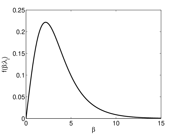
Clearly, the distribution vanishes at high and low temperatures when . For this quantum mechanical example, the low temperature limit of the energy is a finite constant. As a consequence, no extra constraint () is necessary to obtain a physical relevant distribution. The distribution is plotted in Fig. 1 for the example and .
VI Superstatistical classical ideal gas
As a second example we study a 3-dimensional classical ideal gas. The gas consists of particles with mass and is enclosed in a box with a volume equal to unity. The partition function and the energy of the ideal gas are
| and | (22) |
Inserting these formulas into the expression for the distribution (III) results in
| (23) |
The special case and was already studied in [35]. As mentioned before, in that case the distribution (23) is not normalizable and one has to restrict the values of to a finite range. In [37] the author noticed that an inverse gamma distribution is obtained for the choice , and .
Let us now comment on physically reasonable choices of the function . On physical grounds, in the various experimental applications of the superstatistics concept so far [26, 33, 13, 19, 34, 30], essentially three relevant distributions were observed for examples described by the superstatistical classical ideal gas: The gamma distribution, the inverse gamma distribution and the lognormal distribution. Some theoretical reasoning can be given [2] why this is so and why the above three distributions span up three relevant universality classes. It is now interesting to see that our generalized maximum entropy principle, in contrast to previous theoretical work, contains all these physically relevant cases. Depending on the choice of the function and the values of the Langrange multipliers one can extract the three relevant universal distributions out off expression (23). For convenience, we put . The gamma distribution is obtained for , and :
| (24) |
The inverse gamma distribution is obtained for , and :
| (25) |
The lognormal distribution is obtained for and :
| (26) | |||||
| (27) |
with
| (28) |
Unlike the quantum mechanical case, for classical complex systems usually is needed to make expectations formed with converge. This function is determined by additional information that one has on the complex system under consideration (an example will be treated in the next section).
Unlike the quantum mechanical case, for the classical ideal gas one has to be careful with a range of that goes from to . For this example the limiting behavior of the energy and the entropy at low temperatures is
| and | (29) |
The limit of the energy is acceptable from a thermodynamical point of view, the limit of the entropy is not. Clearly, the problem arises from the fact that the classical treatment of an ideal gas in the low-temperature limit does not make sense, one certainly has to take quantum corrections into account. However, when is vanishing in this limit, the contribution of the quantum region to the average values of the observables will be negligible. Notice that the three aforementioned distributions (24), (25), (27) all have a single peak at a well defined temperature. So as long as this single peak is situated in the classical region one can use classical models in the context of superstatistics although one has to be careful in evaluating the low temperature behavior of itself.
VII Turbulent Taylor-Couette flow

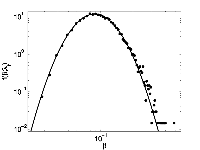

As a final example we now apply our methods to a complex system that is not analytically solvable anymore: Turbulent Taylor-Couette flow. Ideally, for a superstatistical statistical mechanics description of this system, one would measure the set of all positions and velocities of a large number of test particles in the flow. This is not possible and hence, as in previous papers [2], we restrict ourselves to the information that one can get out of a scalar time series, a single measured velocity component as a function of time . We use data from an experiment performed by Lewis and Swinney [40]. The stationary probability distribution of the velocity difference at a given scale is well-known to exhibit non-Gaussian behavior, see Fig. 2 for an example.
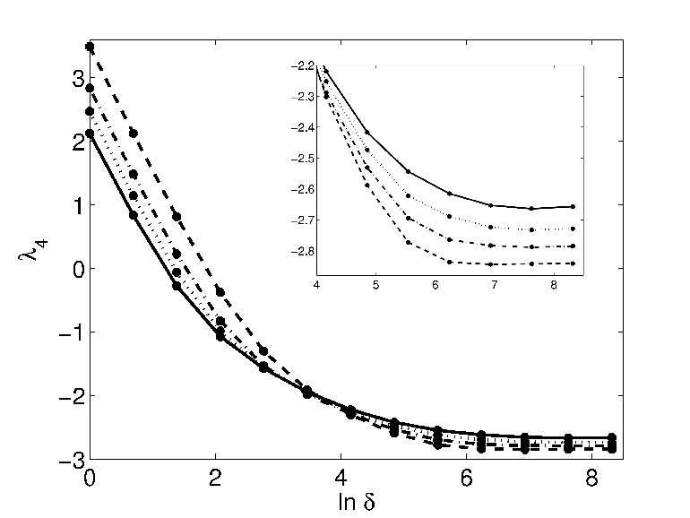
It has been previously shown that superstatistical techniques can be successfully used to model the statistics of turbulent velocity fluctuations [20, 25, 2, 26]. For a measured time series , the parameter simply corresponds to a local inverse variance of the measured signal, and the ‘cells’ of the superstatistics approach correspond to time slices of a suitable length where this variance is measured. The turbulent velocities are well approximated by the model of a classical ideal superstatistical gas, meaning that for certain time intervals the signal is Gaussian with a given variance, then it changes to another Gaussian with a different variance, and so on. The validity of the above approximation and the necessary time scale separation has been checked in a previous paper [2]. In that paper also a general method was introduced how to to extract the relevant time slicing (the superstatistical cell size) and how to extract the distributions from the signal. We do not describe this here in detail, but refer to the paper [2]. Using these techniques, we determined the distribution from the measured time series, using the experimental data of Swinney et al. for various scales and Reynolds numbers Re. In all cases, a lognormal distribution turns out to be a reasonable fit for the experimentally observed distribution , see Fig. 3 for an example. However, the parameters of this lognormal distribution depend on and Re in a nontrivial way. Our results are summarized in Fig. 4.
The relevance of lognormal distributions is to be expected due to the multiplicative random processes underlying the fluctuating energy dissipation in turbulent flows. In other words, the cascade picture of turbulence suggests that the constraint in the generalized maximum entropy principle should be of the form , leading to lognormal distributions. More surprising is the fact that our data analysis indicates that there is a distinguished scale , or , where the obtained fitting parameters are independent of Reynolds number. For , increases with increasing Reynolds number, whereas for it decreases. shows the opposite behavior, it decreases with Re for and increases for .
One may check the quality of the superstatistical model approximation by numerically evaluating the distribution [2]
| (30) |
and comparing it with the measured stationary distribution . Here is a lognormal distribution with parameters as given in Fig. 4. The solid line in Fig. 2 shows this curve (30) for the example . Clearly, there is an excellent agreement between the experimentally measured distribution and the superstatistical approximation (30).
Our turbulence example illustrates that the Lagrange multipliers in the generalized entropy maximization principle, and , do have physical meaning. Under different conditions, in our case fixed by the scale under consideration as well as the Reynolds number of the flow, these intensive parameters have different values (see Fig. 4). In fact, one could go as far as regarding the results in Fig. 4 to describe a kind of ’equation of state’ of the turbulent Taylor-Couette flow, providing the dependence of the intensive parameters and on given parameters of the flow pattern, such as scale and Re. All this illustrates that the generalized maximum entropy principles developed in this paper are not only a mathematical exercise, but of true physical relevance for a variety of classes of complex systems, when only a certain limited amount of information on the system is available.
VIII Conclusion
In this paper we developed a maximum entropy principle for superstatistical systems of various kinds. This principle allows for the determination of the superstatistical distribution of the fluctuating intensive parameter , given some prior information on the complex system under consideration. Our formalism further develops previous work of Abe et al., Crooks, and Naudts, and contains physically relevant superstatistical universality classes, such as lognormal superstatistics, gamma superstatistics and inverse gamma superstatistics, as special cases. We dealt with 3 important physical examples, the superstatistical quantum harmonic oscillator, the superstatistical classical ideal gas and time series as generated by a turbulent Taylor-Couette flow. For the quantum case, a new single-peaked distribution as displayed in Fig. 1 arises quite naturally out of our maximum entropy approach, whose physical relevance can be checked in future experiments. For classical systems, other types of distributions are relevant, such as the lognormal distribution for turbulent flows, as displayed in Fig. 3. Our approach is a further step to arrive at a generalized statistical formalism relevant for large classes of complex systems with time scale separation.
References
- [1] C. Beck and E.G.D. Cohen, Superstatistics, Physica A 322, 267 (2003)
- [2] C. Beck, E.G.D. Cohen, and H.L. Swinney, From time series to superstatistics, Phs. Rev. E 72, 026304 (2005)
- [3] C. Beck and E.G.D. Cohen, Superstatistical generalization of the work fluctuation theorem, Physica A 344, 393 (2004)
- [4] H. Touchette and C. Beck, Asymptotics of Superstatistics, Phys. Rev. E 71, 016131 (2005)
- [5] C. Tsallis and A.M.C. Souza, Constructing a statistical mechanics for Beck-Cohen superstatistics, Phys. Rev. E 67, 026106 (2003)
- [6] A.K. Rajagopal, Superstatistics – a quantum generalization, cond-mat/0608679
- [7] P. Jizba, H. Kleinert, Superpositions of probability distributions, arXiv:0802.0695
- [8] C. Vignat, A. Plastino and A.R. Plastino, Superstatistics based on the microcanonical ensemble, cond-mat/0505580
- [9] P.-H. Chavanis, Coarse grained distributions and superstatistics, Physica A 359, 177 (2006)
- [10] G. Wilk and Z. Wlodarczyk, Interpretation of the nonextensivity parameter in some applications of Tsallis statistics and Levy distributions, Phys. Rev. Lett. 84, 2770 (2000)
- [11] C. Beck, Dynamical foundations of nonextensive statistical mechanics, Phys. Rev. Lett. 87, 180601 (2001)
- [12] F. Sattin, Superstatistics from a different viewpoint, Physica A 338, 437 (2004)
- [13] K. E. Daniels, C. Beck, and E. Bodenschatz, Generalized statistical mechanics and defect turbulence, Physica D 193, 208 (2004)
- [14] C. Beck, Generalized statistical mechanics of cosmic rays, Physica A 331, 173 (2004)
- [15] M. Baiesi, M. Paczuski and A.L. Stella, Intensity thresholds and the statistics of temporal occurence of solar flares, Phys. Rev. Lett. 96, 051103 (2006)
- [16] Y. Ohtaki and H.H. Hasegawa, Superstatistics in econophysics, cond-mat/0312568
- [17] A.Y. Abul-Magd, Superstatistics in random matrix theory, Physica A 361, 41 (2006)
- [18] S. Rizzo and A. Rapisarda, Environmental atmospheric turbulence at Florence airport, Proceedings of the 8th Experimental Chaos Conference, Florence, AIP Conf. Proc. 742, 176 (2004) (cond-mat/0406684)
- [19] A. Porporato, G. Vico, and P.A. Fay, Superstatistics in hydro-climatic fluctuations and interannual ecosystem productivity, Geophys. Res. Lett. 33, L15402 (2006)
- [20] A. Reynolds, Superstatistical mechanics of tracer-particle motions in turbulence, Phys. Rev. Lett. 91, 084503 (2003)
- [21] N.G. van Kampen, Stochastic processes in physics and chemistry, North-Holland, London (1982)
- [22] S.L. Heston, A closed-form solution for options with stochastic volatility with applications to bond and currency options, Rev. Fin. Studies 6, 327 (1993)
- [23] R. Kubo, M. Toda and N. Hashitsume, Statistical Physics II: Nonequilibrium statistical mechanics, Springer, New York (1995)
- [24] W. Feller, An introduction to probability theory and its applications, Vol. II, John Wiley, London (1966)
- [25] C. Beck, Lagrangian acceleration statistics in turbulent flows, Europhys. Lett. 64, 151 (2003)
- [26] C. Beck, Statistics of 3-dimensional Lagrangian turbulence, Phys. Rev. Lett. 98, 064502 (2007)
- [27] M. Ausloos and K. Ivanova, Dynamical model and nonextensive statistical mechanics of a market index on large time windows, Phys. Rev. E 68, 046122 (2003)
- [28] J.-P. Bouchard and M. Potters, Theory of Financial Risk and Derivative Pricing, Cambridge University Press, Cambridge (2003)
- [29] H. Aoyama et al., Productivity dispersion: Facts, theory, and implications, arXiv:0805.2792
- [30] A.Y. Abul-Magd, B. Dietz, T. Friedrich, A. Richer, Spectral fluctuations of billiards with mixed dynamics: from time series to superstatistics, Phys. Rev. E 77, 046202 (2008)
- [31] S. Abe and S. Thurner, Complex networks arising from fluctuating random graphs, Phys. Rev. E 72, 036102 (2005)
- [32] Sílvio M. Duarte Queirós, On Superstatistical Multiplicative-Noise Processes, Braz. J. Phys. 38, 203 (2008)
- [33] K. Briggs, C. Beck, Modelling train dealys with q-exponential functions, Physica A 378, 498 (2007)
- [34] L. Leon Chen, C. Beck, A superstatistical model of metastasis and cancer survival, Physica A 387, 3162 (2008)
- [35] S. Abe, C. Beck and G. D. Cohen, Superstatistics, thermodynamics, and fluctuations, Phys. Rev. E 76, 031102 (2007)
- [36] G. E. Crooks, Beyond Boltzmann-Gibbs statistics: Maximum entropy hyperensembles out of equilibrium, Phys. Rev. E 75, 041119 (2007)
- [37] J. Naudts, Generalised thermostatistics using hyperensembles, AIP Conference Proceedings 84, 965 (2007)
- [38] R. D. Rosenkrantz, E.T. Jaynes: papers on probability, statistics and statistical physics, Kluwer (1989)
- [39] C. Tsallis, Possible generalization of Boltzmann-Gibbs statistics, J. Stat. Phys. 52, 479 (1988)
- [40] G. S. Lewis and H. L. Swinney, Velocity structure functions, scaling, and transitions in high-Reynolds-number Couette-Taylor flow, Phys. Rev. E 59, 5457 (1999)