CQUeST-2008-0208
Geodesic Properties and Orbits in 5-dimensional Hypercylindrical Spacetime
11 1 email:rasenis@sogang.ac.kr 22 2 email:bhl@sogang.ac.kr and 33 3 email:warrior@sogang.ac.kr
†Department of Physics, Sogang University, Seoul 121-742,
Korea
¶Center for Quantum Spacetime, Sogang University, Seoul 121-742,
Korea
§Research Institute for Basic Science, Sogang University, Seoul 121-742,
Korea
Abstract
We investigate the geodesic motions of a massive particle
and light ray in the hyperplane orthogonal to the symmetry axis in
the 5-dimensional hypercylindrical spacetime. The class of
the solutions depends on one constant which is the ratio of
string mass density and tension. There exist unstable orbits in
null geodesic only in some range of . The innermost stable
circular orbits in timelike geodesic also exist only in a certain
range of the parameter . The capture cross section
and the deflection angle of light ray are also computed.
PACS numbers : 04.50.+h, 04.70.-s, 04.90.+e
1 Introduction
In the study of the hierarchy problem, the extra dimension has done important roles [1]. The extra dimension does not have to be compactified 5th dimension. Our universe can be viewed as a 4-dimensional brane world embedded in the 5-dimensional spacetime. From the analysis of brane world with large extra dimension, interesting 5-dimensional black object solutions have been presented [2]. The simplest model may be the Schwarzschild black string, whose instability was also examined [3].
General class of solutions including the Schwarzschild black string were discovered by Kramer [4], Gross and Perry [5], Davidson and Owen [6], and Lee [7]. This class of the 5-dimensional solutions depends on an arbitrary constant . This solution has a naked singularity, and we need to consider the physical possibility of the metric. Virbhadra and Ellis [8] classified naked singularities into weakly and strongly naked ones. There exist parameter range in which singularity is weakly and strongly naked one in our analysis. According to their classification, the singularity of the metric studied in the present work and in the Refs. [7, 9, 10, 11] corresponds to a weakly naked one. Virbhadra and Ellis studied the possibility for observing the naked singularity based on the gravitational lensing effect, pointing out that the cosmic censorship hypothesis of Penrose has not been completely proven. It was also shown by K. S. Virbhadra and C. R. Keeton in Ref. [12] that this observational method may play the role of more efficient cosmic telescopes, if singularities exist in nature. Virbhadra and Ellis also pointed out that the observational properties of the weakly naked singularity as in the metric in our paper will be shown to be similar to those of the Schwarzschild black hole. With all these and in relation to the observation of the singularity in the future, it is worthwhile to investigate the properties of our metric, as has been done by authors in Refs. [7, 9, 10, 11].
In Ref. [7], this constant is interpreted as the ratio of string mass density and tension. This solution corresponds to the Schwarzschild black string for . In addition, the solution becomes the Kaluza-Klein bubble [13] for . Extension of the string to the p-brane solutions with mass and tension were constructed in Ref. [14]. In Ref. [9], the authors studied some geometrical properties such as the location of curvature singularity, proper length of 5 dimension, and casual structure based on the radial null geodesics. The hypercylindrical solution is asymptotically flat in both and [10] .
The stationary vacuum cylindrical solution with momentum in translational direction were investigated [15]. In this solution it was shown that the compactification along -direction breaks the Lorentz symmetry, which makes the frame dragging effect into the physical observable [16]. It was shown that there are vacuum stationary black string solutions, other than the Schwarzschild black string solution in 5-dimensional spacetime [17]. These can lead to a new class of solutions, and its properties were studied in Ref. [18, 19, 20]. The formation of five-dimensional solutions [7] from the gravitational collapse and its numerical works are presented in Ref. [11]. A black string from - and -strings in a system are studied in Ref. [21]. These objects may play the role of gravitational lenses with modifying the properties [22, 12].
Due to the complexity of this solution, much of the properties are not yet known. In this paper we study the geodesics and the orbits according to .
The organization of this paper is as follows. In Sec. 2, we briefly review the hypercylindrical solutions. We summarize the physical meaning of the constant , the condition for event horizon, the Schwarzschild black string, and the Kaluza-Klein bubble. In Sec. 3, the main results are calculated [23]. We derive the geodesics for null and timelike from Lagrangian, and get conserved quantities using Killing vectors. The range of giving rise to unstable circular orbit is obtained by analyzing the effective potential. The diffraction angle of bending light is also studied. Timelike geodesics are analyzed by analytic and numerical methods. In addition, some properties of orbits are numerically computed. In Sec. 4, we summarize the results with discussion.
2 Brief Review on the hypercylindrical Solutions
A general class of the hypercylindrical solutions with an arbitrary constant is found and explained in Ref. [7]. The tension of the string and its mass density are related by
| (1) |
In Ref. [24], the author studied the positive tension due to pure gravitational contribution. In addition, if one demands that the strong energy condition be satisfied, there exists the upper bound, [9]. We will consider the general case including the negative tension.
The metric ansatz for hypercylindrical solutions is written as
| (2) |
The components of the metric satisfying the asymptotical flatness are [7]
where and .
The metric has the transverse spherically symmetric static property. We will consider the range of , .
In the above solutions, is an arbitrary constant not depending on coordinate variables. The causal structure of this spacetime is described in Ref. [9] by analyzing the radial null geodesics. In that paper, they show that an event horizon exists only for the case , which correspond to the Schwarzschild black string. For other values of , the metric becomes singular at , as pointed out in Ref. [14]. This singularity corresponds to a weakly naked one in Ref. [8].
As some special cases, we consider four cases of , which give different types of solutions. For the constant , the string tension vanishes, and the metric becomes
| (3) | |||||
where .
For value of , the metric becomes that of the Schwarzschild black string given by
| (4) |
where .
For , the metric is given as follows
| (5) |
where . Note that the metric functions and are the same.
3 Geodesic Properties and Orbits
One define Lagrangian as
| (7) |
where denotes the differentiation with respect to the affine parameter . For timelike, null and spacelike case, is equal to -1, 0 and 1, respectively.
The geodesic equation is given by the Euler-Lagrange equation
| (8) |
The metric is invariant under translations , , and . Accordingly, the conjugate momenta , , and are conserved. Using the Killing vectors , , and from the metric symmetries of , , and , respectively, the conserved quantities are expressed as
From Lagrangian, we get the following equations
| (9) |
where the conversed quantities , , and are the energy, angular momentum, and linear momentum, respectively. In general, this kind of metric has additional conserved quantities such as . The setting on the equatorial plane, is related to the remaining two Killing vectors, which lead to the conservation of the direction of angular momentum. Thus, in this setting, conserved quantities are three: , , and , which are integration constants. In this paper, we can take without loss of generality, and we investigate the case of no 5-dimensional momentum to see 4-dimensional cases.
To obtain the orbits in this spacetime, we construct the effective potential. The potential can be obtained from Lagrangian in Eq. (7). Using Eq. (9), the Lagrangian in Eq. (7) becomes
| (10) |
This can be rewritten as
| (11) |
where and This equation governs the geodesics in the given spacetime. In the analysis of the geodesic motions, we can directly read off the behaviors of the motions from the shape of the effective potential. Stable circular orbits are possible if the potential has a minimum point. On the other hand, unstable circular orbits are possible if the potential has a maximum point. For example, there are stable circular orbits in the case of timelike geodesics in the Schwarzschild black hole spacetime, while there are unstable circular orbits in the case of null geodesics in the spacetime [25].


The effective mass is written
| (12) | |||||
Objects which is located in have different mass called effective mass as the location is approached to . It makes that the object is looked like having mass even if light. The effective mass is categorized two types by its behavior in the vicinity of . The effective mass depends on the location , approaching asymptotically 1 in any choice of . The behavior of effective mass is divided by ’s exponent. The exponent with the base change sign at (Fig. 1). The effective mass at becomes zero in , and infinite in (Fig. 2).
3.1 The Null Geodesics
The Lagrangian for null geodesics becomes
| (13) |
The geodesic equation of for light ray is given by
| (14) |
From Eq. (13)
| (15) |
After inserting this result into the geodesic equation Eq. (14), we get
| (16) |
From Eq. (9) and Eq. (15), we get the relations between coordinate components as follows


We consider the orbits of null geodesics satisfying and . The effective potential, , of the 4-dimensional null Lagrangian becomes
| (17) | |||||
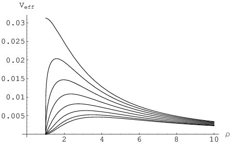
The effective potentials according to are shown in Fig. 4. The maximum point in the potential indicate the location of the unstable circular orbit. The photon spheres corresponds to the location of maximum points in the effective potential for each values of the constant . The surface of photon spheres contain the region of . This type of singularity is called a weakly naked singularity. Note that can not be smaller than .
The angular momentum appears as scaling factor of this potential, this is from the fact that the potential expresses the light motion. The constant is the only variable determining the shape of the potential. To get unstable circular orbits in the potential, we calculate the extrema of the potential. The location is given by
| (18) |
where this is the only possible circular orbit.
From the reality of , the range of is given by
| (19) |
The location of the unstable circular orbit is dependent on the constant . The behavior of the location can be read off directly from the Fig. 4. Note that there are no stable circular photon orbits in this spacetime for like the case of the Schwarzschild black hole. There exist parameter range in which singularity is weakly naked one, , and strongly naked one, or , in our analysis.
The light ray with impact parameter smaller than specific value is captured by the strong gravitational field. Using this parameter, the capture cross section can be calculated. From trajectories of and , 4-dimensional Lagrangian can be written as
| (20) |
where is impact parameter. From above equation, the potential impact parameter can be defined as
| (21) |
This potential impact parameter is interpreted as the condition restricting the evolution of null geodesic [25]
Thus, the minimum value of is the critical impact parameter, . For example, the value of critical is in the Schwarzschild case. Since the shape of is relative to the inverse . The minimum point of is the same as maximum point of . To get the minimum point, the partial derivative is needed
| (22) |
Similar analogy can be done. The same result can be obtained by . The critical value of impact parameter is . Explicitly, is redefined to . For , the is written as
| (23) | |||||
For example, the incident light ray whose impact parameter is smaller than is captured by the gravity of the black hole. The area exists for . The area is the capture cross section [26], , is given by
| (24) |
The graph is plotted in Fig. 5.

We now calculate the bending of light in the gravitational field. To see this bending, we get the trajectory of light rays, using the symmetry of the spacetime.

The closest distance is the minimum point of the function, . The equation
| (25) |
can have two solutions. One of them is the point where vanishes. In the case, the trajectory of light always touch the singular point, we will not consider this solution. The other solution comes from
| (26) |
The solutions of this equation exist in specific range of constant and can be found by numerical calculation. To get the range, we observe is asymptotically(large ) proportional to . With the behavior of asymptotic region, the term must be zero at the point to cover all region of positive values. Thus, the range of constant which gives the region is


| a=-10 | a=-5 | a=-3 | a=4 | a=5 | a=10 | |
| L=1 | 1.4472 | 1.2999 | 1.14769 | 1.14769 | 1.2365 | 1.42959 |
| L=2 | 2.15922 | 1.91702 | 1.61759 | 1.61759 | 1.80134 | 2.13164 |
| L=3 | 3.01022 | 2.72839 | 2.36845 | 2.36845 | 2.59145 | 2.97837 |
The angle is expressed by
| (27) |
This equation is redefined to make dimensionless as
From now on, we drop tilde for simplicity. The case of light is set to . The value of is relatived to by
| (28) |
Using above table and Eq. (28), the deflection angle is computed for some values of or in table 2.
| a=-10 | a=-5 | a=-3 | a=4 | a=5 | a=10 | |
| L=1 | -1.12253 | -1.22649 | -1.22649 | -1.14726 | -1.10551 | |
| L=2 | -2.17775 | -0.24806 | -0.0552344 | -0.055234 | -0.375315 | |
| L=3 | 0.030895 | 0.295974 | 0.295974 | 0.124414 | -0.118769 |
| a=-1 | a=0 | a=0.5 | a=2 | ||||||||
|---|---|---|---|---|---|---|---|---|---|---|---|
| L | L | L | L | ||||||||
| 4.12 | 1.41157 | 4.32406 | 9.8 | 5.15716 | 2.03338 | 12.3 | 7.13644 | 1.57997 | 4.12 | 1.41157 | 4.32406 |
| 7 | 4.79129 | 0.903441 | 12 | 7.8105 | 1.12041 | 16 | 11.3127 | 0.847878 | 7 | 4.79129 | 0.903441 |
3.2 The Timelike Geodesics
For the timelike geodesic, . Using Eq. (8) and Eq. (9) the equation becomes
| (29) |
where the prime denotes the differentiation with respect to .
From Eq. (7) we get
| (30) |
Inserting this result into the geodesic equation of , we obtain
| (31) |
We get the relations between coordinate components as follows
The timelike case allows stable circular orbits in some range of the constant . The effective potential for timelike geodesics is
| (32) | |||||
First, we investigate radial motion of the effective potential L=0 in Eq. (3.2) The behavior of the effective potential is shown in Fig. 8.


The potential is different from the null case due to the second term for not . To get the stable circular orbits, the asymptotic behaviors of and must be analyzed. In asymptotic region, , each term becomes as follows
| (33) |
As we can see in Eq. (33), the asymptotic values are not affected by the constant . So the key conditions may be the behaviors of in the vicinity of . At the point of , a convergent condition of is . The calculation shows that at in .

For the existence of closed orbit, we require be divergent at , which gives the exponent being negative. this gives or . We also want becomes zero at which gives . Thus, overlapping range for these conditions is . In this region, the potential always has its minimum point, and the matter can be moved following stable orbits. One of the circular orbit cases in the timelike potential can be made from combination of and as shown in Fig. 9. Finding the condition of which exists the combination at the same time is the key point in its analysis. Note that any angular momentum value is allowed.


In the range of , the orbit can exist only for as in the Schwarzschild spacetime case if . The orbit at is called the marginal stable circular orbit or the innermost stable circular orbit. Some exaples are shwon in Fig. 10.
| -1 | -0.5 | 0 | 0.5 | 1 | 1.5 | |
|---|---|---|---|---|---|---|
| 2.9 | 4.8 | 6.4 | 7 | 5.2 | 3 | |
| 1.56673 | 4.59308 | 7.54371 | 8.38068 | 9.07818 | 5.48575 |
From the Fig. 10, we see that there are finite potential barrier due to the angular momentum for the cases of , and . On the other hand, the potential barrier preventing a particle reaching deep inside appears appeared for the case of .
For some specific values of constant , the effect of angular momentum and marginal orbit is shown at Fig. 10, and this table 4 shows marginal orbit’s radius and values of angular momentum. As can be seen in the table 4, the angular momentum which makes the marginal orbit becomes largest for while the radius of marginal orbits becomes the largest approximately .
4 Summary and Discussions
In this paper, we have studied the geodesic motions and the orbits of both a massive particle and light ray. The geometry of the hypercylindrical solution is dependent on single constant , a ratio of tension and mass density. This geometry becomes that of the Schwarzschild black string for , and the static Kaluza-Klein bubble for . There exist five conserved quantities corresponding to translation symmetry of time, angle, 5th dimension coordinate, and two quantities which give equatorial plane . The quantities are E, L, and W related to time, angle, and 5th coordinate. The geodesic equations for null and timelike case is given by Euler-Lagrangian equations. To get orbits, we obtained the effective potential from the Lagrangian. We get effective mass from the equation. Effective mass is asymptotically flat, but it becomes zero at in , and infinite in . The light can move around a unstable circular orbit in . The radial range of the unstable circular orbit is related to area of light capture. The capture cross section is formed in , and the largest area case is Schwarzschild black string. The property of the metric at in our paper has already been studied by the authors in Ref. [14]. The curvature of the metric was shown to be singular at the point except for and in the range of . The geometry described by the hypercylindrical solution affects null trajectories. The deflection angle is obtained to show this effect. We get two range of constant a where null trajectories behave differently. The deflection angles are similar to black hole case in and behave differently in or . There exist parameter range in which singularity is weakly naked one, , and strongly naked one, or , in our analysis. We calculate the timelike geodesic equations and the range of the constant which gives stable circular orbits in . One of the characteristics of the timelike case is that there exist a marginal stable circular orbit in . The angular momentum and radius of this marginal orbit is numerically obtained, and the shapes of the effective potentials are similar to Schwarzschild black string in .
According to Virbhadra and Ellis, the singularity of the metric studied in the present work and in the Refs. [7, 9, 10, 11] corresponds to a weakly naked one. In other wards, Fig. 4 in our paper indicates that there exist photon spheres [27] from . The observational properties of our spacetime is indistinguishable from the Schwarzschild black hole [8]. They may play the role of more efficient cosmic telescopes, if these singularities exist in nature [12]. The authors in Ref. [12] modeled the massive dark objects at galactic centers as these singularities including a Schwarzschild black hole.
With all these and in relation to the observation of the singularity in the future, it is worthwhile to investigate for the properties of the hypercylindrical spacetime. For instant, the scattering of waves is one of them. Based on the information about the reflected wave, the reflecting rate and scattering cross section can be calculated. This work is in progress.
Acknowledgments
We would like to thank Gungwon Kang, Hyeong-Chan Kim, Chanyong Park and Myungseok Yoon for valuable discussions and kind comments. We would like to thank Jungjai Lee, Inyong Cho, and Chan-Gyung Park for their kind comments at the Workshop on Numerical Relativity, June, 2008. This work was supported by the Science Research Center Program of the Korea Science and Engineering Foundation through the Center for Quantum Spacetime (CQUeST) of Sogang University with grant number R11 - 2005- 021. WL was supported by the Korea Research Foundation Grant funded by the Korean Government(MOEHRD)(KRF-2007-355-C00014).
References
- [1] N. Arkani-Hamed, S. Dimopoulos, and G. R. Dvali, Phys. Letts. B 429, 263 (1998); I. Antoniadis, N. Arkani-Hamed, S. Dimopoulos, and G. R. Dvali, Phys. Letts. B 436, 257 (1998); L. Randall and R. Sundrum, Phys. Rev. Lett. 83, 3370 (1999); 83, 4690 (1999); H. B. Kim and H. D. Kim, Phys. Rev. D 61, 064003 (2000); J. Garriga and T. Tanaka, Phys. Rev. Lett. 84, 2778 (2000); C. Kokorelis, Nucl. Phys. B 677, 115 (2004).
- [2] A. Chamblin, S. W. Hawking, and H. S. Reall, Phys. Rev. D 61, 065007 (2000); A. Chamblin, H. S. Reall, H.a. Shinkai, and T. Shiromizu Phys. Rev. D 63, 064015 (2001); W. T. Kim, J. J. Oh, M. K. Oh, and M. S. Yoon, J. Korean Phys. Soc. 42, 13 (2003); C. H. Coimbra-Araujo and P. S. Letelier, Phys. Rev. D 76, 043522 (2007).
- [3] R. Gregory and R. Laflamme, Phys. Rev. D 37, 305 (1988); Nucl. Phys. B 428, 399 (1994); R. Gregory, Class. Quant. Grav. 17, L125 (2000); G. T. Horowitz and K. Maeda, Phys. Rev. Lett. 87, 131301 (2001); T. Hirayama and G. Kang, Phys. Rev. D 64, 064010 (2001); T. Wiseman, Class. Quant. Grav. 20, 1177 (2003); G. Kang and J. Lee, J. High Energy Phys. 03 (2004) 039; M.-I. Park, Class. Quant. Grav. 22, 2607 (2005); T. Harmark, V. Niarchos, and N. A. Obers, Class. Quant. Grav. 24, R1 (2007).
- [4] D. Kramer, Acta Phys. Polon. B 2, 807 (1970).
- [5] D. J. Gross and M. J. Perry, Nucl. Phys. B 226, 29 (1983).
- [6] A. Davidson and D. A. Owen, Phys. Letts. B 155, 247 (1985).
- [7] C. H. Lee, Phys. Rev. D74, 104016 (2006).
- [8] K. S. Virbhadra and G. F. L. Eliis, Phys. Rev. D 65, 103004 (2002).
- [9] I. Cho, G. Kang, S. P. Kim, and C. H. Lee, [arXiv:0709.1021]
- [10] G. Kang, I. Cho, S. P. Kim, and C. H. Lee, KISTI-2007 (in preparation).
- [11] S. Hyun, J. Jeong, W. Kim and J. J. Oh, Class. Quant. Grav. 24, 3465 (2007).
- [12] K. S. Virbhadra and C. R. Keeton, Phys. Rev. D 77, 124014 (2008).
- [13] E. Witten, Nucl. Phys. B 195, 481 (1982); H. Elvang, T. Harmark, and N. A. Obers, J. High Energy Phys. 01 (2005) 003.
- [14] J. Lee, G. Kang, and H. C. Kim, [arXiv:0801.0482].
- [15] J. Lee and H. C. Kim, Mod. Phys. Lett. A 22, 2439 (2007).
- [16] J. Lee and H. C. Kim, Mod. Phys. Lett. A 23, 305 (2008).
- [17] H. C. Kim and J. Lee, Phys. Rev. D 77, 024012 (2008).
- [18] J. L. Hovdebo and R. C. Myers, Phys. Rev. D 73, 084013 (2006).
- [19] A. Chodos and S. Detweiler, General Rel. and Grav. 14, 879, (1982).
- [20] G. Clement, General Rel. and Grav. 16, 131, (1984); General Rel. and Grav. 16, 491, (1984).
- [21] T. Kim, Y. Kim, B. Kyae, and J. Lee, Phys. Rev. D 77, 065027 (2008).
- [22] S. Resfsdal, Mon. Not. R. Astron. Soc. 128, 295 (1964); R. D. Blandford and R. Narayan, Ann. Rev. Astron. Astrophys. 30, 311 (1992); K. S. Virbhadra and G. F. R. Ellis, Phys. Rev. D 62, 084003 (2000); R. Whisker, Phys. Rev. D 71, 064004 (2005); M. V. Sazhin et al., Mon. Not. R. Astron. Soc. 376, 1731 (2007); K. S. Virbhadra, arXiv:0810.2109.
- [23] B. Gwak, M. S. thesis, Sogang University, 2007 (unpublished).
- [24] J. Traschen, Class. Quant. Grav. 21, 1343 (2004).
- [25] C. W. Misner, K. S. Thorne, and J. A. Wheeler, Gravitation (Freeman, San Francisco, 1973).
- [26] D. Raine and E. Thomas, Black Holes : An Introduction (Imperial College Press, London, 2005).
- [27] C.-M. Claudel, K. S. Virbhadra, and G. F. R. Ellis, J. Math. Phys. 42, 818 (2001).