Ferromagnetic resonance force spectroscopy of individual sub-micron size samples
Abstract
We review how a magnetic resonance force microscope (MRFM) can be applied to perform ferromagnetic resonance (FMR) spectroscopy of individual sub-micron size samples. We restrict our attention to a thorough study of the spin-wave eigen-modes excited in permalloy (Py) disks patterned out of the same 43.3 nm thin film. The disks have a diameter of either or m and are quasi-saturated by a perpendicularly applied magnetic field. It is shown that quantitative spectroscopic information can be extracted from the MRFM measurements. In particular, the data are extensively compared with complementary approximate models of the dynamical susceptibility: i) a 2D analytical model, which assumes an homogeneous magnetization dynamics along the thickness and ii) a full 3D micromagnetic simulation, which assumes an homogeneous magnetization dynamics below a characteristic length scale and which approximates the cylindrical sample volume by a discretized representation with regular cubic mesh of lateral size nm. In our analysis, the distortions due to a breaking of the axial symmetry are taken into account, both models incorporating the possibility of a small misalignment between the applied field and the normal of the disks.
I Introduction
Development of innovative tools capable of measuring the local magnetization dynamics inside a ferromagnetic nano-structure is an objective of primary importance. New technology fields related to magnetic materials, like spintronics, depend on one’s ability to analyze and predict the out-of-equilibrium state of in nanoscale hybrid structures. In this respect, models derived from microscopic principles are often limited because of the numerous degrees of freedom strongly coupled to the magnetization. Hence, phenomenological approaches are often used, and require a constant comparison with experiments.
Several original techniques are being pursued to measure the dynamics of on small length scales. Among them, X-ray magnetic circular dichroism (XMCD) transmission microscopy [1, 2], XMCD photoelectron microscopy (PEEM) [3], microfocus Brillouin light scattering (BLS) [4], time-resolved scanning Kerr microscopy (TRSKM) [5, 6, 7], spin-torque driven ferromagnetic resonance (ST-FMR) [8, 9, 10] and magnetic resonance force microscopy (MRFM) applied to ferromagnetic resonance [11, 12, 13] are the most accomplished yet. This article focuses on the last one, called herein mechanical-FMR, since a mechanical setup is used for the detection of FMR, as shown in Fig.1. Here, we shall review the ability of mechanical-FMR to extract quantitative spectroscopic information in individual samples.
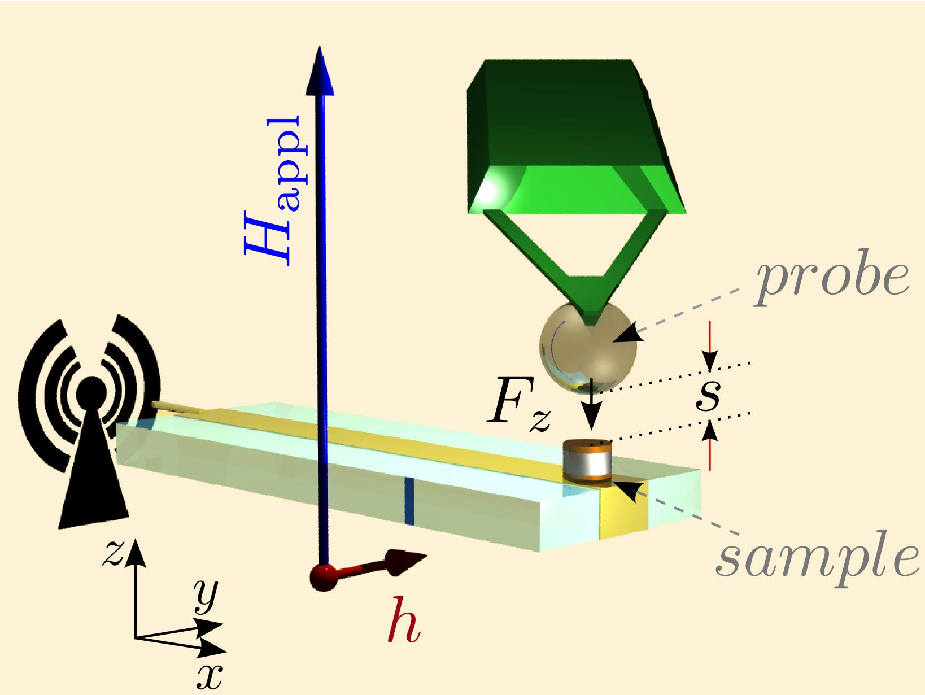
In FMR, the magnitude of the magnetization vector, , is a constant of the motion and equals the saturation magnetization at the lattice temperature. Thus the dynamics of is governed by the position- and time-dependent transverse fluctuations of the magnetization direction, the so-called spin-waves (SW) [14] , where is the longitudinal component of the magnetization, defined as the projection of the instantaneous vector along the local precession (or equilibrium) axis of unit vector . Because of the exchange interaction, these transverse fluctuations are a collective precession, and become more insightful once decomposed along the normal modes basis of the sample. Therefore the experimental identification of this SW basis is important. Its nature depends primarily on the symmetry of the equilibrium configuration of inside the sample [15]. In the case of a uniformly magnetized sample, the SW confinement is mostly governed by the shape of the sample. In thin films, the quantization of the lowest energy (or longest wavelength) modes develops along the finite thickness direction, whereas in nanostructures, it arises both from the thickness and lateral confinements.
Although, there are fundamental interests in studying the magnetization dynamics in the time domain (or free precession regime), the best spectral resolution is obtained by continuous wave spectrometers, which study the harmonic response (or forced oscillation regime). Conventional spectrometers excite and detect the SW eigen-modes of a ferromagnetic sample with the same microwave antenna. In a conventional-FMR experiment [16], the sample is placed in a region where a large homogeneous static magnetic field aligns the spins in a well-defined direction. On the emission side, a small microwave field , applied perpendicularly to the effective magnetic field (), will cant the magnetization away from its equilibrium axis if the resonance condition is met, i.e. if the photon energy () corresponds to the energy to excite one SW or magnon (). The symmetry of the excitation antenna sets the selection rules and the symmetry of the excited SW. On the reception side, the measured quantity in a conventional spectrometer is , the microwave energy absorbed inside the sample per unit of time. Technically, is obtained by monitoring the transmitted or reflected power to a microwave diode, whose dc voltage is proportional to the incident microwave power. In metallic samples, the absorbed power per unit of surface can be expressed as a function of , the complex surface impedance of the sample [17, 18], which itself depends on the complex electrical conductivity and magnetic susceptibility. For thin magnetic layers, it mainly reduces to the dissipative part of the microwave transverse magnetic susceptibility, as in insulators: , where the shorthand notation represents the time derivative.
The dependence of on either the applied magnetic field, , or the frequency of the excitation source, , reveals resonance peaks (bell-shaped curves). Their positions, amplitudes and line widths reflect the complete spectral information about the spin system. i) The position is a precise measurement of the effective magnetic field defined as the conjugate variable of the magnetization, , where is the free energy of the spin system. ii) The amplitude is related to the coupling (overlap integral) with both the excitation and the detection schemes. It thus gives a hint about the spatio-temporal profile of the mode. For instance, with a cavity (cavity-FMR) or a stripline antenna (stripline-FMR), the microwave field is uniform over the sample volume. As a result, it preferentially couples to the longest wavelength SW modes of the sample. iii) The frequency line width gives the decay rate of the excited SW (coherent with ) to the other degrees of freedom: the degenerate and thermal SW (incoherent with ) or the lattice (electrons and phonons). In Bloembergen and Wang’s notation [19], the line width is proportional to [20]. Experimentally, it is often easier to monitor the dependence of when is swept at fixed . In this case, it is crucial to repeat the measurement at several frequencies and to renormalize the field line width by the effective gyromagnetic ratio .
FMR spectroscopy is usually restricted to probe tiny deviations of the magnetization from its equilibrium. First, reaching large angles of precession requires a lot of microwave energy, especially in metallic samples and second, the interpretation of the high power regime requires a specific analysis since the equation of motion is non-linear [21]. The typical angles of precession found in FMR are less than . Although FMR is a sensitive technique, still the sensitivity of most conventional spectrometers is usually not sufficient to detect magnetization dynamics in individual sub-micron size samples. The crucial parameter here is the ratio between the volume of the sample and the volume of the detector: the so-called filling factor. With the recent development of MRFM, the sensitivity of magnetic resonance has been tremendously enhanced. Nanometer scale sizes come now within reach as Dan Rugar and colleagues at IBM Almaden recently showed with the detection of a single electron spin [22] and with a record 90 nm resolution on nuclear paramagnets, where only a few thousands of nuclear spins contribute to the signal [23]. The key to such performance comes from the size of the magnetic probe, which has a very strong coupling with the resonant volume, thus ensuring an almost optimized filling factor.
In this paper, we show how a mechanical-FMR setup can be used to perform FMR spectroscopy of sub-micron size samples. We present a thorough study of the SW eigen-modes in individual permalloy (Py) disks, whose FMR spectra are compared to a 2D approximate analytical model and to full 3D micromagnetic simulations of the dynamical susceptibility. The structure of the rest of the paper is the following. Section II presents the principles of the mechanical-FMR and gives an extensive analysis of the spectral deformations induced by the magnetic probe on the measured FMR spectra. In section III, the experimental results are presented. In section IV, we derive an approximate 2D analytical model and present the results of a 3D micromagnetic simulation. They are both used in section V to analyze the data. Section VI contains a summary of the results obtained.
II Mechanical-FMR
II.1 The experimental setup
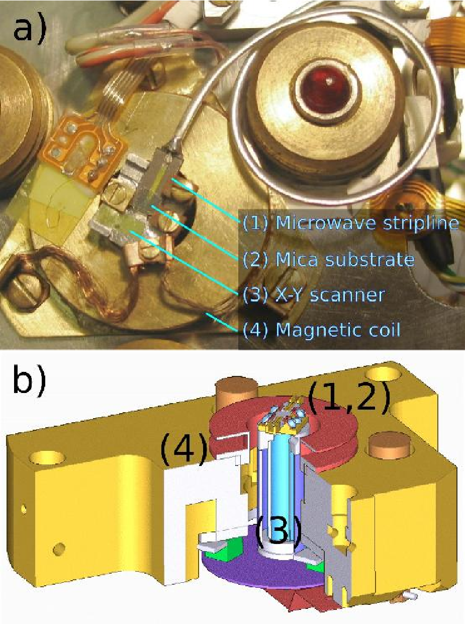
The concept of mechanical detection of the magnetic resonance was first applied to FMR by Phil Wigen and Chris Hammel in 1996 [11]. Fig.1 illustrates the mechanical-FMR setup, while Fig.2 presents its experimental realization for the present study.
II.1.1 Excitation part
The sample magnetization is excited by a microstrip antenna placed underneath (see Figs.1 and 2). The antenna consists of a m thick gold micro-strip patterned by optical lithography on top of a sapphire substrate whose bottom surface is a ground plane (i.e. fully covered by Au). In order to obtain a wide-band antenna, the top Au electrode is shorted to the ground plane at the extremity of the substrate, hereby creating an anti-node of microwave magnetic field at the extremity. Placing the sub-micron Py disks at this location ensures a wide-band excitation scheme, at least until the magnetic field node, a quarter of the wavelength away, moves underneath the samples, which occurs at very high frequency (above 20 GHz). The efficiency of this wide-band setup to induce large variation of the absorbed power, depends i) on the amplitude of the excitation, ii) on the volume of the sample, and iii) on the susceptibility of the sample at resonance, inversely proportional to the line width. It is important to keep the amplitude of below saturation or other critical thresholds [21]. Indeed, significant spectral distortions are induced due to non-linear effects. These distortions being themselves a subject of research [28], all the data shown hereafter are taken in the linear regime, where the peak amplitude remains proportional to the excitation power i.e. precession angles limited to .
II.1.2 Detection part
The detection scheme is directly inspired from magnetic force microscopy (MFM).

A soft cantilever with a magnetic tip is placed in the stray field of the sample to be studied. The dipolar coupling between the tip and the sample (see Fig.3) creates a small flexion of the cantilever beam, which is detected optically by deflection of a laser beam on a 4-quadrants photodiode. The pitch angle is produced by the vertical component of the force (see Fig.1) but also by the torque , the component perpendicular to the beam axis and to the vertical direction. In all the experiments below, we will measure with a spherical probe the magnetization dynamics of disk-shaped Py samples perpendicularly magnetized by an homogeneous applied field. is larger than the saturation field of Py, such that the magnetic state of the sample is almost uniform. In this situation, the coupling geometry preserves the axial symmetry, hence the mechanical coupling comes from the force only ().
There is a principal difference between the detected signal obtained by mechanical-FMR and by conventional-FMR. Mechanical-FMR uses detectors which are only sensitive to , the static (or longitudinal) component of the magnetization, i.e. to the susceptibility averaged on time scales which are much longer than any relaxation time in the spin system. The microwave oscillations of the transverse component do not couple to any mechanical mode of the cantilever, which typically oscillates in the audio range. When an FMR resonance is excited by the antenna, it is the deviation of from , , that diminishes the force on the cantilever (see Fig.1). In a corpuscular picture, each magnon reduces by . Therefore the variation is proportional to the total number of magnons being excited by the microwave field inside the sample, independently of their coherence. Another way to express this is through energy arguments. While conventional FMR measures the absorbed power (see above), mechanical-FMR measures the stored energy [24]. The ratio between these two quantities is actually , the relaxation rate of the out-of-equilibrium full magnons’ population towards the lattice. In other words, mechanical-FMR provides an intrinsic information about the dynamics of the SW system, where the area under each resonance peak of the spectrum is proportional to . But the measurement is seldom obtained, because this quantity is a second order effect in the precession angle . is thus much smaller than the transverse susceptibility, which is of first order in .
II.1.3 Imaging
Quite naturally, the scanning probe can be used here for imaging purpose. But the situation is different in paramagnetic [22] and ferromagnetic spin systems. In a paramagnet, the spins are decoupled and the excitation is localized in a “resonant slice” [25], whose thickness is inversely proportional to the field gradient produced by the magnetic tip. In contrast, neighboring spins in a ferromagnet are coupled through the exchange interaction, which works against localization effects. The stray field of the magnetic tip can, however, alter the sample magnetic configuration just underneath the tip, leading to tip-induced FMR resonances. The group of Chris Hammel has recently showed, that it is possible to produce these new localized FMR modes by approaching the magnetic tip close to the sample surface [26]. Exploitation of the spectral features of these new modes is still a challenge at the moment.
Detection wise, one benefits from the same advantage of an MFM. The spatial resolution is related to the size of the magnetic probe and the separation with the sample. In the present study, we are mostly interested by an optimization of the sensitivity of the mechanical detection, allowing us to measure smaller sample sizes. As will be shown below, optimization of the sensitivity requires to chose a size of the magnetic probe of the order of the size of the sample (optimum filling factor [27]). Furthermore, placing the probe far away from the sample surface and working in the weak coupling regime diminishes the spectral alteration produced by the tip. Such conditions are quite obviously incompatible with good imaging conditions and an increase of the spatial resolution (smaller probe) must then come at the detriment of the sensitivity.
II.2 Detection sensitivity
One of the main advantage of the mechanical-FMR is its exquisite sensitivity. This is mainly due to the progress in nanofabrication technologies, which can produce micron-size mechanical structures with outstanding performance figures, i.e. achieving among the best compromise between small size and large quality factor.
II.2.1 Modulation technique
Exciting the sample at a fixed frequency (), spectroscopy is achieved by recording the cantilever motion as a function of the perpendicular dc applied field, , produced by an electromagnet. As mentioned before, the coupling between the mechanical oscillator and the microwave magnetization dynamics is purely static. However, it is possible and useful to modulate the microwave power at the mechanical resonance frequency of the first flexural mode of the cantilever kHz in our case). As a result, the amplitude of vibration will be multiplied by , the quality factor of the mechanical resonator. Note that the mechanical noise is also amplified. However, a sensitivity gain is obtained if this intrinsic mechanical noise exceeds the preamplifier noise or the noise of the microwave source. This modulation technique is referred to source or amplitude modulation. The amplitude of the microwave field follows the time dependence
| (1) |
where the depth of the modulation is 100%. Note that this modulation technique does not affect the line shape in the linear regime, because the period of modulation , is very large compared to the relaxation times and of the ferromagnetic system studied.
We mention that the modulation of the microwave field at also induces a direct vibration of the cantilever, even outside any resonance phenomena of the probe or of the sample. We attribute this to a modulation of the temperature of the cantilever. The latter is a direct consequence of the modulation of the microwave heating and eddy currents, mainly induced by , the electric component of the electromagnetic radiation. This effect can distort the resonance peaks due to the modulation of the applied field on the sample by the vibrating magnetic probe. For instance, a sphere with a magnetic moment of emu vibrating by 10 nm induces a field modulation of about 6 Oe on a sample placed at m from its center (separation m, see below). This field modulation has no influence on the FMR signal if it is small compared to the line width, but will otherwise significantly broaden the resonance. To eliminate it, a forced oscillation out of phase with the spurious contribution is produced by a piezo-electric bimorph slab placed nearby the cantilever. The resulting total vibration corresponds to a few nanometers at most. All the spectra shown below are obtained in these conditions, where the amplitude of vibration of the cantilever is compensated so that it has no influence on the measured FMR spectra.
II.2.2 Minimal detectable force
In all MRFM setups, the detection noise is only limited by the Brownian motion of the cantilever, which behaves as an harmonic oscillator with a single degree of freedom. The theorem of equipartition of energy stipulates that, in the absence of external force, the vibration amplitude of the cantilever is such that the average kinetic energy associated to the thermal excitation is equal to , where is the Boltzmann constant and is the temperature of the bath. Thus the minimal detectable force follows the relation
| (2) |
where is the spring constant of the cantilever, its quality factor, and the detection bandwidth. FemtoNewton sensitive cantilevers are now readily available commercially. A BioLever B from Olympus with N/m has been used for this work. Because the cantilever is very sensitive to thermal fluctuations, it is important to stabilize both the intensity of the laser (to less than 15 ppm) that is shined on top of the cantilever for the position sensing but also the over-all temperature of the microscope (to less than 200 ppm), that is mounted on Peltier elements. To increase the sensitivity, the experiment is operated in a secondary vacuum of about torr. Operating in vacuum is important to keep the large value of . As seen in Eq.(2), the other parameters that control the minimum detectable force are the temperature and the bandwidth. Working at low temperature and averaging the signal over large period of time allows the detection of attoNewton forces[29]. All the data shown hereafter are obtained at K and with a lock-in time constant of one second.
II.2.3 Magnetic spherical probe

Obviously the sensitivity directly depends on the strength of the dipolar coupling between the probe and the sample. As mentioned above, the magnetic probe must be carefully chosen, because there is an optimal size for a given sample (concept of filling factor). In our case, the probe itself is a magnetic sphere glued at the apex of the cantilever. For a spherical probe, the static force applied on the cantilever is simply proportional to , the component of the field gradient created by the sample at the center of the sphere:
| (3) |
where is the magnetic moment of the sphere. For a disk-shaped sample, the largest force is obtained when the radius of the sphere is equal to the diameter of the disk [30], as shown in Fig.4. The optimum corresponds to the particular case where the sphere captures all the positive field lines emanating from the disk (see Fig.3).
A Scanning Electron Microscopy (SEM) image of the sphere is shown in Fig.5. Its diameter is m, which is slightly larger than the optimal size for our and m sample diameters. This sphere is an amorphous alloy whose main constituents are Co (80 wt%), Fe (10 wt%) and Si (9 wt%), as deduced from chemical analysis. Its characteristics are measured after the gluing process of the sphere at the tip of the cantilever. The magnetization curve is obtained by placing the mounted cantilever above an Fe cylinder (diameter 2 mm, height 8 mm), which creates a well-characterized field gradient of G/m. By monitoring the deformation of the cantilever vs. the applied field, we can infer a 1.2 kG saturation field for the sphere. We also obtain the value of its magnetic moment emu, which is deduced from the known values of the field gradient and the cantilever’s spring constant.

We have already mentioned above the interest to preserve the axial symmetry, which is achieved if the center of the sphere is positioned above the center of the disk. Two other comments should be added about the choice of the spherical shape for the magnetic probe. First, in contrast to cylinders, spheres do not have any shape anisotropy. This property, combined with the absence of magneto-crystalline anisotropy of the amorphous alloy, considerably decreases the influence of the applied magnetic field on the mechanical resonance frequency of the cantilever. This is important because the source modulation technique relies on a phase locked loop (PLL) to keep the source modulation exactly at the resonance frequency of the cantilever. Second, the magnetic probe on the cantilever is itself placed in the field gradient of the sample. As a result, mechanical vibrations of the cantilever are also produced by the excitation of the FMR modes of the probe itself. This can be seen as a reciprocal effect of the probe-sample coupling. Using different shapes for the probe (sphere) and for the sample (disk), the two FMR spectra are completely separated, mainly due to the difference in the shape anisotropies of the two different geometries. In the spectral range shown in this study ( to 10 GHz), the FMR resonance of the sphere occurs below 3 kOe [31], i.e. at much lower field than for the disks studied hereafter.
II.3 Extrinsic effects
II.3.1 Spectral deformations induced by the magnetic probe
The optimization of the sensitivity discussed above has, however, a drawback. Increasing the coupling between the probe and the sample inevitably produces a distortion of the spectral features. It is thus important to understand this effect and to keep it inside the perturbation regime so that one could still deduce the intrinsic behavior of the sample, i.e. without the presence of the probe. In mechanical-FMR, the spectral distortions are due to the stray field of the probe. It produces an additional field inhomogeneity in the internal effective magnetic field, which affects the detailed SW dispersion relation inside the sample and thus the resonance condition. The strength of the effect depends on and on the separation between the probe and the sample (see Figs.1 and 3). We discuss in the following how to ensure that the field inhomogeneity produced by the probe is small compared to the internal dipolar field variations along the radial direction of the sample ( for a non-ellipsoidal shape).
Thorough experimental studies have been performed in the past on mechanical-FMR of a Y3Fe5O12 single crystal disk for different separations between the magnetic tip and sample surface [12]. It was found that, when the bias field inhomogeneity from the probe is smaller than a few percents of the internal field variation inside the sample, its main effect is to shift the entire spectrum to higher frequency as decreases. This shift is homogeneous within less than 10% for all the peaks corresponding to the different SW modes. In these conditions, their spatial profiles are almost not affected by the presence of the probe, and the relative amplitudes between the peaks are kept to their intrinsic values. On the other hand, if the bias field from the tip represents a large perturbation to the internal field inside the isolated sample, the spatial profiles of the SW modes are affected [32, 31], and the observed FMR spectrum can not be recognized as intrinsic to the sample. This situation can also lead to a different coupling between the probe and the sample [31]. However, it is to note that since the mechanical probe is independent from the excitation, an increase of the coupling between the sample and the probe do not produce any additional contribution to the FMR line width [19]. This is in contrast to the radiation damping found when the coupling to the microwave resonator increases [24].
II.3.2 Quantitative analysis
A quantitative estimation of , the shift induced by the tip on each SW mode, can be obtained analytically within a 2D model. By 2D, we mean here a model where the precessional profile of each mode in the disk only depends on the two in-plane coordinates, i.e. on in a cylindrical frame (it is uniform along the thickness direction ). In that case, the resonance condition depends on the phase delay of the SW accumulated along the diameter. Constructive interferences occur when the phase delay over a cycle is equal to , . This condition is equivalent to the WKB approximation applied to the dispersion relation of magnetostatic forward volume waves (MSFVW), established by Damon and Eshbach in 1961 [33]. In the following, we will use the dipole-exchange dispersion relation developed by Kalinikos and Slavin [34] for magnetized thin films and later applied by Kakazei et al. for the case of disks magnetized in the exact perpendicular geometry [35].
We start with the normal modes basis of a disk magnetized in the perpendicular direction, which are the , where s are the Bessel functions of the first kind and is the modulus of the in-plane SW wave vector determined by the boundary conditions. We shall assume that the modes satisfy the dipolar pinning condition at the circumference of the disk samples, i.e. . Thus , where is the root of and is the radius of the disk. In this notation, and are respectively the azimuthal and radial mode indices (i.e. the number of nodes in the circumferential and radial directions). Fig.6 is a color-coded representation of the transverse susceptibility corresponding to the first modes.

The obtention of an analytical formula for the resonance condition shall be detailed in section IV.1 for the general case where the applied magnetic field makes a small angle with the normal of the disk (see Eqs.(29) and (30)). For the estimation of the spectral deformations induced by the probe, we are only interested by the limit of the linearization of the equation of motion. The resonance condition for the normal mode in the perpendicular direction is given by the expression [34]:
| (4) | |||||
Here, and is the mode dependent effective internal magnetic field
| (5) |
where is the total external magnetic field, is the longitudinal matrix element of the effective demagnetizing tensor (see Eq.(6)) and is the perpendicular uniaxial anisotropy field (of spin-orbit coupling origin). is the exchange length, which depends on the exchange stiffness constant , expressed in erg/cm ( in Py). Finally, the parameter is derived in section IV.1, Eq.(26).
In our notation, is the demagnetizing tensor of the disk. Appendix A gives the analytical expression for the different matrix elements of this tensor in the cylindrical coordinates. In Eq.(5), the demagnetizing field along depends on a matrix element of the effective demagnetization tensor . The latter is the demagnetizing tensor weighted by the spatial dependence of the normal mode profile ,
| (6) |
where is a renormalization constant:
| (7) |
To calculate the influence of the sphere on the resonance field of the mode , we need to expand the external field as the sum of two contributions: the homogeneous magnetic field produced by the electromagnet and the inhomogeneous stray field of the sphere :
| (8) |
Here we are only interested by its -component, . Then, the influence of the probe simply yields a modification of the internal magnetic field of Eq.(5) by
| (9) |
where the shift induced by the probe is averaged along the radial direction by the mode profile:
| (10) |
This expression allows us to give an estimation of the maximum coupling allowed to keep the spectral deformations in the perturbation regime. The additional contribution must be small compared to the internal field variation inside the sample volume () in order to keep the normal mode basis unchanged. In the opposite case, the SW mode profiles and their resonance fields must be directly calculated from the MSFVW dispersion relation and from the magnetostatic potential. Clear experimental signatures of this strong influence of the probe on the SW mode can be found [31]. The experiments presented below are not in this regime.

Quantitative results of the calculation are displayed in Fig.7 for the two different disks diameters, and m. We have calculated the influence of the probe on the circumferentially symmetric () normal mode . The value of and used in the calculation are those derived below from cavity-FMR studies of the extended thin film. We also use the physical characteristics of the probe derived from the SEM images in Fig.5 and magnetometry. The values of (the separation between the sphere and the disk) used in Fig.7 are close to the experimental conditions. The magnetic probe is brought closer to the disk surface as the sample diameter diminishes in an attempt to compensate for the reduction in the coupling strength. The induced force is expected to decrease by approximately an order of magnitude between the two disks diameters: a factor of 4 comes from the decrease of the resonating volume and a factor of 2 comes from the decrease of the filling factor (see dots on Fig.4). On the other hand, approaching the probe from to m corresponds to an increase of the gradient by an order of magnitude (from to G/cm, respectively). For comparison, the dashed line is the m case, which represents the intrinsic, unperturbed case. Two important observations can be deduced from these plots. First, the shift is almost independent of the mode number . The spectral deformation can thus simply be modeled by an offset on the applied field. Second, at constant coupling, the amplitude of this offset increases when the disk diameter decreases, as the probe has to be brought closer to the smallest sample. In the case of our magnetic sphere, the displacement of the resonance field is about Oe downward in field for the large disk and of Oe for the small one.
In conclusion, under experimental conditions of an almost optimized coupling between the sample and the probe, the influence of the latter on the intrinsic FMR spectrum of the former is only an over-all downward shift in field, which can be quantitatively estimated. The fact that our sphere has a small moment and a large diameter keep the stray homogeneous over the sample volume and reduces deformation in the relative position of the resonance modes. Assuming that the sphere is brought into contact with the surface of the disk, the variation of the perpendicular stray field along the radial direction of the disk is about 400 Oe, which is small compared to the Oe variation of the internal field inside the disk.
III Spectroscopy of sub-micron size disks
III.1 Film layered structure
Films corresponding to the composite system (permalloy Ni80Fe20, abbreviated by Py alumina) have been deposited [36] by RF sputtering, at room temperature, on two different substrates: single crystalline Si and mica. A sweeping mode for sputtering has been used, where for each material the substrate-holder is swept back and forth over the activated target. Such a mode of deposition was chosen to achieve a better homogeneity of the magnetic layer and a good control of its thickness. Several multilayers (Py Al2O3)N have been produced, using this sweeping mode, being characterized by an individual layer in the ultrathin range. Low-angle X-ray diffraction measurements have been performed on these multilayers (Si substrate) and the exploitation of these results has led to the determination of the deposition rates for the two materials. The specific magnetic film studied in the present report has the following layered structure: (Al2O3 base Py Al2O3 top). It consists of a single Py layer (43.3 nm thick) sandwiched by two Al2O3 layers of identical thickness (16 nm). The top alumina layer protects the Py layer from oxydation. The smooth amorphous Al2O3 base layer, characterized by a small surface roughness (a few Å) helps the growth of (111) textured Py polycrystalline layers in the low thickness range for the Py layers. The typical spread of surface orientation of the crystallites in the (111) textured Py layer grown by sputtering on the amorphous alumina is . Due to the symmetry of the multilayer structure, the pinnings of the magnetization at the top and bottom (Py Al2O3) interfaces are expected to be identical. Most importantly it is to be noted that, in this layered structure, the Py layer is sandwiched by an insulator. Consequently, by contrast to the case [37, 38] of an adjacent metallic layer (Py N), where N designates a normal metal, no modification of the Py intrinsic damping (a spin-diffusion phenomena) is expected to arise from the (Py Al2O3) interfaces.
III.2 Cavity-FMR studies of the extended thin films
Cavity-FMR experiments have been performed on the extended thin films deposited on Si and mica, corresponding to the layered structure described above (16 Al2O3 43.3 Py 16 Al2O3), with individual thickness in nm. The basic FMR experiment which has been carried out (reflexion at X-band, 9.6 GHz, and room temperature) consists in studying the resonance spectrum as a function of the orientation of the dc field applied in a plane perpendicular to the film. The resonance condition [36] for the uniform mode, as a function of , depends only on two parameters: the gyromagnetic ratio and the total perpendicular anisotropy field, . The two fitting parameters () are deduced from the observed angular variation of the resonance field. Very close values of these two parameters are found for the the films grown on Si and on mica. For the film grown on mica, used to pattern the sub-micron disks, the gyromagnetic ratio is rad.sec-1.Oe-1, corresponding to a Landé factor . The perpendicular anisotropy field Oe reflects entirely the demagnetizing field and corresponds to the expected value of the magnetization for a NiFe alloy of atomic composition Ni80Fe20. In fact, the spin-orbit anisotropy field , that is ascribed [36] to a stress-induced anisotropy observed in the ultra-thin NiFe layers, is here, for this thick Py layer, nearly zero (at least Oe) due to the fact that for this alloy composition the magnetostriction reduces nearly to zero. We mention also that this thick Py layer is characterized by a small uniaxial in-plane anisotropy, which is identified to a field-induced anisotropy built during the film deposition. Its small value, Oe, is deduced from the two parallel geometry FMR measurements with the magnetic field applied respectively along the easy and the hard axis.
III.3 Mechanical-FMR studies of the patterned structures

The disks prepared for the mechanical-FMR experiment were patterned out from the (Al2O3 Py Al2O3) film grown on mica. Because this substrate cleaves easily, it was possible to reduce its thickness down to about m before gluing it on the broadband stripline. As a result from the short distance between the sample and the excitation circuit, the ac field at the sample location can achieve up to 10 Oe for the available power from the synthesizer. However, in the results presented below, was restricted to 1 Oe in order to avoid non-linear effects. The mechanical-FMR data are all collected at K. The microscope was aligned so that the normal of the mica substrate was lying within with the dc field.
The disks studied below have been patterned out of the same thin film deposited on mica which was studied by cavity-FMR. An aluminium mask defined by e-beam lithography is used to protect the Py disks during the subsequent ion etching of the thin magnetic film. Several disks of nominal diameters 0.5 and 1.0 m separated from each other by 50 m were defined using this lithographic process. Fig.8 shows SEM images of two such patterned disks. They do not correspond to the measured disks, whose FMR spectra are presented in Figs.9 and 10, but were processed using the same recipe. A thin Au layer had to be deposited before the SEM imaging to avoid charging too much the mica substrate. The shape and the dimensions of the samples are as expected (the slightly elliptical shape seen on the images is due to perspective). The lateral rugosity, which is about 30 nm, could be due to uncertainties in the lithographic process on mica, or to an inappropriate dose during the insulation. It is not expected to influence too much the eigen-modes profiles of a perfect disk (presented in Fig.6) and their resonance fields as their amplitude vanish at the periphery of the disk. These radial fluctuations do not either contribute to the FMR line width when the measurement is made with the field parallel to the normal of the disk. In that case, only inhomogeneities along the thickness (i.e. the magnetization direction) have a direct impact on the line width broadening [16].
III.3.1 Mechanical-FMR study of the m disk

The mechanical-FMR measurement on the m disk was performed with a probe-sample separation m, kept constant at the four different frequencies studied and shown in Fig.9. To ensure that the separation is the same between the different spectra, a fine tuning of is operated at the beginning of each scan (same ) so as to keep the frequency of the cantilever identical. A series of magnetostatic modes is observed at each microwave frequency, with the most intense at the highest field, i.e. at the lowest energy. It corresponds to the mode whose coupling with the excitation is maximum, because it is the longest wavelength mode. We note that the 5.6 GHz spectrum has been measured for a larger integration time than the other spectra, which explains its better signal to noise ratio and allows to clearly observe the small amplitude low field modes. The detailed analysis of the spectral features (position, amplitude and line width) of the m disk is done in section V, based on the models developed in section IV.
III.3.2 Mechanical-FMR study of the m disk

The mechanical-FMR study on the m disk was performed with a probe-sample separation m, kept constant at the four different frequencies studied and shown in Fig.10. As for the m disk, different magnetostatic modes can be observed, with the most intense at high field. The main difference with the larger disk is that this largest peak happens at much lower field ( kOe less). It can not be explained solely by the larger stray field from the probe, which is closer from the sample. Actually, most of this shift is due to finite size effects. The latter are also responsible for the larger separation between modes on the smaller disk [13]. A detailed analysis of the spectral features (position, amplitude and line width) of this disk is done in section V.
We note in passing that the signal to noise ratio obtained at with a time constant of one second on this tiny sample is very decent. One has to remember, that the angle of precession is less than . This translates in a spin sensitivity of about 1000 spins for our mechanical-FMR setup. We also recall that for this sample, the probe is not optimal, since .
IV Modeling of the spectra
We shall present below two different approaches to analyze the experimental data. The first one is a 2D approximate analytical model, which assumes an homogeneous magnetization dynamics along the thickness. The second one is a full 3D micromagnetic simulation of the dynamical susceptibility using a discretized representation of the m disk with regular cubic cells of 3.9 nm lateral size and assuming an homogeneous magnetization dynamics inside each cell.
The motivation is to develop a comprehensive framework to anayze the spectroscopic features observed experimentally by mechanical-FMR. The parameters introduced in the models are the magnetic characteristics of the material as extracted from cavity-FMR of the thin film and introducing finite size effects (with the assumed diameters and thickness of the disks) and a small misalignment between the applied dc field and the normal of the disks to fit the mechanical-FMR data. To predict the effects of the misalignment, we shall use a perturbation approach, assuming that the profile of the modes is unchanged compared to the perfect perpendicular alignment. By comparing the analytical models and the simulations, we will evaluate the range of validity of this approximation.
IV.1 2D analytical model
In this section, we derive analytically the resonance condition that applies to the case where the external magnetic field makes a small angle with the normal of the disk, which breaks the axial symmetry. The notations used below are defined in Fig.11.

The idea is to perform a linearization of the equation of motion for the magnetization around the equilibrium configuration using the SW dispersion relation in the dipole-exchange regime. We start with the gyromagnetic term of the Landau-Lifshitz equation of motion for the magnetization:
| (11) |
The effective magnetic field
| (12) |
is the sum of three fields: i) , the external magnetic field, which includes the stray field produced by the probe; ii) the exchange field
| (13) |
being the exchange length; iii) the internal dipolar field of the sample:
| (14) |
Here is the radius of the disk, and is the dipolar Green tensor, that has the form
| (15) |
which introduces non-local interactions. The Fourier image of the dipolar Green tensor for the lowest SW branch (with uniform magnetization across the film thickness) is given by [34]
| (16) |
where
| (17) |
is the unit vector orthogonal to the disk plane, is the thickness of the ferromagnetic film, and the SW wave vector.
For a thin magnetic disk (with aspect ratio ) we can neglect non-uniformities of the equilibrium magnetization distribution . It will be assumed that , where is a constant unit vector along the effective magnetic field direction. At equilibrium, a uniform magnetization will create a non-uniform dipolar field , where is the position-dependent static demagnetization tensor defined in appendix A. The unit vector is determined by the condition:
| (18) |
This can be rewritten as:
| (19) |
allowing to determine the equilibrium angle of the magnetization with respect to the normal of the disk. is the averaged demagnetization tensor over the volume of the disk:
| (20) |
For small perturbations around the equilibrium state, the transverse part of the magnetization obeys the linear equation:
| (21) | |||||
where
| (22) |
We recall that for axially symmetric samples with negligible thickness, the normal modes are of the form
| (23) |
where is a left circularly polarized unit vector rotating at , and are, respectively, the azimuthal and radial mode indices, are Bessel functions, and the wave numbers are determined by the boundary conditions.
For a thin disk one can assume that the mode profiles remain the same as in the limit . Substituting Eq.(23) into Eq.(21), multiplying by , and averaging over the disk area, one obtains the usual differential equation for the unit vector :
| (24) | |||||
where has been defined in Eq.(6).
The tensor is equal to
| (25) | |||||
where
| (26) |
has been defined in Eq.(17) and the expression for the normalization constant is given in Eq.(7) and simplifies to
| (27) |
Eqs.(24) is a system of ordinary differential equations with constant coefficients. The tensors and are given by one-dimensional integrals and are computed numerically. The resonance field is obtained by solving Eqs.(24) (see appendix B). It yields
| (28a) | |||||
| (28b) | |||||
where
| (29a) | |||||
| (29b) | |||||
This system of homogeneous equation has periodic solutions if the determinant of the characteristic system is equal to zero. This leads finally to the quadratic solution
| (30) |
which defines the resonance condition for this geometry.
IV.2 3D micromagnetic simulation

The dynamical susceptibility spectra of the smallest Py disk has been simulated by a micromagnetic code developed by S. Labbé [39] and later by F. Boust and N. Vukadinovic [40]. In this approach, the disk volume is discretized by a regular cubic mesh of total size , where each cube has an edge size of 3.9 nm. The magnetization vector is assumed to be uniform inside each cell. This approximation is valid only because the cell size is smaller than the exchange length nm for Py. Two 3D codes are used to calculate the dynamical response. For each value of the external field , the first code calculates the stable configuration of the magnetization vector by solving the Landau-Lifshitz equation in the time domain. Hence, this code allows to incorporate in the simulation the small spatial dependence of the direction of inside the sample volume in the quasi-saturated state. The second code computes the full dynamic susceptibility tensor from the linearization of the Landau-Lifshitz equation around the local equilibrium configuration. The used material parameters are identical to the ones measured in the extended thin film ( rad.sec-1.G-1, G, erg/cm, ).
At first, we shall compare the spectra calculated at by the 3D micromagnetic simulation and the 2D analytical model. Fig.12 shows the amplitude of the imaginary part of the simulated susceptibility of the in-plane component at four different frequencies: 8.2, 7.0, 5.6 and 4.2 GHz. A series of quantized modes is observed in the 8.2 GHz spectrum. The spatial distribution of the resonant modes in the mid-plane of the disks are shown in Fig.13a for the three most intense peaks. The observed profiles correspond to the expected eigen-modes , with and and 2 respectively. For comparison we have also plotted in Fig.12 the locus of the resonances (see oblique lines) predicted by the 2D analytical model using the same parameters as in the 3D model. The agreement between the two models is excellent for the lowest energy (highest field) modes.

In Fig.13b, the calculated transverse susceptibility of the third mode (at kOe) of the 5.6 GHz spectrum is shown along the thickness of the disk. It shows that the magnetization dynamics is not uniform along the thickness, particularly in the center of the disk. This is due to the non-uniformity of the internal field along the thickness, as the disk is magnetized along its normal. This effect would get stronger if the thickness of the disk would be larger, and could eventually lead to an edge mode. In fact, the localization of the lowest energy mode at the top and bottom surfaces of Cu/Py/Cu sub-micron size disks, where the thickness of the Py layer was 100 nm, was observed experimentally and calculated by full 3D simulations of [13].

We have also performed micromagnetic simulations of the dynamic susceptibility at , using the same value for the parameters as above. Fig.14 shows the simulated spectrum at for the four same excitation frequencies. The simulations are limited to the quasi-saturated field range when kOe. The highest frequency spectrum at 8.2 GHz shows two resonances. The spatial profile (not shown) of the lowest energy mode (located at 9.7 kOe on the 8.2 GHz spectrum) resembles described above. Fig.15a shows the spatial profile for the second peak, at 9.2 kOe on the 8.2 GHz spectrum. The observed spatial profile breaks the axial symmetry due to the small tilt angle that the magnetization makes with the disk normal. This profile can be decomposed in the basis of the normal modes . The results is shown in Fig.15b, where we find that
| (31) | |||||
Hence, the normal modes in the presence of a small tilt angle are no longer the functions but rather a linear combination of them. We have also plotted in Fig.14 the 2D analytical prediction of the resonance fields as oblique lines. We find an important discrepancy between the two models in the location of the resonance for the fundamental mode (almost 850 G apart), but also in the effective gyromagnetic ratio. In order to fit the 3D simulated spectra with the 2D analytical model and as the adjustable parameter, a much larger value of has to be used in the analytical model than in the simulation. This shows the limits of the two main approximations of the 2D model: homogeneous dynamics along the disk thickness and unperturbed normal modes basis to compute the resonance fields.

V Comparison with the experimental data
In this section, we want to analyze the three spectroscopic informations that are i) the position ii) the amplitude and iii) the width of the resonance peaks measured experimentally on the Py disks of thickness 43.3 nm and of diameters m and m.
V.1 Position

As mentioned earlier, the values of the resonance fields are an important indicator of the effective internal field, which should not be disregarded by using the magnetization as a fitting parameter. We shall rely on the value of measured by cavity-FMR on the extended thin film used for the fabrication of the disks and we shall assume that G is unchanged after the patterning process. The cavity-FMR also provides the value of rad.sec-1.G-1 for our alloy composition. We first concentrate on the position of the fundamental mode (highest field mode) measured on the largest disk, of diameter m (see Fig.9). The blue dots shown in Fig.16 are the positions of the main peak put in a diagram. Also on the figure (red triangle) is the resonance position of the uniform mode measured by the cavity-FMR, and the dashed line is the extrapolated locus of the mode as a function of frequency. We use the 2D analytical model presented in section IV.1 to fit the resonance fields. The results are shown in continuous lines. The two fitting parameters are the angle and the offset field induced by the tip . Changes of corresponds simply to an over-all shift of the whole set of curves. At Oe, the line is already shifted by almost 1 kOe lower in field (higher in energy) compared to the extended film. This is due to the cost in exchange and dipolar energies in the nanostructure. Increasing in Fig.16 amplifies this shift but it also reduces the effective gyromagnetic ratio , which becomes frequency dependent. There is a unique value of that reproduces the experimentally observed frequency dependence of and the best fit is obtained for . Such a value for is plausible, since our setup does not incorporate a precise goniometer, and the angular orientation is difficult to tune on small size samples. The fit also provides a value for G. This value is close to the expected shift induced by the stray field of the tip at the distance m of the disk.
Using the fit values above, we have reported on Fig.9 the locus of the higher order modes. The continuous lines indicate the cylindrically symmetric modes () and the dashed lines indicates the modes with non-zero angular numbers , which should be hidden due to the homogeneous excitation field . We find a good agreement with the data, except at the lowest frequency (4.2 GHz) where a peak appears between the and modes. This new resonance is actually close to the location of the hidden mode. A possible explanation is that this resonance is a reminiscence of the broken symmetry mode found in the simulation of the m disk at . Such a mode, being a combination of mainly and , would resonate between the and mode. This mode becomes prominent at the lowest frequency because, as the excitation frequency decreases, the applied field becomes lower and the magnetic configuration becomes more sensitive to the in-plane component of the applied field, which favors the excitation of a mode having the symmetry of the in-plane component.
The differences between the data and the 2D analytical model can be due to the approximations and assumptions made in the model. One factor that affects the peak position is the value of the pinning condition. The expressions derived above in the 2D approximate model assume a total pinning of the SW at the periphery. Assuming no pinning at all at the periphery would move the peak position upward in field by about 50 G. It corresponds to keeping the total pinning condition and increasing the disk diameter by some amount of the order of the film thickness [41]. Also, the radial component of the stray field of the probe is not taken into account in the model. This would accentuate the effects of on the static configuration of in the sample. Other experimental uncertainties would be sufficient to account for the small discrepancy found in our analysis. We recall that the diameter of the disk used in the model is the one measured by SEM (see Fig.8). A peripheral oxidation of the alloy can not be excluded, since there is no protective alumina on the periphery of the disks. Change of the disk diameter in the analytical model would shift the resonance peaks and affect the field separations between them. Also, the separation between the probe and the sample, and the magnetic moment of the spherical probe, are known within 10%. This shows the limits of using the mechanical-FMR for a precise determination of the unperturbed FMR peak positions of a sub-micron size sample.
Finally we have repeated this analysis on the smaller disk, with a diameter of m. Fitting the data with the analytical model gives and Oe. We have reported with straight lines on Fig.10 the results of the analytical model. The value of found here is in disagreement with the previous finding, which is somewhat surprising since the two disks are located nearby, on the same substrate. Several arguments suggest that the true value of is the value for the largest disk, i.e. . As shown in Fig.14, the analytical model tends to underestimate the effect of the angle as the disk shrinks in diameter, compared to the 3D simulation. This affects the shift in the resonance field and the lowering of , both underestimated by the 2D approximate model. A fit with this model will thus yield to a larger value than the 3D simulation. If we now compare the experimental results of Fig.10 with the 3D simulation at of Fig.14, we find that kOe, which is a shift larger than the one expected, Oe from m (see section II.3.2). We emphasize here that the uncertainties mentioned above in the properties of the sample and the probe could translate in substantial errors in the 2D and 3D analytical models. In fact, finite size effects in the m crucially depend on the exact properties of the sample. Moreover, due to the small separation between the probe and the sample, the effect of the radial stray field from the probe is also more important than for the largest disk.
V.2 Amplitude

The amplitude of the modes indicates their coupling with the spectrometer. In the following we attempt to predict the relative amplitudes between the peaks. We will concentrate on the 5.6 GHz spectrum measured for the largest disk (cf. Fig.9).
Since the mechanical-FMR is using different schemes for the excitation and detection part, they need to be treated separately. We first compute the coupling to the excitation, which is identical to all FMR spectrometers. The microwave field being uniform at the scale of the sample, the coupling is simply given by the overlap integral with the transverse susceptibility. In our notation, we find that the angle of precession is given by
| (32) |
where we only consider the coupling to the modes and where is the damping coefficient.
In our case, the force induced on the cantilever is given by
| (33) |
where the integral is the gradient of field along the direction induced by the local variation of longitudinal component of magnetization inside the sample: and where
| (34) |
In Eq.33, we have used the fact that our probe has a spherical shape and can be viewed as a magnetic dipole placed at its center.
We have reported in Fig.17 a comparison between the measured spectra and the calculated peak shape using the analytical model and assuming that the line width is identical for all the modes. We find that the agreement with the data is excellent. In particular, we observe that the peak amplitude decreases by almost an order of magnitude between the and modes. This decrease is less pronounced in conventional FMR which measures the transverse component of the magnetization (see Fig.12). This implies some caution when comparing the relative amplitude of the peaks found in the 3D simulation of the transverse susceptibility with the one found in the mechanical-FMR experiment.
V.3 Line width
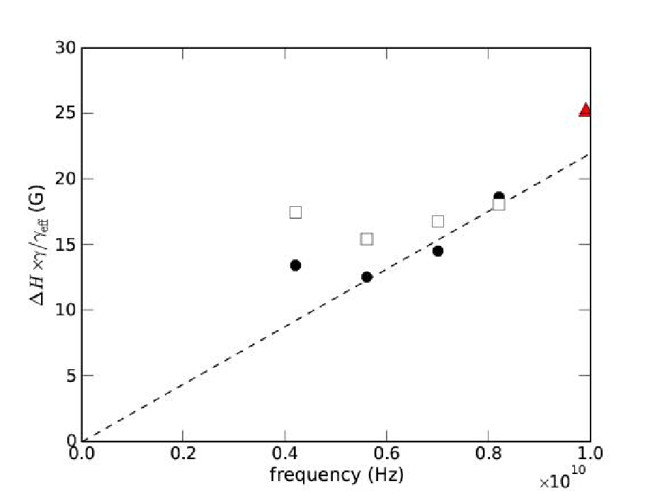
Another important characterization concerns the width of the resonance line. The full circles and open boxes in Fig.18 are the line widths measured as a function of frequency in the Py disks of diameters m and m, respectively. All values have been renormalized by the effective gyromagnetic ratio . These line widths are among the smallest reported for Py, confirming the excellent quality of the material used for this study.
The resonance line width (half-width at mid-height of the absorption curve) of the Py polycrystalline magnetic layer is described [36] as the sum of two contributions:
| (35) |
The first term relates to the intrinsic relaxation rate of the magnetization vector whereas the second term corresponds to the inhomogeneous broadening induced by a distribution of internal field, as well as by a distribution of polarization angles, of characteristics widths and , respectively. reflects the spatial inhomogeneity of the field parameter whereas refers to the distribution of the orientation of the applied field with respect to the normal to the surface of the individual crystallites.
The results obtained on the disks should be compared to the value observed by cavity-FMR on the extended thin film. In the cavity-FMR studies, the line widths measured on the film grown on the atomically flat Si substrate in the parallel and in the perpendicular geometries are equal (25 Oe) and reflect almost entirely the homogeneous contribution. The measured value is represented by a red triangle in Fig.18. It allows for an estimate of the intrinsic damping parameter (), found to be . This value is an upper bound for , since the presence of a small inhomogeneous contribution in the line width would reduce the value of the homogeneous part. The film grown on mica presents more inhomogeneities than on Si, the results of which corresponds to a line width increase of 3 Oe. This is due to the even surface of the mica substrate, which bends over because of the strain between the different sheets of mica.
From the frequency dependence of the line width of the large disk, we can estimate the damping coefficient in the nanostructure, found to be (dashed line on Fig.18), in good agreement with the upper bound found on the thin film. We find that there is no inhomogeneous broadening in the nanostructure, which means that the small amount observed in the extended film deposited on mica is not relevant in structures confined at the sub-micron length scale [13, 10]. It also implies that there is no additional broadening induced by the mechanical-FMR. Finally, the frequency dependence of the line width at low frequencies and of the small disk is not linear. In fact, the magnetization configuration becomes not uniform at low applied field, and the renormalization of the field line widths by is not sufficient to recover the intrinsic behavior. Moreover it was shown on the extended thin film that as the applied field is decreased, the increase of the angle between the equilibrium magnetization and the normal of the film increases the line width, through the inhomogeneous contribution associated [36] to the distribution in Eq.35.
VI Conclusion
It was shown in this article how MRFM can be used to detect and quantitatively analyze the intrinsic FMR spectra of individual sub-micron size samples. To realize this objective, the coupling between the magnetic probe attached to the cantilever and the sample has to be optimized. On one hand, it has to be as strong as possible to detect FMR in tiny samples. On the other hand, the inhomogeneity induced by the stray field of the probe has to be small compared to the internal dipolar field inhomogeneity in the sample, in order to detect the intrinsic behavior of the latter. Using a magnetic sphere whose size is of the order of the disk-shaped samples enables to meet these two requirements. We demonstrate a 1000 spins sensitivity at room temperature. Using two approximate 2D and 3D models, we can understand the measured FMR-spectra on Py disks patterned out from the same extended film, whose characteristics are well known. It requires a good understanding of finite size effects and of the homogeneous shift of the the SW modes resonance fields induced by the probe.
Finally, we would like to summarize the main advantages of mechanical-FMR: i) its sensitivity to detect a single magnon excitation in a buried hybrid structure, e.g. below contact electrodes, ii) its versatility as a near field technique (i.e. only sensitive to the area directly underneath the probe), which allows spatial imaging of the magnetization dynamics, and iii) its ability to measure the longitudinal component of the magnetization, a quantity directly linked to the damping.
We are greatly indebted to O. Acher and A.-L. Adenot for their help and support. This research was partially supported by the ANR PNANO06-0235 and by the European Grant NMP-FP7 212257-2 MASTER.
Appendix A Depolarization factors of a cylinder
The analytical formula that have been used for the demagnetization tensor, , of a disk of radius and thickness are explicitly written in this appendix. The formula are actually derived from the published work of S. Tandon [42] but we have chosen to reprint them below because a couple of small typos remain in the original paper. The only assumption made here is that the magnetization is homogeneous inside the cylindrical volume.
Because of the axial symmetry, the values of the tensor are better expressed in the cylindrical coordinates and, using the notation of Ref.[42], we introduce the reduced units :
| (1a) | ||||
| (1b) | ||||
| (1c) | ||||
where the notations and are respectively the distance (in reduced units) with the bottom and top surface of the cylinder. The function and design respectively the Sign and Heavisde functions:
The integrals have the following expressions:
| (2a) | ||||
| (2b) | ||||
| (2c) | ||||
where
| (3a) | |||||
| (3b) | |||||
and are the complete elliptic integrals of the first and second kind and is the Heuman’s Lambda function.
The above expressions are valid everywhere in space. The magnetic field induction at every point in space (inside or outside the sample’s volume) simply obeys the formula:
| (4) |
where is a function equals to 1 inside the cylindrical volume and 0 otherwise:
Appendix B Linearization in the local frame
The notations have been defined in Fig.11: is the Cartesian frame along the principal axis of the disk, with oriented along the normal and the Cartesian frame of the magnetization dynamics, with along the equilibrium (or effective magnetic field) direction. Both frames are related by a rotation of an angle around the direction. If is the angle that the external magnetic field makes with the normal of the disk, then is implicitly defined by the equilibrium condition:
| (5) |
In all the expressions above, the tensors are expressed in the Cartesian frame of the disk . This applies for the demagnetizing factors in appendix A, but also for the matrices:
| (6) |
| (7) |
Solving Eq.(24) requires to write down the different tensors in the local frame of the magnetization. This is achieved through the transformation , where is the rotation matrix between the and :
| (8) |
and the subscript stands for the transpose.
This allows us to find the expression Eqs.(29), where we have used symmetry arguments to impose .
References
- [1] H. Stoll, A. Puzic, B. van Waeyenberge, P. Fischer, J. Raabe, M. Buess, T. Haug, R. Höllinger, C. Back, D. Weiss, et al., Appl. Phys. Lett. 84, 3328 (2004).
- [2] Y. Acremann, J. P. Strachan, V. Chembrolu, S. D. Andrews, T. Tyliszczak, J. A. Katine, M. J. Carey, B. M. Clemens, H. C. Siegmann, and J. Stohr, Phys. Rev. Lett. 96, 217202 (2006).
- [3] J. Vogel, W. Kuch, M. Bonfim, J. Camarero, Y. Pennec, F. Offi, K. Fukumoto, J. Kirschner, A. Fontaine, and S. Pizzini, Appl. Phys. Lett. 82, 2299 (2003).
- [4] K. Perzlmaier, M. Buess, C. H. Back, V. E. Demidov, B. Hillebrands, and S. O. Demokritov, Phys. Rev. Lett. 94, 057202 (2005).
- [5] W. K. Hiebert, A. Stankiewicz, and M. R. Freeman, Phys. Rev. Lett. 79, 1134 (1997).
- [6] A. Barman, V. V. Kruglyak, R. J. Hicken, A. Kundrotaite, and M. Rahman, Appl. Phys. Lett. 82, 3065 (2003).
- [7] M. Buess, R. Höllinger, T. Haug, K. Perzlmaier, U. Krey, D. Pescia, M. R. Scheinfein, D. Weiss, and C. H. Back, Phys. Rev. Lett. 93, 077207 (2004).
- [8] A. A. Tulapurkar, Y. Suzuki, A. Fukushima, H. Kubota, H. Maehara, K. Tsunekawa, D. D. Djayaprawira, N. Watanabe, and S. Yuasa, Nature 438, 339 (2005).
- [9] J. C. Sankey, P. M. Braganca, A. G. F. Garcia, I. N. Krivorotov, R. A. Buhrman, and D. C. Ralph, Phys. Rev. Lett. 96, 227601 (2006).
- [10] W. Chen, J.-M. L. Beaujour, G. de Loubens, A. D. Kent, and J. Z. Sun, Appl. Phys. Lett. 92, 012507 (2008).
- [11] Z. Zhang, P. C. Hammel, and P. E. Wigen, Appl. Phys. Lett. 68, 2005 (1996).
- [12] V. Charbois, V. V. Naletov, J. B. Youssef, and O. Klein, Appl. Phys. Lett. 80, 4795 (2002).
- [13] G. de Loubens, V. V. Naletov, O. Klein, J. B. Youssef, F. Boust, and N. Vukadinovic, Phys. Rev. Lett. 98, 127601 (2007).
- [14] C. Herring and C. Kittel, Phys. Rev. 81, 869 (1951).
- [15] M. Bailleul, R. Hollinger, and C. Fermon, Phys. Rev. B 73, 104424 (2006).
- [16] P. E. Wigen, Thin Solid Films 114, 135 (1984).
- [17] O. Klein, S. Donovan, M. Dressel, and G. Grüner, Int. J. of Infrared and Millimeter Waves 14, 2423 (1993).
- [18] S. Donovan, O. Klein, M. Dressel, K. Holczer, and G. Grüner, Int. J. of Infrared and Millimeter Waves 14, 2459 (1993).
- [19] N. Bloembergen and S. Wang, Phys. Rev. 93, 72 (1954).
- [20] R. C. Fletcher, R. C. LeCraw, and E. G. Spencer, Phys. Rev. 117, 955 (1960).
- [21] H. Suhl, J. Phys. Chem. Solids 1, 209 (1957).
- [22] D. Rugar, R. Budakian, H. J. Mamin, and B. W. Chui, Nature 430, 329 (2004).
- [23] H. J. Mamin, M. Poggio, C. L. Degen, and D. Rugar, Nature Nanotechnology 2, 301 (2007).
- [24] O. Klein, V. Charbois, V. V. Naletov, and C. Fermon, Phys. Rev. B 67, 220407 (2003).
- [25] J. A. Sidles, J. L. Garbini, K. J. Bruland, D. Rugar, O. Züger, S. Hoen, and C. S. Yannoni, Rev. Mod. Phys. 67, 249 (1995).
- [26] Y. Obukhov, D. V. Pelekhov, J. Kim, P. Banerjee, I. Martin, E. Nazaretski, R. Movshovich, S. An, T. J. Gramila, S. Batra, et al., Phys. Rev. Lett. 100, 197601 (2008).
- [27] K. Holczer, O. Klein, and G. Grüner, Solid State Comm. 78, 875 (1991).
- [28] G. de Loubens, V. V. Naletov, and O. Klein, Phys. Rev. B 71, 180411 (2005).
- [29] H. J. Mamin and D. Rugar, Appl. Phys. Lett. 79, 3358 (2001).
- [30] O. Klein and V. V. Naletov, Comptes Rendus Physique 5, 325 (2004).
- [31] G. de Loubens, Ph.D. thesis, Université Paris XI - Orsay (2005), URL http://tel.archives-ouvertes.fr/tel-00118828/fr/.
- [32] R. Urban, A. Putilin, P. E. Wigen, S.-H. Liou, M. C. Cross, P. C. Hammel, and M. L. Roukes, Phys. Rev. B 73, 212410 (2006).
- [33] R. W. Damon and J. R. Eshbach, J. Phys. Chem. Solids 19, 308 (1961).
- [34] B. A. Kalinikos and A. N. Slavin, J. Phys. C: Solid State Phys. 19, 7013 (1986).
- [35] G. N. Kakazei, P. E. Wigen, K. Y. Guslienko, V. Novosad, A. N. Slavin, V. O. Golub, N. A. Lesnik, and Y. Otani, Appl. Phys. Lett. 85, 443 (2004).
- [36] H. Hurdequint, J. Magn. Magn. Mater. 242-245, 521 (2002).
- [37] H. Hurdequint, J. Magn. Magn. Mater. 310, 2061 (2007).
- [38] S. Mizukami, Y. Ando, and T. Miyazaki, J. Magn. Magn. Mater. 226, 1640 (2001).
- [39] S. Labbé and P.-Y. Bertin, J. Magn. Magn. Mater. 206, 93 (1999).
- [40] F. Boust and N. Vukadinovic, Phys. Rev. B 70, 172408 (2004).
- [41] K. Y. Guslienko, S. O. Demokritov, B. Hillebrands, and A. N. Slavin, Phys. Rev. B 66, 132402 (2002).
- [42] S. Tandon, M. Beleggia, Y. Zhu, and M. De Graef, J. Magn. Magn. Mater. 271, 9 (2004).